On non–Gaussianity in the Cosmic Microwave Background

Abstract

We consider a cosmological model with non–Gaussian initial perturbations, which in principle could be generated in non–standard inflationary scenarios with two or more scalar fields. In particular we focus our attention on the model proposed by Linde and Mukhanov (1997), where perturbations are quadratic in a Gaussian field. These perturbations, if they exist, have to be observable as a non-Gaussian distribution of the CMB signal on the sky. In order to efficiently pick up the non–Gaussian signal in CMB maps of degree resolution, one can use Minkowski Functionals and peak statistics. Our paper contains the theoretical predictions of the properties for Minkowski Functionals and distributions of peaks of the CMB anisotropy in the model with ”squared” Gaussian statistics. Likelihood comparison of the four–year COBE DMR data to this non–Gaussian model and the standard Gaussian model does not select any of them as most likely.

We also suggest an efficient algorithm for fast simulation of CMB maps on the whole sky. Using a cylindrical partition of the sphere, we rewrite the spherical harmonics analysis as a Fourier transform in flat space, which makes the problem accessible to numerically advantageous FFT methods.

1 Introduction

Observations of the Cosmic Microwave Background provide fundamental information about the primordial inhomogeneities in the Universe. The temperature anisotropies on scales above a few degrees preserve information about primordial density fluctuations on scales larger than the acoustic horizon at the moment of recombination. Since the first detection of the CMB anisotropy by the COBE satellite (Smoot et al. 1992; Bennett et al. 1996) several groups have also reported observations on angular scales of about $1\degr$ which roughly corresponds to the horizon size at recombination. Obtaining the spectrum of the primordial anisotropies on smaller scales with high precision will allow us to verify several robust predictions of inflation and permit to determine the values of important cosmological parameters with high accuracy. Future experiments (Bennett et al. 1995; Bersanelli et al. 1996) will yield all–sky maps of the CMB with sufficiently high resolution and sensitivity.

Apart from estimates of the power spectrum with subsequent parameter determination, the CMB data also provides very important constraints on the nature of the perturbations that led to the formation of large–scale structure (Bond and Jaffe 1998). To extract this information beyond the power spectrum we need to consider not only the amplitudes, but also the phases of the temperature field. One possible approach is under consideration in our paper.

Generally speaking, cosmological models based on the inflationary paradigm predict adiabatic Gaussian fluctuations with a power spectrum slightly different from the scale invariant one (Mukhanov and Chibisov 1981; see also Starobinsky 1982; Hawking 1982; Guth and Pi 1985; Bardeen et al. 1983). The Gaussianity of the density perturbations directly translates into Gaussianity of the CMB temperature fluctuations on the sky.

However, along with standard inflationary models, at present there still exist theories which are compatible with observations and predict non–Gaussian primordial fluctuations. Among them are, for instance, non–standard inflationary scenarios with two or more scalar fields, where one could expect significant deviations from Gaussianity (Linde and Mukhanov 1997; Antoniadis et al. 1997; Peebles 1999a, b), namely, the perturbations there are quadratic in a Gaussian field. Another possibility to accumulate non–Gaussianity in the CMB signals exists after recombination. Even if the fluctuations were Gaussian at the surface of the last scattering they may have acquired non–Gaussian contributions due to subsequent weak gravitational lensing (Fukushige et al. 1995; Bernardeau 1997) and due to various foregrounds like dust emission, synchrotron radiation, or unresolved point sources, to mention just a few (Banday et al. 1996). One should also take into account cosmic variance and additional non–Gaussian instrumental noise in the observational data (Tegmark 1997).

Therefore, establishing the Gaussian nature of the signal or detecting some distinctive non–Gaussianity is crucial. In fact, it would allow us to reveal the nature of the primordial fluctuations. For instance, a confirmation that the fluctuations of the CMB are Gaussian would leave practically no alternative to standard inflation, since it would definitely rule out most of the models that predict non–Gaussian fluctuations and are at present still compatible with observations. In addition, the investigation of non–Gaussianity is also important for a practical reason. Most of the current techniques for estimating the power spectrum from the observed signal with significant noise are optimised for the Gaussian fields only (Feldman et al. 1994; Knox et al. 1998; Ferreira et al. 1998).

Many authors have searched for non–Gaussian signatures in CMB data and in the large–scale structure using such diverse tests as peak statistics (Bardeen et al. 1986; Bond and Efstathiou 1987; Vittorio and Juskiewicz 1987), the genus curve (Coles 1988; Smoot et al. 1994), higher–order correlations (Luo and Schramm 1993), peak correlations (Kogut et al. 1996), and global Minkowski functionals (Gott III et al. 1990; Winitzki and Kosowsky 1997; Schmalzing and Górski 1998).

The first analysis of two–dimensional theoretical maps of the temperature fluctuations that used the total area, length of the boundary and genus for the excursion set was done by Gott III et al. (1990) although without referring to Minkowski functionals. Schmalzing and Górski (1998) discuss the application of the Minkowski functionals to all–sky maps taking into account the curvature of the celestial sphere. They apply these statistics to the high–latitude portion of the four–year COBE DMR data and argued for its advantage as a test of Gaussian signal. They conclude that the field is consistent with a Gaussian random field. Colley et al. (1996) measure the genus of the temperature fluctuations in the COBE DMR 4-year sky maps and come to a similar conclusion. Heavens (1999) compute the bispectrum of the four–year COBE datasets and again fail to find evidence for non–Gaussian behaviour.

However, Ferreira et al. (1998) study the distribution of an estimator for the normalised bispectrum and conclude that Gaussianity is ruled out at the confidence level at least of 99%. In a recent paper, Novikov et al. (1999) suggest to use the partial Minkowski functionals as quantitative descriptors of the geometrical properties of CMB maps. They apply their technique to the four–year DMR COBE data corrected for the Galaxy contamination and also find significant deviations from Gaussianity. It was later shown Banday et al. (2000) that the observed non–Gaussianity can be explained by systematics.

While these findings may appear confusing at first sight (Bromley and Tegmark 1999), they actually highlight the importance of studying non–Gaussian fields in a quantitative way. After all, while the Gaussian random field is a well–defined notion, non–Gaussian fields are still have to be substantiated. For instance, Kogut et al. (1996) introduce a non-Gaussian model where perturbations in $\ell$–space are drawn from independent $\chi_{\nu}^{2}$ distributions with $\nu$ degrees of freedom, while White (1999) puts forward the use of $\chi_{\nu}^{2}$ distributions in real rather than in $\ell$–space.

In our paper, we consider a cosmological model with non–Gaussian initial conditions, with a statistics in real space following a $\chi^{2}$ distribution with one degree of freedom. This type of perturbations results in very special non–Gaussianity of the CMB anisotropy. Therefore, it is well suited for the study of statistical methods. We calculate the Minkowski functionals and the distribution functions of extrema of the CMB field smoothed with COBE resolution in this model, and compare the outcome to the results for a Gaussian field with the same spectrum.

This article is organised as follows. In Section 2 we briefly review the definition of the Minkowski functionals and the distribution of extrema in two dimensions, and compare their expectation values for a Gaussian field and a $\chi^{2}$ field with the same smoothing scale and spectrum. As an aside, we investigate the behaviour of the one–point probability distribution under smoothing. In Section 3 we first outline an algorithm for doing Fast Fourier Transforms on the sphere that was used for our CMB map simulations. Afterwards, we compare the Minkowski functionals and the peak statistics of the COBE DMR data to both the Gaussian and the non–Gaussian model. Section 4 summarises and provides an outlook.

2 Theory

2.1 Gaussian and $\chi^{2}$ random fields

Let us consider the temperature fluctuations $\frac{\Delta{T}}{T}$ of the CMB temperature on the sky, parametrised with spherical coordinates $\vartheta$ and $\varphi$. Normalising with respect to the dispersion $\sqrt{\sigma}$, where $\sigma=\left\langle\left(\frac{\Delta{T}}{T}\right)^{2}\right\rangle$ is the variance of the temperature fluctuations, we obtain a random field $u(\vartheta,\varphi)$ with zero mean and unit variance: $\langle{u}\rangle=0$, $\langle{u^{2}}\rangle=1$.

In the following, we will consider two models for the random field given by the normalised temperature fluctuations on the sky.

The standard is to model $u$ as a Gaussian random field. The properties of Gaussian random fields are very well known (see e.g. Adler 1981).

Apart from that, we will also use a $\chi^{2}$ field with one degree of freedom, as suggested by the model of Linde and Mukhanov (1997). In order to retain zero mean and unit variance, we use the relation

$$\psi=\frac{1-\phi^{2}}{\sqrt{2}}$$ (1)

to calculate a realisation $\psi$ of a $\chi^{2}$ field from a given realisation $\phi$ of a Gaussian random field.

2.2 Minkowski functionals and peak statistics

Figure 1: The analytical expectation values of the Minkowski functionals for the Gaussian field (solid) and the $\chi^{2}$ field (dashed).

Figure 2: The analytical expectation values of the extrema distributions for the Gaussian field (solid) and the $\chi^{2}$ field (dashed).

Choosing a threshold $\nu$, we can divide the sphere into two parts: Hot regions where the random field $u$ passes the threshold, and cold regions where $u<\nu$. The hot region is also called the excursion set of the field $u$ over the threshold $\nu$. Its properties can be characterised by a large variety of geometrical quantities, including the Minkowski functionals (Minkowski 1903).

From the mathematical point of view, Minkowski functionals have several distinguishing properties. Hadwiger (1957) showed that all global morphological descriptors (satisfying translational invariance and additivity) for patterns in $d$-dimensional space are linear combinations of just $d+1$ Minkowski functionals $v_{\mu}(\nu)$, with $\mu\in\{0,\ldots,d\}$. Moreover, in up to four dimensions all Minkowski functionals have simple and intuitive geometrical meanings. In two dimensions these are:

Area:

$v_{0}(\nu)$ is the total area of all hot regions, that is points where $u(\vartheta,\varphi)>\nu$.

Boundary length:

$v_{1}(\nu)$ is proportional to the total length of the boundary between cold and hot regions.

Euler characteristic:

$v_{2}(\nu)$, being a purely topological quantity, counts the number of isolated hot regions minus the number of isolated cold regions. This is not exactly true on the sphere, where a generalised Gauss–Bonnet theorem holds (Allendoerfer and Weil 1943), but nevertheless we will use this relation in the following calculations.

Since Minkowski functionals are additive with respect to isolated parts of the sky, they can be used for patchy or incomplete coverage. Their calculation requires only $O(N)$ operations for calculating the Minkowski functionals on a map of $N$ pixels, once the first and second derivatives of the field at the pixel locations are known (Schmalzing and Górski 1998).

Both for a Gaussian and a $\chi^{2}$ random field, the Minkowski functionals in two dimensions are known analytically (Tomita 1990; Worsley 1994; Schmalzing 1999). Since the field is normalised to unit variance, the analytical values depend on a single parameter $\tau=\langle{u_{,i}^{2}}\rangle$, given as the variance of any of the field’s first derivatives. Note that $\tau$ has dimensions of inverse length squared, so one usually interprets $r_{\text{corr}}=(2\tau)^{-1/2}$ as the so–called “correlation length” of the random field $u$.

For the Gaussian random field, we have

$$\begin{split}v_{0}(\nu)&=\frac{1}{2}-\frac{1}{2}\Phi\left(\frac{\nu}{\sqrt{2}}\right),\\ v_{1}(\nu)&=\frac{\sqrt{\tau}}{8}\exp\left(-\frac{\nu^{2}}{2}\right),\\ v_{2}(\nu)&=\frac{\tau}{\sqrt{8\pi^{3}}}\nu\exp\left(-\frac{\nu^{2}}{2}\right).\end{split}$$ (2)

For the $\chi^{2}$ random field with one degree of freedom we have

$$\begin{split}v_{0}(\nu)&=\Phi\left(\sqrt{\frac{1}{2}-\frac{\nu}{\sqrt{2}}}\right),\\ v_{1}(\nu)&=\frac{\sqrt{\tau}}{4\sqrt{2}}\exp\left(-\frac{1}{2}+\frac{\nu}{\sqrt{2}}\right),\\ v_{2}(\nu)&=\frac{\tau}{4\pi\sqrt{\pi}}\sqrt{\frac{1}{2}-\frac{\nu}{\sqrt{2}}}\exp\left(-\frac{1}{2}+\frac{\nu}{\sqrt{2}}\right).\end{split}$$ (3)

Figure 1 shows a comparison of the expectation values of the Minkowski functionals of the Gaussian and $\chi^{2}$ random fields for the same parameter $\tau$.

By the Morse theorem (Morse and Cairns 1969), the Euler characteristic $\chi(\nu)$ of the excursion set above a certain threshold $\nu$ is related to the number of extrema above this threshold by

$$\chi(\nu)=N_{\text{max}}(\nu)+N_{\text{min}}(\nu)-N_{\text{sad}}(\nu).$$ (4)

Here $N_{\text{max}}(\nu)$, $N_{\text{min}}(\nu)$ and $N_{\text{sad}}(\nu)$ denote the number of maxima, minima and saddle points, respectively, where the value of the field itself lies above the threshold $\nu$. Along with the Minkowski functionals, we use these three distribution functions of all possible kinds of extrema – maxima, minima and saddle points – as another measure of non–Gaussianity. We always normalise these numbers by the total number $N_{\text{ext}}=N_{\text{max}}(-\infty)+N_{\text{min}}(-\infty)+N_{\text{sad}}(-\infty)$ of extrema in the field, giving number densities $n_{\text{max}}(\nu)$, $n_{\text{min}}(\nu)$ and $n_{\text{sad}}(\nu)$, respectively.

The peak statistics for the Gaussian random field have been thoroughly investigated (Bond and Efstathiou 1987; Bardeen et al. 1986), but unfortunately cannot be written in a simple form. The same holds for the $\chi^{2}$ field, whose extrema distribution functions are in principle easily obtained from the Gaussian case via Equation (1). Furthermore, the shapes of the Minkowski functional curves are universal, that is they do not depend on anything but the statistical nature (Gaussian or $\chi^{2}$) of the underlying random field, and the analytical expectation values only contain constants of proportionality, parametrised by the correlation radius $r_{\text{corr}}$. This is not the case for the distribution functions of extrema, where a second parameter $\gamma$ also affects the shape of the curves. We demonstrate this in Figure 2, by showing the expectation values for two different values of $\gamma$.

Since the Euler characteristic is proportional to the third Minkowski functional $v_{2}$, the distribution functions of extrema and the Minkowski functionals are not independent. In the following Section 3, we will use the first two Minkowski functionals $v_{0}$ and $v_{1}$, and the three distribution functions of extrema to test our models against the four–year COBE DMR data. However, let us first take a look at the effects of smoothing on non–Gaussian fields.

2.3 Non–Gaussianity and Gaussian smoothing

Figure 3: The PDFs of a smoothed $\chi^{2}$ random field (solid lines). From left to right, the smoothing scale increases, ranging from no smoothing (left panel) over little smoothing (middle panel) to considerable smoothing (right panel). The transition of the curve’s shape from clearly non–Gaussian to almost Gaussian is obvious. For comparison, the Gaussian bell curve is plotted in all three examples (dashed lines).

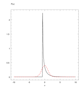
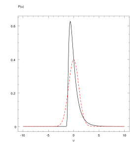
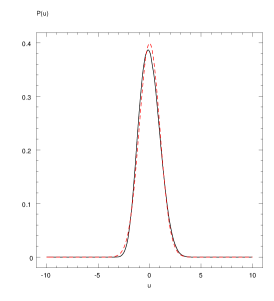
As an aside, we note that CMB temperature maps usually suffer from considerable smearing through the finite instrument beam size and are usually smoothed in order to reduce the noise level. Therefore, a non–Gaussian CMB signal may appear in the map with a much distorted distribution. Here, we attempt to quantify this effect. We focus on the one–point probability distribution (PDF) of the field, because it is easy to handle and also closely related to the zeroth Minkowski functional, being nothing but its nagative first derivative. It is of course conceivable that a non–Gaussian random field still has a Gaussian PDF. Other statistics can in principle be treated in a similar fashion.

We start from the cosmological CMB signal and consider it as a random field $u({\bf x})$ on some $d$–dimensional space, where in our case $d=2$. Introducing a smoothing filter $g({\bf x},t)$, where $t$ is the smoothing scale and $g({\bf x},0)=\delta({\bf x})$ – since the unsmoothed field should be equal to the original field – we obtain the smoothed field $u({\bf x},t)$ by convolution:

$$u({\bf x},t)={\mathcal{N}}(t)\int{\!{\rm d}^{d}y\,}g({\bf x}-{\bf y},t)u({\bf y}),$$ (5)

where the constant ${\mathcal{N}}(t)$ is chosen such that the smoothed field remains normalised to unit variance. We may think of $u({\bf x},t)$ as a field in $d+1$–dimensional “scale space” (ter Haar Romeny et al. 1991).

If the filter $g$ is Gaussian, it obeys the diffusion equation

$$\frac{\partial{g({\bf x},t)}}{\partial{t}}=t{\Delta}g({\bf x},t),$$ (6)

where the Laplacian $\Delta$ is of course taken with respect to the spatial coordinates ${\bf x}$ only.

Combining Equations (5) and (6), we can write down an “evolution equation” for the field $u$ as the scale $t$ changes:

$$\frac{\partial{u({\bf x},t)}}{\partial{t}}=t\left(\Delta+r_{\text{corr}}^{-2}\right)u({\bf x},t).$$ (7)

The second expression $r_{\text{corr}}^{-2}$ in the operator enters through the scale–dependence of the normalisation factor ${\mathcal{N}}(t)$. Details of the calculation can be found in Appendix A.

This equation enables us to study the one–point probability distribution $P(u,t)$ of the smoothed field $u(\cdot,t)$ as the smoothing scale changes. Writing this probability density as

$$P(u,t)=\left\langle\delta(u({\bf x},t)-u)\right\rangle$$ (8)

and applying the partial derivative with respect to $t$, we immediately obtain

$$\frac{\partial{P(u,t)}}{\partial{t}}=-t\frac{\partial}{\partial{u}}\left[\left(\langle\Delta{u}\rangle_{u}+\frac{u}{r_{\text{corr}}^{2}}\right)P(u,t)\right].$$ (9)

We refer the reader to Appendix B for the technical details of this calculation. The quantity $\langle\Delta{u}\rangle_{u}$ denotes the average of the Laplacian of the field $u({\bf x},t)$ under the condition that its value $u$ is fixed. It is interesting to note that this equation is written in conservative form, that is its integral over ${\!{\rm d}u\,}$ vanishes.

For a variety of random fields, the conditional average of the Laplacian can be calculated analytically. Most notably, for both the Gaussian and the $\chi^{2}$ field $\langle\Delta{u}\rangle_{u}=-\frac{u}{r_{\text{corr}}^{2}}$. In these cases, the right–hand side of Equation (9) simply becomes equal to zero.

As far as the Gaussian random field is concerned, $P(u)\propto\exp(-u^{2}/2)$ is a stationary solution of Equation (9). This reflects the well–known fact that a Gaussian random field stays Gaussian under smoothing, and in fact under any linear filtering.

In the case of the $\chi^{2}$ field, however, the probability distribution is non–zero only for $u<1/\sqrt{2}$ by Equation (1), and is not differentiable at the upper bound of the field. Therefore, under smoothing the field evolves away from the $\chi^{2}$ distribution, and finally ends up with a distribution close to the stationary Gaussian solution at large smoothing lengths. Figure 3 illustrates the effect using a $\chi^{2}$ random field with various degrees of smoothing.

This shows that although our two models are fairly different at first glance, the noise, beam size and other effects of actual observations tend to make the fields appear more similar. We shall look upon the practical consequences of this now, using the four–year COBE DMR data as an example.

3 Data analysis

Figure 4: Four maps showing realisations of the Gaussian and $\chi^{2}$ random fields and the northern and southern parts of the COBE DMR map, respectively. All maps extend from the pole to $30\degr$ latitude. The lines show isocontours of the field at half integer multiples of the standard deviation. Shaded areas indicate regions where the field value drops below the mean. Open circles show the positions of minima, full circles correspond to maxima, and saddle points are indicated by drude’s feet.

We illustrate our methods on the COBE DMR four–year all–sky maps (Bennett et al. 1996). We work with the map constructed from all three bands and both channels of the DMR instrument by the so–called subtraction method. Although this method is supposed to remove most of the galactic contamination, we avoid the galactic plane completely by applying a cut to $45\degr$ latitude.

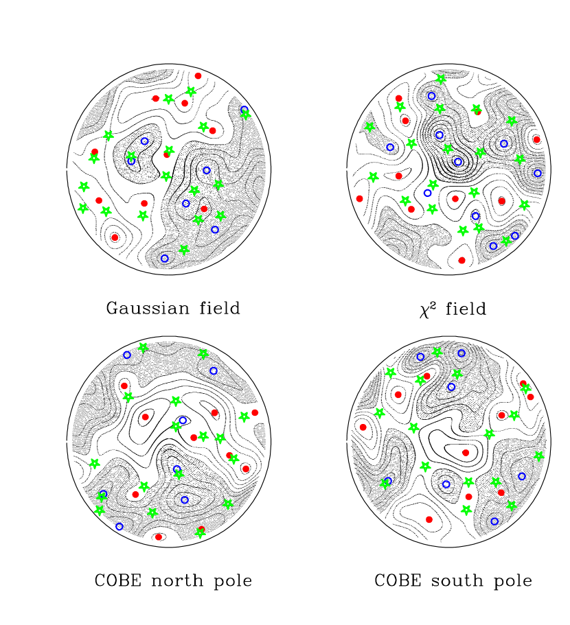
For the statistical tests presented in the following, we use a large number of realizations of the Gaussian and $\chi_{1}^{2}$ random fields. In both cases, we calculate the fields using a scale–free spectrum with a correlation radius of $1\degr$. To mimic the DMR beam, we smooth the fields with a Gaussian filter of $7\degr$ FWHM. Examples of realisations of the Gaussian and the $\chi^{2}$ random fields, together with the COBE DMR maps, are shown in Figure 4.

3.1 Fast Fourier Transform on the sphere

Figure 5: A COBE all–sky map, projected onto the plane in cylindrical coordinates and mirrored at the North pole to give a square suitable for the FFT method described in the text. The meaning of the various line and symbol styles is explained in the caption of Figure  4.

Statistical tests on CMB maps usually involve simulating large numbers of model maps from given power spectra. The naïve approach to this computational task is extremely time–consuming, requiring ${\mathcal{O}}(N^{2}M^{2})$ operations, where $N$ and $M$ are the number of pixels on the equator and the number of multipoles, respectively. Here we use a Fast Fourier Transform (FFT) in flat space over spherical coordinates outlined by Risbo (1996). This means that the FFT is used in both the polar and the azimuthal direction, while other methods usually perform the FFT over the polar angle alone. Let us first outline the mathematical and computational ideas.

Given a realisation of a random field in terms of its spherical harmonics coefficients $a_{{\ell}m}$, we wish to calculate its values $u(\vartheta,\varphi)$ in real space parametrised with spherical coordinates $(\vartheta,\varphi)$. This can be done through the spherical harmonics expansion

$$u(\vartheta,\varphi)=\sum_{\ell=0}^{M-1}\sum_{m=-\ell}^{+\ell}a_{{\ell}m}Y_{{\ell}m}(\vartheta,\varphi),$$ (10)

where the functions $Y_{{\ell}m}$ are the spherical harmonics. They are related to the associated Legendre functions $P_{{\ell}m}$ by

$$Y_{{\ell}m}(\vartheta,\varphi)=h_{{\ell}m}P_{{\ell}m}(\cos\vartheta){\rm e}^{im\varphi},$$ (11)

where $m$ and $\ell$ are called the order and the degree of the function, respectively, and

$$h_{{\ell}m}=\sqrt{\frac{2\ell+1}{4\pi}\frac{(\ell-m)!}{(\ell+m)!}}.$$ (12)

All spherical harmonics $Y_{{\ell}m}$ enjoy the symmetry property

$$Y_{{\ell}m}(\vartheta,\varphi)=Y_{{\ell}m}(2\pi-\vartheta,\pi+\varphi).$$ (13)

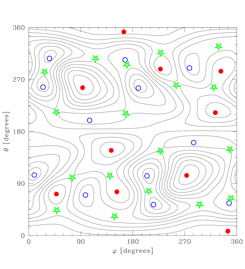
This can be used to extend the field $u(\vartheta,\varphi)$, which is normally defined for $(\vartheta,\varphi)\in[0,\pi]\times[0,2\pi]$, to the whole square $[0,2\pi]^{2}$, simply by mirroring the field at the point $(\pi,\pi)$. The resulting square map is illustrated by an example in Figure 5.

The extended field in real space, which now consists of two identical copies of the actual map, is periodic both in $\vartheta$ and in $\varphi$, and can therefore be expanded into a real–space Fourier series:

$$u(\vartheta,\varphi)=\sum_{j=0}^{M-1}\sum_{k=0}^{M-1}b_{jk}{\rm e}^{ij\vartheta+ik\varphi},$$ (14)

Inverting Equation (14) and inserting Equation (10) allows us to establish a relation between the Fourier coefficients and the spherical harmonics coefficients $a_{{\ell}m}$:

$$b_{jk}=\sum_{\ell=k}^{M-1}\left.a_{{\ell}m}h_{{\ell}m}p_{{\ell}mj}\right|_{m=k}\\ +\sum_{\ell=M-k}^{M-1}\left.a_{{\ell}m}h_{{\ell}m}p_{{\ell}mj}\right|_{m=k-M},$$ (15)

where the $p_{{\ell}mj}$ are the coefficients of the Fourier series of the associated Legendre functions:

$$P_{{\ell}m}(\cos\vartheta)=\sum_{j=0}^{M-1}{\rm e}^{ij\vartheta}p_{{\ell}mj}.$$ (16)

Using the well–known (Press et al. 1987) recurrence relation for the associated Legendre functions, it is easy to derive recurrence relations for numerical evaluation of the $p_{{\ell}mj}$.

Let us now summarise the steps for efficiently calculating a CMB map in real space from its spherical harmonics coefficients.

1. Obtain a realisation of the random field in spherical harmonics $a_{{\ell}m}$.

2. Calculate the intermediate Fourier coefficients $b_{jk}$ using Equation (15). This step requires ${\mathcal{O}}(M^{3})$ operations.

3. Perform the two–dimensional Fast Fourier Transform from Equation (14) in order to obtain the real–space realisation $u(\vartheta,\varphi)$. This step requires ${\mathcal{O}}(N^{2}\log{M})$ operations.

Obviously, our approach produces a cylindrical pixelisation in real space, resulting in non–uniform pixels. This makes it unsuitable for applications that involve quadratures, where uniform pixelisations (e.g. Gorski et al. 1999) are desirable. However, the method is well suited for the calculations presented below, because it allows large oversampling of the map in real space, that is $N\ll{M}$, with little computational effort. This is desirable both for accurate calculations of Minkowski functionals of a map by tracing the contours with high accuracy, and for determining the exact positions of extrema.

3.2 Minkowski functionals

		$P_{\text{area}}$	$P_{\text{length}}$	$P_{\text{max}}$	$P_{\text{min}}$	$P_{\text{sad}}$
South	Gaussian	94%	12%	38%	52%	53%
	$\chi_{1}^{2}$	87%	61%	44%	56%	57%
North	Gaussian	33%	44%	89%	87%	95%
	$\chi_{1}^{2}$	31%	28%	76%	81%	88%

Table 1: Summary of the probabilities of obtaining the COBE DMR data as a realisation of the models – a Gaussian random field and a $\chi^{2}$ random field – considered here. The analysis is done separately for the Northern and Southern polar caps. Since we use five related statistics to obtain these probabilities, five values are shown for each case.

Figure 6: The Minkowski functionals of the COBE DMR data in comparison with the average values for a Gaussian random field. The areas indicate the standard deviation.

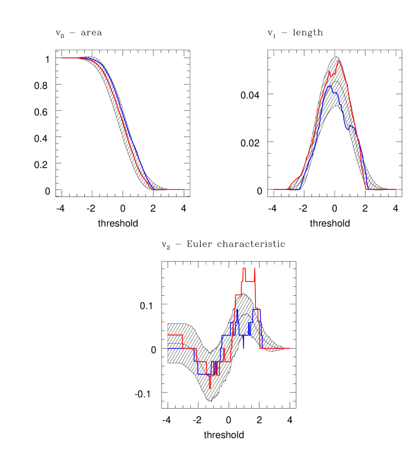
The Minkowski functionals of the COBE DMR maps are displayed in Figure 6. Since the Northern and Southern polar caps were analysed separately, we show two curves in each panel. The shaded areas indicate the average and standard deviation of 1000 realisations of a Gaussian random field with the same two–point characteristics as the COBE data.

In order to assess the probability that the COBE DMR maps are indeed a realisation of our toy models, we use a non–parametric test (Novikov et al. 2000).

We computed $N=1000$ realisation of each random field. The $n$th realisation yields Minkowski functionals $V_{\mu}^{(n)}(\nu)$, with the threshold $\nu$ ranging from $-5$ to $5$. We calculate the average Minkowski functionals

$${\overline{V}}_{\mu}(\nu)=\frac{1}{N}\sum_{n=1}^{N}V_{\mu}^{(n)}(\nu)$$ (17)

for the random field, and determine the $L_{1}$–distance of each realisation from this average:

$$\Delta_{\mu}^{(n)}=\int{\rm d}\nu\left|V_{\mu}^{(n)}(\nu)-{\overline{V}}_{\mu}(\nu)\right|.$$ (18)

We then obtain the same quantity $\Delta_{\mu}^{\text{COBE}}$ from the data, and test the hypothesis that this $\Delta_{\mu}^{\text{COBE}}$ is distributed according to the distribution function of the $\Delta_{\mu}^{(n)}$ of the model we are currently investigating.

The resulting probabilities are displayed in Table 1. Note that we only show the values for the first two functionals, the area $V_{0}$ and the length $V_{1}$, since by Equation (4) the last Minkowski functional is a linear combination of the extrema statistics analysed in Section 3.3.

3.3 Distribution of extrema

Figure 7: The extrema statistics of the COBE DMR data in comparison with the average values for a Gaussian random field. The areas indicate the standard deviation.

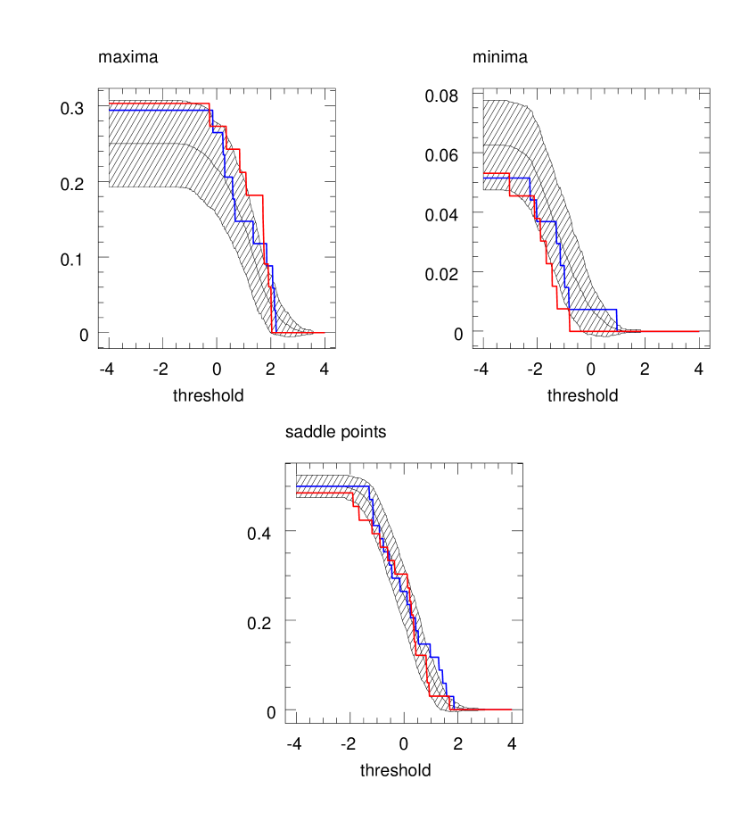
For the COBE DMR data, the distribution functions of all three kinds of extrema are shown in Figure 7. For comparison, we also show the mean and standard deviations over 1000 realisations of a Gaussian random field with the same two–point characteristics.

In order to quantify the difference of the COBE data and the models, we use a standard Kolmogorov–Smirnov test (Press et al. 1987). The resulting probabilities are shown in Table 1.

4 Summary and Outlook

We have investigated a method for probing the non–Gaussianity of CMB maps, based on Minkowski functionals and on distribution functions of extrema. In order to make the deviations from Gaussianity quantitative, we used a model proposed by Linde and Mukhanov (1997), producing to a $\chi^{2}$ distribution with one degree of freedom for the primordial fluctuations. Analytical calculations for our statistics showed that the non–Gaussian and Gaussian models produce markedly different results.

The situation may change, however, when smoothing is taken into account. We derived an equation governing the change of the one–point probability distribution with the smoothing scale and found that, while the Gaussian field remains Gaussian under smoothing, the $\chi^{2}$ field evolves towards a more symmetric distribution with closer resemblance to the Gaussian bell. The outcome of this effect became clear in an application of the method to the COBE DMR data – we saw a slight preference of the Gaussian model, but this was by no means significant. Since all realisations of the maps were highly oversampled in real space, the failure to discriminate between the two models is definitely due to the rather large smoothing scale. Therefore, an application of the method to the recently completed Boomerang (de Bernadis et al. 2000) and MAXIMA (Hanany et al. 2000) experiments appears highly promising, as soon as the data become available.

Appendix A Derivation of Equation (7)

We start from the smoothing prescription in Equation (5):

$$u({\bf x},t)={\mathcal{N}}(t)\int{\!{\rm d}^{d}y\,}g({\bf x}-{\bf y},t)u({\bf y}),$$ (19)

and apply the partial derivative with respect to the smoothing scale $t$. Straightforward differentiation yields

$$\frac{\partial{u({\bf x},t)}}{\partial{t}}=\\ \frac{\partial{{\mathcal{N}}(t)}}{\partial{t}}\int{\!{\rm d}^{d}y\,}g({\bf x}-{\bf y},t)u({\bf y})+\\ {\mathcal{N}}(t)\int{\!{\rm d}^{d}y\,}\frac{\partial{g({\bf x}-{\bf y},t)}}{\partial{t}}u({\bf y}).$$ (20)

We use the diffusion equation (6) on the second addend, and eliminate the integrals by reinserting the smoothing prescription (5). This leads to:

$$\frac{\partial{u({\bf x},t)}}{\partial{t}}=\frac{\frac{\partial{{\mathcal{N}}(t)}}{\partial{t}}}{{\mathcal{N}}(t)}u({\bf x},t)+t{\Delta}u({\bf x},t).$$ (21)

In order to evaluate the partial derivative of the normalisation factor ${\mathcal{N}}(t)$, we use the normalisation condition

$$1=\int{\!{\rm d}^{d}x\,}u({\bf x},t)^{2}$$ (22)

and again apply the partial derivative with respect to $t$. Together with Equation (21), this becomes

$$\begin{split}0&=\int{\!{\rm d}^{d}x\,}u({\bf x},t)\frac{\partial{u({\bf x},t)}}{\partial{t}}\\ &=\frac{\frac{\partial{{\mathcal{N}}(t)}}{\partial{t}}}{{\mathcal{N}}(t)}\int{\!{\rm d}^{d}x\,}u({\bf x},t)^{2}+t\int{\!{\rm d}^{d}x\,}u({\bf x},t){\Delta}u({\bf x},t)\\ &=\frac{\frac{\partial{{\mathcal{N}}(t)}}{\partial{t}}}{{\mathcal{N}}(t)}-t\times r_{\text{corr}}^{-2}.\end{split}$$ (23)

The first integral is equal to one because of the normalisation condition (22), while the second integral can be rewritten as the variance of the gradient of $u({\bf x},t)$ using partial integration, which is equal to the inverse square of the correlation radius $r_{\text{corr}}$ by definition.

Now we can eliminate the explicit reference to the normalisation factor ${\mathcal{N}}(t)$ from Equation (21) and obtain our final result, Equation (7):

$$\frac{\partial{u({\bf x},t)}}{\partial{t}}=t\left(\Delta+r_{\text{corr}}^{-2}\right)u({\bf x},t).$$ (24)

Appendix B Derivation of Equation (9)

This time, we investigate the properties of the one–point probability distribution function $P(u)$ under smoothing. We start from the definition (8):

$$P(u,t)=\left\langle\delta(u({\bf x},t)-u)\right\rangle.$$ (25)

It is a common bad habit among physicists to use the same notation for utterly different things. We are no expection to this, employing the same letter both for the smoothed random field and for the argument of the probability distribution. However, we always add the scale space coordinate $({\bf x},t)$ to the random field $u({\bf x},t)$ , while the value $u$ has no such argument.

At first, the partial derivative of this equation yields a functional derivative of the $\delta$–function with respect to the field $u({\bf x},t)$. Fortunately, it can be rewritten as an ordinary partial derivative with respect to the value $u$. Furthermore, the value $u$ (not the field $u({\bf x},t)$!) only enters through the $\delta$–function. We can then insert Equation (7) for the evolution of the field under smoothing. All in all, the calculation proceeds as follows:

$$\begin{split}\frac{\partial{P(u,t)}}{\partial{t}}&=\left\langle\frac{\partial{\delta(u({\bf x},t)-u)}}{\partial{u({\bf x},t)}}\times\frac{\partial{u({\bf x},t)}}{\partial{t}}\right\rangle\\ &=-\frac{\partial}{\partial{u}}\left\langle\delta(u({\bf x},t)-u)\frac{\partial{u({\bf x},t)}}{\partial{t}}\right\rangle\\ &=-t\frac{\partial}{\partial{u}}\left\langle\delta(u({\bf x},t)-u)\left(\Delta+r_{\text{corr}}^{-2}\right)u({\bf x},t)\right\rangle\\ &=-t\frac{\partial}{\partial{u}}\left\langle\delta(u({\bf x},t)-u)\left({\Delta}u({\bf x},t)+\frac{u}{r_{\text{corr}}^{2}}\right)\right\rangle\\ &=-t\frac{\partial}{\partial{u}}\left[\left(\langle\Delta{u}\rangle_{u}+\frac{u}{r_{\text{corr}}^{2}}\right)P(u,t)\right],\end{split}$$ (26)

so we end up with Equation (9).

References

- Gott III et al. (1990) Gott III, J. R., Park, C., Juszkiewicz, R., Bies, W. E., Bennett, D. P., Bouchet, F. R., and Stebbins, A., 1990, ApJ 352, 1
- Smoot et al. (1992) Smoot, G. F., Bennett, C. L., Kogut, A., Wright, E. L., Aymon, J., Boggess, N. W., Cheng, E. S., De Amici, G.and Gulkis, S., Hauser, M. G., Hinshaw, G., Jackson, P. D., Janssen, M., Kaita, E., Kelsall, T., Keegstra, P., Lineweaver, C., Loewenstein, K., Lubin, P., Mather, J., Meyer, S. S., Moseley, S. H., Murdock, T., Rokke, L., Silverberg, R. F., Tenorio, L., Weiss, R., and Wilkinson, D. T., 1992, ApJ 396, L1
- Adler (1981) Adler, R. J., 1981, The geometry of random fields, John Wiley & Sons, Chichester
- Allendoerfer and Weil (1943) Allendoerfer, C. B. and Weil, A., 1943, Trans. Amer. Math. Soc. 53, 101
- Antoniadis et al. (1997) Antoniadis, I., Mazur, P. O., and Mottola, E., 1997, Comment on ”Nongaussian Isocurvature Perturbations from Inflation”, astro-ph/9705200
- Banday et al. (1996) Banday, A. J., Górski, K. M., Bennett, C. L., Hinshaw, G., Kogut, A., and Smoot, G. F., 1996, ApJ 468, L85
- Banday et al. (2000) Banday, A. J., Zaroubi, S., and Górski, K. M., 2000, ApJ 533, 575
- Bardeen et al. (1986) Bardeen, J. M., Bond, J. R., Kaiser, N., and Szalay, A. S., 1986, ApJ 304, 15
- Bardeen et al. (1983) Bardeen, J. M., Steinhardt, P. J., and Turner, M. S., 1983, Phys. Rev. D 28, 679
- Bennett et al. (1996) Bennett, C. L., Banday, A., Górski, K. M., Jackson, P. D., Keegstra, P. B., Kogut, A., Smoot, G. F., Wilkinson, D. T., and Wright, E. L., 1996, ApJ 464, L1
- Bennett et al. (1995) Bennett, C. L., Hinshaw, G., Jarosik, N. C., Mather, J., Meyer, S. S., Page, L., Skillman, D., Spergel, D. N., Wilkinson, D. T., and Wright, E. L., 1995, BAAS 187(71.09), 1385
- Bernardeau (1997) Bernardeau, F., 1997, Astron. Astrophys. 324, 15
- Bersanelli et al. (1996) Bersanelli, M., Bouchet, F. R., Efstathiou, G., Griffin, M., Lamarre, J. M., Mandolesi, N., Norgaard-Nielsen, H. U., Pace, O., Polny, J., Puget, J. L., Tauber, J., Vittorio, N., and Volonté, S., 1996, COBRAS/SAMBA. A mission dedicated to imaging the anisotropies of the cosmic microwave background. Report on the phase A study, European Space Agency
- Bond and Efstathiou (1987) Bond, J. R. and Efstathiou, G., 1987, MNRAS 226, 655
- Bond and Jaffe (1998) Bond, J. R. and Jaffe, A. H., 1998, in Discussion Meeting on Large Scale Structure in the Universe, Royal Society, London
- Bromley and Tegmark (1999) Bromley, B. C. and Tegmark, M., 1999, Is the cosmic microwave background really non–Gaussian?, ApJ in press, astro-ph/9904254
- Coles (1988) Coles, P., 1988, MNRAS 234, 509
- Colley et al. (1996) Colley, W. N., Gott III, J. R., and Park, C., 1996, MNRAS 281, L82
- de Bernadis et al. (2000) de Bernadis, P., Ade, P. A. R., Bock, J. J., Bond, J. R., Borrill, J., Boscaleri, A., Coble, K., Crill, B. P., Gasperis, G. D., Farese, P. C., Ferreira, P. G., Ganga, K., Giacometti, M., Hivon, E., Hristov, V. V., Iacoangeli, A., Jaffe, A. H., Lange, A. E., Martinis, L., Masi, S., Mason, P. V., Mauskopf, P. D., Melchiorri, A., Miglio, L., Montroy, T., Netterfield, C. B., Pascale, E., Piacentini, F., Pogosyan, D., Prunet, S., Rao, S., Romeo, G., Ruhl, J. E., Scaramuzzi, F., Sforna, D., and Vittorio, N., 2000, Nature 404, 955
- Feldman et al. (1994) Feldman, H. A., Kaiser, N., and Peacock, J. A., 1994, ApJ 426, 23
- Ferreira et al. (1998) Ferreira, P. G., Magueijo, J. C. R., and Górski, K. M., 1998, ApJ 503, L1
- Fukushige et al. (1995) Fukushige, T., Makino, J., Nishimura, O., and Ebisuzaki, T., 1995, PASJ 47, 493
-
Gorski et al. (1999)
Gorski, K. M., Wandelt, B. D., Hansen, F. K., Hivon, E., and Banday, A. J.,
1999,
The HEALPix Primer,
Technical report, Theoretical Astrophysics Center (TAC) Kopenhagen,
http://www.tac.dk/~healpix/ - Guth and Pi (1985) Guth, A. H. and Pi, S.-Y., 1985, Phys. Rev. Lett. 49, 1110
- Hadwiger (1957) Hadwiger, H., 1957, Vorlesungen über Inhalt, Oberfläche und Isoperimetrie, Springer Verlag, Berlin
- Hanany et al. (2000) Hanany, S., Ade, P., Balbi, A., Bock, J., Borrill, J., Boscaleri, A., de Bernardis, P., Ferreira, P. G., Hristov, V. V., Jaffe, A. H., Lange, A. E., Lee, A. T., Mauskopf, P. D., Netterfield, C. B., Oh, S., Pascale, E., Rabii, B., Richards, P. L., Smoot, G. F., Stompor, R., Winant, C. D., and Wu, J. H. P., 2000, MAXIMA-1: A Measurement of the Cosmic Microwave Background Anisotropy on angular scales of 10 arcminutes to 5 degrees, submitted to ApJ, astro-ph/0005123
- Hawking (1982) Hawking, S. W., 1982, Phys. Lett. B 115, 295
- Heavens (1999) Heavens, A. F., 1999, MNRAS 299, 805
- Knox et al. (1998) Knox, L., Bond, J. R., Jaffe, A. H., Segal, M., and Charbonneau, D., 1998, Phys. Rev. D 58, 083004
- Kogut et al. (1996) Kogut, A., Banday, A. J., Bennett, C. L., Górski, K. M., Hinshaw, G., Smoot, G. F., and Wright, E. L., 1996, ApJ 464, L29
- Linde and Mukhanov (1997) Linde, A. and Mukhanov, V. F., 1997, Phys. Rev. D 56, 535
- Luo and Schramm (1993) Luo, X. and Schramm, D. N., 1993, ApJ 408, 33
- Minkowski (1903) Minkowski, H., 1903, Mathematische Annalen 57, 447, in German
- Morse and Cairns (1969) Morse, M. and Cairns, S. S., 1969, Critical point theory in global analysis and differential topology, Academic Press, New York and London
- Mukhanov and Chibisov (1981) Mukhanov, V. F. and Chibisov, G., 1981, JETP Letters 33, 532
- Novikov et al. (1999) Novikov, D. I., Feldman, H. A., and Shandarin, S. F., 1999, Int. J. Mod. Phys. D8, 291
- Novikov et al. (2000) Novikov, D. I., Naselsky, P., Jørgensen, H., Christensen, P., Novikov, I., and Nørgaard-Nielsen, H., 2000, Power filtration of CMB observational data, submitted, astro-ph/0001432
- Peebles (1999a) Peebles, P. J. E., 1999a, ApJ 510, 531
- Peebles (1999b) Peebles, P. J. E., 1999b, ApJ 510, 523
- Press et al. (1987) Press, W. H., Flannery, B. P., Teukolsky, S. A., and Vetterling, W. T., 1987, Numerical recipes in C, Cambridge University Press, Cambridge
- Risbo (1996) Risbo, T., 1996, Journal of Geodesy 70, 383
- Schmalzing (1999) Schmalzing, J., 1999, Ph.D. thesis, Ludwig–Maxmilians–Universität München
- Schmalzing and Górski (1998) Schmalzing, J. and Górski, K. M., 1998, MNRAS 297, 355
- Smoot et al. (1994) Smoot, G. F., Tenorio, L., J., B. A., Kogut, A., Wright, E. L., Hinshaw, G., and Bennett, C. L., 1994, ApJ 437, 1
- Starobinsky (1982) Starobinsky, A. A., 1982, Phys. Lett. B 117, 175
- Tegmark (1997) Tegmark, M., 1997, ApJ 480, L87
- ter Haar Romeny et al. (1991) ter Haar Romeny, B. M., Florack, L. M. J., Koenderink, J. J., and Viergever, M. A., 1991, in Lecture Notes in Computer Science, Vol. 511, pp 239–255, Springer Verlag, Berlin
- Tomita (1990) Tomita, H., 1990, in K. Kawasaki, M. Suzuki, and A. Onuki (eds.), Formation, dynamics and statistics of patterns, Vol. 1, pp 113–157, World Scientific
- Vittorio and Juskiewicz (1987) Vittorio, N. and Juskiewicz, R., 1987, ApJ 314, L29
- White (1999) White, M., 1999, Higher order moments of the density field in a parametrized sequence of non–Gaussian theories, to appear, astro-ph/9811227
- Winitzki and Kosowsky (1997) Winitzki, S. and Kosowsky, A., 1997, New Astronomy 3, 75
- Worsley (1994) Worsley, K., 1994, Adv. Appl. Prob. 26, 13