ITERATIVE MAP-MAKING FOR SCANNING EXPERIMENTS
We describe here an iterative method for jointly estimating the noise power spectrum from a scanning experiment’s time-ordered data, together with the maximum-likelihood map. We test the robustness of this method on simulated datasets with colored noise, like those of bolometer receivers in CMB experiments.
1 Introduction
The map-making problem for CMB anisotropy measurements was first considered in the context of the COBE-DMR mission . It was further extended to quick algorithms for differential measurements taking into account noise . Given the size of the upcoming datasets ( pixels for MAP) it is essential that the map-making algorithm remains quick (typically where is the number of time-samples, and the effective noise-filter length). Another related question, which has been pioneered by , is how to determine the noise statistical properties from the data itself. We present a map-making method based on Wright’s fast algorithm to compute iteratively a minimum variance map together with an estimate of the detector noise power spectrum which is needed to compute unbiased power spectrum estimators of the cosmological signal.
2 Iterative mapmaking - Application to simulations
2.1 Method
Following Tegmark , we model the data stream in the following way:
| (1) |
where is a pixelized version of the observed sky (i.e. convolved by the experimental beam), and is the detector noise after primary deconvolution of any filter present in the instrumental chain (e.g. bolometer time constant, read-out filters). We will assume here that the experiment is a total power measurement, i.e. that the pointing matrix contains only one non-zero element per row. We now want to estimate the minimum variance map from this data, ie the map that minimizes . The solution is given by:
| (2) |
A few remarks are necessary at this point. First, the matrix to be inverted
is huge () so that an iterative linear solver is needed.
Secondly, the noise correlation matrix has to be determined from
the data itself. To make this tractable we assume that, at least over subsets of
the time-stream, the noise is reasonably stationary, so that the multiplication by
becomes a convolution operator, in other words that it is diagonal
in Fourier space aaaThis is actually only approximately true since a convolution
operator is a circulant matrix, ie it assumes that the time-stream has periodic boundary
conditions; this is however a rather good approximation for a time-stream much longer
than the effective length of the noise-filter .
We thus implemented the following algorithm:
for each stationary noise subset • • endfor
To keep the algorithm as fast as possible, we took to be diagonal and constant, so that is diagonal, with each element beeing equal to the number of observations per pixel, up to a multiplicative constant. The choice of the numerical value of this constant is only important for the convergence properties of the algorithm. In this form, the algorithm is very similar to a Jacobi iterative solver (in which we would have instead of ). It has the additional advantage of being very easy to compute, for very similar convergence properties. Since we made the assumption that each noise matrix is diagonal in Fourier space, all time-domain operations are done in Fourier space using FFTs, thus reducing the number of floating point operations to for each subset.
The advantages of this iterative method are obvious: it is fast ( operations) and cheap in memory ( storage). However, since we try to estimate both the noise power spectrum and the map in a leap-frog manner, the convergence properties must be studied by means of numerical simulations.
2.2 Simulations
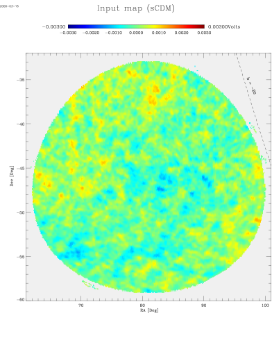
To test the convergence properties of the algorithm, we simulated a scanning experiment on a fake sCDM map with a gaussian beam of arcmin FWHM, and noise whose power spectrum is . To simulate the contamination of low frequencies by possible scan-synchronous systematics, we high-pass filtered the generated time-stream with a step filter. This has the effect of formally replacing the pointing matrix by where is the step filter; however, looking at Eq. 2, this is completely equivalent to leaving unchanged, and replacing by , which is straightforward in Fourier space.
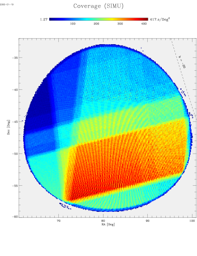
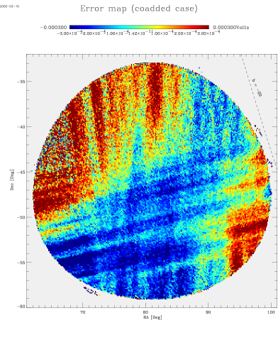
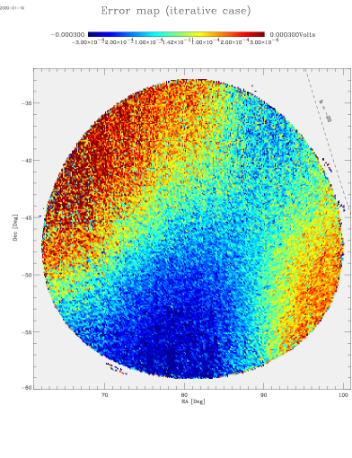
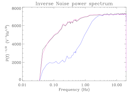
To be more specific, we used a spherical cap of HEALPix pixels of size generated from an sCDM COBE-normalized power spectrum, to generate a sample time stream. The sampling rate used is Hz, and the scan velocity deg/s. The sky coverage of the simulation is shown in Fig. . The same figure shows the input map used for the simulation, as well as the error map from the naive (coadded) map-making and the iterative map-making after iterations. One can see from those that the striping is much reduced in the iterative case, the only remaining feature in the error map being a large-scale mode that was lost in the high-pass filtering of the time-stream. Fig. shows the (inverse) noise power spectrum estimate compared to the data power spectrum and the true power spectrum. We can see that the estimated PS is very close to the input one.
As in any iterative linear solver, the convergence of the solution, decomposed on the (noise-) matrix eigenmodes, is a function of the associated eigenvalue. Thus the noisiest pixel modes (usually at large scales since the time-stream is high-pass filtered, either by hand or as part of the algorithm if the noise is higher at low frequency) take (exponantially) more time to converge. The problem scales as the noise matrix condition number, which is a direct function of the noise power spectrum dynamical range and of the scanning strategy. We propose to accelerate the convergence of the algorithm with the implementation of a multi-grid like method where the time-stream, as well as the pixels, get rebinned. This method will be described in a future paper.
3 Conclusions - Perspectives
We described a fast iterative map-making method to simultaneously generate the maximum-likelihood map and the noise power spectrum from a scanning experiment time stream. We tested its convergence properties on simulations, and concluded that, except for the spatially largest (and ill conditioned) modes, the map and noise power spectra converge very quickly. We propose to cure the convergence of this large scale modes by applying a multi-grid method to be described in a future publication.
References
References
- [1] P.G. Ferreira & A.H. Jaffe, MNRAS 312, 89 (2000)
- [2] K.M. Górski, E. Hivon, B.D. Wandelt in proceedings of the MPA/ESO Conference, Garching, 2-7 August 1998, eds A.J. Banday, R.K. Sheth and L. Da Costa. See also http://www.tac.dk/ healpix/
- [3] C.H. Lineweaver et al, Astrophys. Journal 436, 452 (1994)
- [4] M. Tegmark, Astrophys. Journal Lett. 480, 87 (1997)
- [5] E.L. Wright, in proceedings of the BCSPIN Puri Winter School
- [6] E.L. Wright, G. Hinshaw, C.L. Bennett, Astrophys. Journal Lett. 458, 53 (1996)
- [7] E.L. Wright, proceeding of the IAS CMB Workshop, astro-ph/9612006