HIIphot: AUTOMATED PHOTOMETRY OF H II REGIONS
APPLIED TO M51

Abstract

We have developed a robust, automated method, hereafter designated HIIphot, which enables accurate photometric characterization of H II regions while permitting genuine adaptivity to irregular source morphology. HIIphot utilizes object-recognition techniques to make a first guess at the shapes of all sources, then allows for departure from such idealized “seeds” through an iterative growing procedure. Photometric corrections for spatially coincident diffuse emission are derived from a low-order surface fit to the background after exclusion of all detected sources. We present results for the well-studied, nearby spiral M51 in which 1229 H II regions are detected above the $5\sigma$ level. A simple, weighted power-law fit to the measured H$\alpha$ luminosity function (H II LF) above log L${}_{H\alpha}=37.6$ gives $\alpha=-1.75\pm 0.06$, despite a conspicuous break in the H II LF observed near L${}_{H\alpha}=10^{38.9}$. Our best-fit slope is marginally steeper than measured by Rand (1992), perhaps reflecting our increased sensitivity at low luminosities and to notably diffuse objects. H II regions located in interarm gaps are preferentially less luminous than counterparts which constitute M51’s grand-design spiral arms and are best fit with a power-law slope of $\alpha=-1.96\pm 0.15$. We assign arm/interarm status for H II regions based upon the varying surface brightness of diffuse emission as a function of position throughout the image. Using our measurement of the integrated flux contributed by resolved H II regions in M51, we estimate the diffuse fraction to be approximately 0.45 – in agreement with the determination of Greenawalt et al. (1998). Automated processing of degraded narrowband datasets is undertaken in order to gauge (distance-related) systematic effects associated with limiting spatial resolution and sensitivity.

1 Introduction

H II regions are an effective optical tracer of ongoing massive star formation. Even a single early-type star produces enough Lyman continuum photons to ionize a quantity of gas sufficient to produce readily detectable recombination lines in galaxies at distances of many Mpc. Observations in the Balmer lines (predominantly H$\alpha$) and other nebular emission lines (e.g. [N II] $\lambda\lambda$ 6548,6584, [S II] $\lambda\lambda$ 6717,6731, and [O III] $\lambda$ 5007) enable estimation of physical conditions within discrete H II regions (Evans & Dopita (1985), Osterbrock (1989) ($AGN^{2}$), Ferland, et al. (1998)). Conversely, measurement of the H II region luminosity function can indicate global patterns in the process of star cluster formation (Kennicutt, Edgar & Hodge (1989) (hereafter KEH89), Banfi, Rampazzo, Chincarini & Henry (1993), Feinstein (1997), Wyder, Hodge & Skelton (1997)). An excellent review of the field is provided by Oey & Clarke (1998).

We sought a fully-automated technique for determination of the positions, fluxes, and sizes of H II regions in galaxies. Such a tool is crucial for efficient and reproducible characterization of their star formation properties, especially if meaningful intercomparison between datasets is a primary goal. Another advantage of an automated approach over conventional measurement by visual inspection is that many systematic effects, like that of reduced spatial resolution for more distant galaxies or of differences in limiting sensitivity, can be quantitatively ascertained.

Well-resolved images of spiral and irregular galaxies reveal that massive star clusters often form in close proximity, usually leading to a confused and rather inhomogeneous distribution of ionized gas. This inherent clumpiness makes automated photometry difficult. Photometric accuracy can be further hindered by the presence of a variable background of diffuse ionized gas (DIG). In complex environments of this nature it is practically impossible to cleanly separate the contribution of neighboring extended objects to the observed surface brightness distribution. Methods of correcting for source overlap in the special case of stellar photometry (e.g. DAOPHOT, Stetson (1987); ALLFRAME, Stetson (1994)) cannot be applied without accurate models for the intrinsic structure of every source. At present it is infeasible to construct a comprehensive set of models spanning the observed properties of resolved H II regions in nearby galaxies. Any automated photometric procedure optimized for H II regions must consequently provide adaptivity to the actual source morphology. This can be accomplished using an iterative approach to “grow” sources from an initial guess at the shape. We have developed HIIphot, a user-friendly procedure written in IDL which employs such a method.

McCall, Straker & Uomoto (1996) demonstrated the potential of an automated photometry procedure for H II regions based on a simple iterative growth mechanism. Their method, called percent-of-peak photometry (PPP), involved growth from local maxima down to a constant fraction of the difference between each peak and its local background. In the grand-design spiral NGC 3398 and the flocculent spiral NGC 4414, PPP successfully reproduced the LF obtained through standard fixed-threshold photometry (FTP). Kingsburgh & McCall (1998) have recently applied PPP during their analysis of four nearby dwarf galaxies. Unfortunately, McCall and collaborators are unable to recover more than a small percentage of the observed flux for even the brightest sources when using PPP. This stems from the fact that they can only grow to 70% of peak before the automated method becomes susceptible to rapid growth and merging of adjacent regions. Our present research was inspired by the desire to overcome this limitation using criteria to carefully regulate growth in saddle points between neighboring regions. Also, we hoped to recover all the observed flux rather than only that contributed by each region’s brightest pixels by defining larger “seeds” with a better match in shape to the source structure (rather than growing from a single pixel). McCall et al. argued that the flux detected using PPP was directly proportional the total source flux, but their line of reasoning assumed an idealized Stromgren sphere geometry for all regions. It is difficult to imagine that this assumption could be satisfied in general.

This paper is organized in the following manner. Section 2 presents the concepts and algorithms employed within HIIphot. Section 3 contains a very brief description of the M51 dataset used for illustrating the capabilities of the procedure. Section 4 presents the population of H II regions in M51, including a new, more sensitive luminosity function (LF). Finally, we conclude in Section 5 with a summary and view toward the near future.

2 HIIphot procedure

HIIphot is a completely automated method for photometry of H II regions. Our algorithm is sufficiently general to work well for distant galaxies, but provides the most substantial benefit during analysis of narrowband images of complicated, highly-resolved systems. Below is an explicit description of the procedure.

2.1 Initial detection of sources

Following the discussion of astronomical object recognition recently presented by Thilker, Braun & Walterbos (1998), hereafter TBW98, Thilker (1999); and Mashchenko, Thilker & Braun (1999), hereafter MTB99, we recognize that an ideal technique for decomposition of narrowband images into individual objects might employ: (1) calculation of projected physical models describing all anticipated source morphologies, (2) cross-correlation of image data with each model to find tentative matches, and finally (3) pruning of the composite detection list to correct for multiple detections of the same source. Regrettably, this direct approach is not currently viable due to a lack of sufficient computing power and a comprehensive set of models. One practical alternative might be to select a set of sufficiently diverse empirical models and evaluate the degree to which they match the data at some limited set of sky positions. HIIphot employs this strategy, followed by an iterative growing procedure to permit departures from the idealized models.

The HIIphot collection of empirical models includes six basic morphologies, each considered at various sizes and with major-to-minor axis ratios ranging from one to two, stepping by 0.25. We permit different position angles, sampling with an increment of 15°. In each morphology, the predicted surface brightness of the radially symmetric (base) model is computed as:

$$f(r)=exp~{}{\frac{-(r-r_{0})^{2}}{2{\sigma}^{2}}}.$$ (1)

Figure 1: Normalized, model-center cross cuts for each of the model types included in our initial search for H II regions. We include Gaussians, centrally-depressed structures, and ring morphologies. Relative sizes of each model in this figure have been specified so as to be associated with a single detection kernel.

Figure 1 shows a model-center cross-cut for every morphological class. Each profile has been normalized to unit peak brightness. We include Gaussians by setting r₀ = 0, whereas ring models of varied “shell thickness” (relative to the ring diameter) are generated by taking r${}_{0}>0$ and adopting various $\sigma/r_{0}$ ratios. Specific choices of $\sigma/r_{0}$ were selected in order to sample thin rings, thick rings, and centrally depressed structures. Note that in Fig. 1 we varied r₀ with the intent of producing sources having the same characteristic size. As mentioned above, each radially symmetric base model is stretched and rotated in numerous ways for comparison with the data.

The essential challenge when incorporating these parameterized “guess morphologies” into HIIphot is finding a way to limit the number of sky positions at which any model must be compared with the data. Because we use at least 100 stretched/rotated variants for each base model of a given size, together with typically 50 base model sizes, it is prohibitive to compute a cross-correlation between each model and the entire image plane (as implemented by TBW98 for the case of H I shells). Instead, we determine a list of “tentative match” sky coordinates for each model by tabulating significant local maxima in the convolution of the data with an appropriately-sized circular Gaussian. In this manner, we detect structures with dissimilar morphology but having about the same size in a single pass. Our technique works because we only look for H II regions of a given characteristic size on images that have been smoothed to remove source structure on smaller scales. Even the most well-resolved ring (for instance) will end up looking like a Gaussian after some degree of spatial smoothing. We use “lowered” Gaussian kernels (as also employed in DAOPHOT, Stetson (1987)) as a means of removing slowly varying background structure from the galaxy image during our multi-resolution, convolution-based procedure. Each Gaussian kernel was truncated at a radius of 1.5$\sigma$ and offset with a constant in order to provide an integral over the kernel of zero. We tabulate solely those convolution maxima which have peaks exceeding a $5\sigma$ threshold. Variance associated with random fluctuations in the convolution of each Gaussian kernel with our data is measured in a user-selected sky region. Modest flat-fielding errors are not problematic due to our use of a lowered Gaussian as the convolution kernel.

After compiling a list of tentative centroid positions for sources of each characteristic size, direct comparison between a set of stretched/rotated models (Gaussians and rings) and the data is accomplished by calculation of a noise-corrected version of Pearson’s linear correlation coefficient, $\rho$. (As described in detail by MTB99, this statistic allows robust estimation of “goodness of fit” and completeness. Note that $\rho$ is invariant under linear scaling of the data, so the flux of a region and the level of its local background are irrelevant. Only the best match (highest $\rho$) model together with it’s value of $\rho$ are retained for each tentative source. The entire list of tentative sources is sorted by the $\rho$ value of the entries. We then employ a cutoff, $\rho_{crit}$, in the correlation coefficient in order to retain only the best matches. For this paper we adopted $\rho_{crit}=0.25$, although the median value was $\sim 0.75$. Remember that so far we are only creating a ranked list of possible detections.

2.2 HIIphot footprint and seed definition

Having this sorted list of potential detections, we next eliminate multiple detections associated with the same observed emission. This is accomplished by defining “footprints” in the image for each source. Beginning with the highest ranked detection, we loop over all regions allowing each one to “claim” pixels of the input image. Each detection is allowed to place a footprint if the following conditions are satisfied: (1) the associated model centroid has not been claimed, (2) 90% of the data flux inside the model’s 20% isophotal boundary remains unclaimed, and (3) the detection’s signal-to-noise is greater than ${\frac{S}{N}}_{crit}$. (See Section 2.6 for a detailed discussion of signal-to-noise in the context of HIIphot. We introduce a formal analysis based on uncertainties associated with the independent line+continuum and continuum images, rather than merely the continuum-subtracted image.) Regions satisfying these conditions take as a footprint all unclaimed pixels within the 20% isophotal level of their best-match model. Effectively, our footprint convention allows simultaneous rejection of multiple detections (naturally leaving only the best-match model) and introduces a buffer between neighboring regions. One can think of this procedure as a detailed fitting process in which all sources are compared with a finite number of relatively well-matched models.

Due to line-of-sight projection, one should anticipate overlapping H II regions in most galaxies (even if perfectly face-on, due to the finite disk thickness). Note that our methodology makes it possible to separately detect and analyze sources even when they have complete spatial overlap if their morphologies are sufficiently distinct. If a compact, highly significant source first places a footprint in an area containing many surface brightness enhancements with a range in size, the probability is substantial that a larger, less significant source will overlap the initial detection. This large detection will be allowed into the catalog provided the compact region does not contain more than 10% of the observed flux within the big model’s 20% isophotal boundary (presuming the other standard conditions for a footprint are also met). The HIIphot procedure naturally treats partially overlapping and fully overlapping detections in this manner.

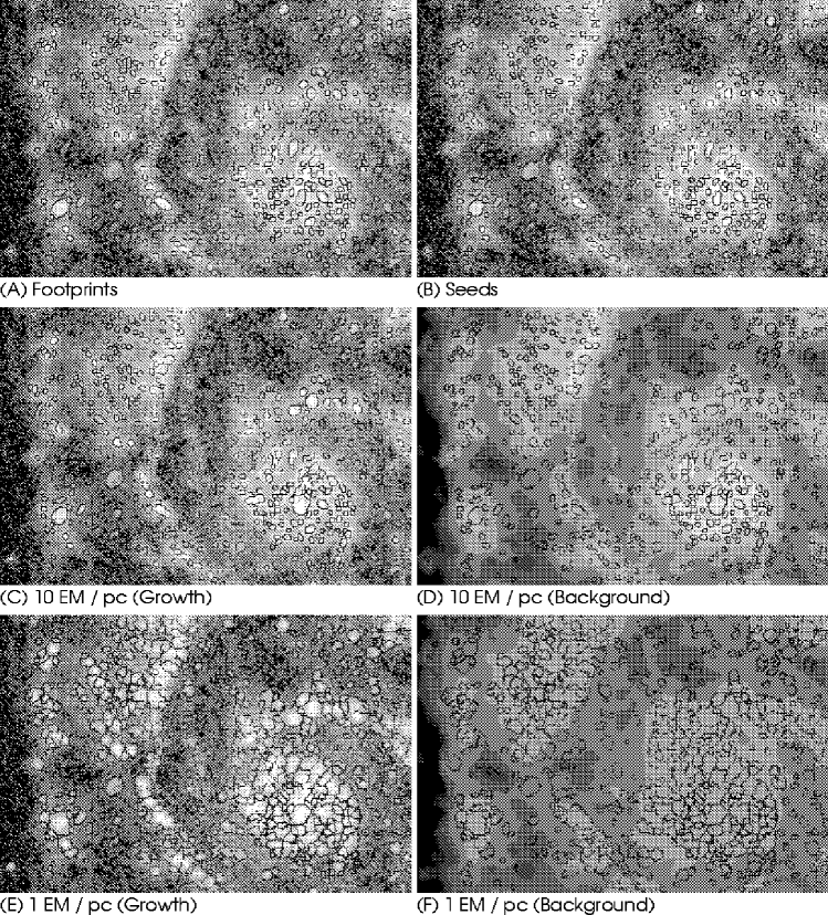
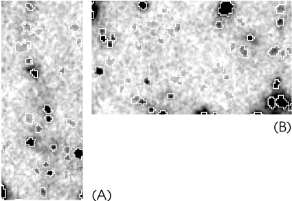
Figure 2 illustrates the complete HIIphot procedure by showing the same image section within a continuum subtracted H$\alpha$ image of M51 at various stages of the processing. In particular, Fig. 2a shows our HIIphot footprints. The image data has been scaled logarithmically to keep from saturating the inner portions of the galaxy. Scaling is identical in each panel so as to facilitate comparison between panels 2c–2f. All marked regions are associated with a convolution peak ($5\sigma$ or better) at either original or somewhat degraded resolution. Fig. 3 shows two small subsections of Fig. 2c (see description further below) with linear scaling in order to demonstrate the significance of low surface brightness detections which are difficult to appreciate in Fig. 2. Not all of the detections shown in Fig. 3 are used in the construction of our H II region LF, as we demand that every “photometric source” have a final signal-to-noise ratio in excess of five. Nevertheless, all detections plotted are thought to be genuine, having been originally discovered using HIIphot and later confirmed by visual inspection of individual continuum-subtracted images (before CR-rejection) viewed at various resolutions. Recall that we never make use of (and draw no conclusions from) these intrinsically questionable detections. Essentially they should be considered candidates, until deeper observations become available.

Figure 2: Subsection of M51 shown at various stages of the HIIphot procedure. Panel (a) contains a continuum-subtracted H$\alpha$ image with “footprint” boundaries indicated. In panel (b), we present the same image with “seed” boundaries marked. Panel (c) indicates the extent of each region after growth to a terminal surface brightness slope of 10 EM/pc. Panel (d) shows a surface fit to the diffuse background emission remaining after growth to the state presented in panel (c). This type of fit is used to make corrections to the integrated flux of each H II region. Panel (e) indicates the maximum extent ever allowed by the HIIphot growing procedure (1 EM/pc terminal slope). At this point, H II regions boundaries contain not only the classical H II region but also any associated DIG in the immediate vicinity. Panel (f) is a fit to the slowly-varying background emission after growth to the maximum extent.

Because our empirical models are only a first order approximation to actual source structure, footprints often contain pixels that are not bright enough to justifiably remain in the final boundary of the region. We account for this by rejecting all pixels which fall outside a “bounding isophote” defined by 50% of the median data value found within each footprint (where the median is measured relative to an estimated local background). We call these trimmed footprints “seeds” since they are composed of only those pixels destined to belong to a region, but do not yet reflect changes associated with the iterative growth procedure. Our procedure ensures that all seed boundaries follow isophotal contours within footprint boundaries, although the specific cutoff varies depending on the distribution of pixel intensities within any given H II region. Notice that this conservative approach makes it possible for ring-like footprints to reject pixels which fall within the object’s central surface brightness depression. Fig. 2b shows the HIIphot seeds for our subsection of M51. In practice, our particular implementation of the “seed” convention is motivated by the following arguments: (1) multi-pixel seeds provide a “head start” for the iterative growth process, making it easier to reliably separate adjacent regions, (2) defining seeds as a data-regulated subset of model footprints allows the first true excursion of region boundaries from our set of empirical models.

Figure 3: Two small sections of the image presented in Fig. 2c, redisplayed with high-contrast linear scaling to better show the faintest detected H II regions. As described in the text, this figure indicates boundaries for all detections, regardless of their final signal-to-noise ratio. All such detections do pass a $5\sigma$ cut in the multi-resolution FIND routine, but signal-to-noise may subsequently drop as regions grow into fainter areas for which noise is relatively more significant. Scientific analysis only uses sources for which ${\frac{S}{N}}_{final}\geq 5$, unless specifically stated otherwise.

2.3 Iterative growth of detections

Given a set of seed pixels associated with every H II region in a galaxy, it might seem a simple matter to iteratively add pixels to each region until reaching the maximum extent of all nebulae. In fact, the implementation of a well-behaved iterative growing algorithm is far from trivial and there is no established convention for determining the “edge” of an H II region. McCall, Straker & Uomoto (1996) encountered difficulty in growing their sources to isophotal cutoffs fainter than about 70% of the local peak. Potential inhomogeneity in the diffuse background level and crowding of regions having remarkably different flux conspire to make the PPP method less suitable except in a limited set of well-behaved circumstances. HIIphot attempts to carefully control the rate of growth in saddle points between regions by introducing a slowly declining threshold which determines the set of pixels considered for growth during a given iteration. Pixels having values below this global threshold are ignored until later iterations. In this way, neighboring regions approach their saddle point at an equal rate no matter what the difference in peak value or total counts between sources.

Iterative growth commences by setting the global threshold for pixel consideration equal to the highest bounding isophote and is reduced by 0.02 dex before each subsequent iteration. Regions as a whole are considered for growth only if the median value of the pixels in a seed’s “exterior perimeter” exceeds the slowly declining threshold. This implies that only the seed having the highest bounding isophote is considered during the first iteration. Any time that more than one region is allowed to grow during an iteration, HIIphot cycles through the active regions in order of decreasing correlation coefficient, $\rho$. Qualified pixels (lying above the global threshold) which are adjacent to or diagonal from any pixel already belonging to the region being augmented are potentially added to the source if they are not claimed by other regions. That is, pixels from the exterior perimeter of a region can be added if they are bright enough. We also require that at least 50% of the perimeter pixels are added during any given iteration. If this is not the case, we postpone growth until the global threshold declines further, so as to simultaneously add most of an entire isophotal ring. Growth for a particular region continues in this manner until either: (1) the observed surface brightness profile flattens sufficiently, or (2) no more qualified pixels can ever be reached due to being surrounded by other regions or because of the intrinsic data values. Note that regions can “stall” for many iterations and do not immediately cease growing just because neighbor pixels cannot be considered (as a result of the global threshold). In other words, our iterative procedure amounts to carefully adding lower isophotal contours to all qualified regions after specifically accounting for a slightly unequal start brought about by our adaptive definition of seed boundaries.

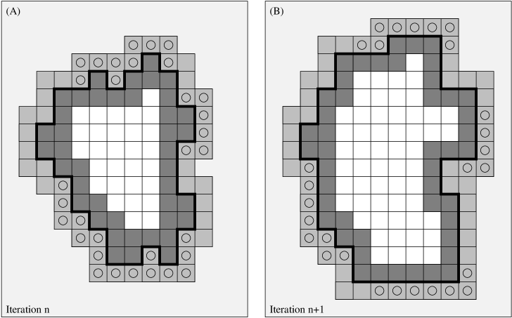
Figure 4 shows schematic representations of a hypothetical source being considered for iterative growth. In panel (4a), the dark shaded pixels belong to the region’s interior perimeter set during active iteration $n$, whereas lighter colored pixels compose the exterior perimeter group. The current region boundary is indicated with a heavy solid line. Median values for the interior/exterior perimeter sets will be used to determine if the surface brightness profile has flattened sufficiently in order to stop further growth (in subsequent iterations). Some of the lightly shaded pixels have been marked with a circle. These exterior perimeter pixels have values above the global threshold and will be added to the region during iteration $n$. Note that more than 50% of the lightly shaded pixels fall into this category. If this had not been the case, growth for this region would stall until the HIIphot global threshold declined enough to allow a majority of the exterior perimeter pixels to augment the region. Panel (4b) is similar to Panel (4a), except that it has been drawn for the following iteration, $n+1$.

Figure 4: Schematic representation of a hypothetical H II region undergoing iterative growth. We indicate the instantaneous boundary of the source with a heavy solid line. Pixels belonging to the “interior perimeter” set are shaded dark, whereas the “exterior perimeter” set is lightly filled. Members of the exterior set which exceed the global threshold for growth during each iteration are marked with circles.

The question of how to determine whether a surface brightness profile has “flattened” is somewhat difficult to treat on anything other than pragmatic grounds. Presently there is no established connection between the rate of surface brightness decline and specific physical conditions within an H II nebula. Originally we demanded that regions grow until the difference in median values between interior and exterior perimeter pixel sets indicated the surface brightness profile was no longer declining. This choice resulted in very large H II regions and significant bumping of adjacent regions, since in crowded fields brightness profiles rarely flatten out before encountering a neighbor. Our reason for requiring that the surface brightness profile flatten completely was that we sought to fairly treat all regions, regardless of their environment. Using this procedure we effectively determined groups of pixels most plausibly associated with the same ionizing source. That is, for this methodology, our H II “regions” included compact cores and related diffuse emission (DIG). Although interesting in its own right, this non-conventional definition of an H II region makes it difficult to compare the current results with previous work and we sought a more flexible alternative.

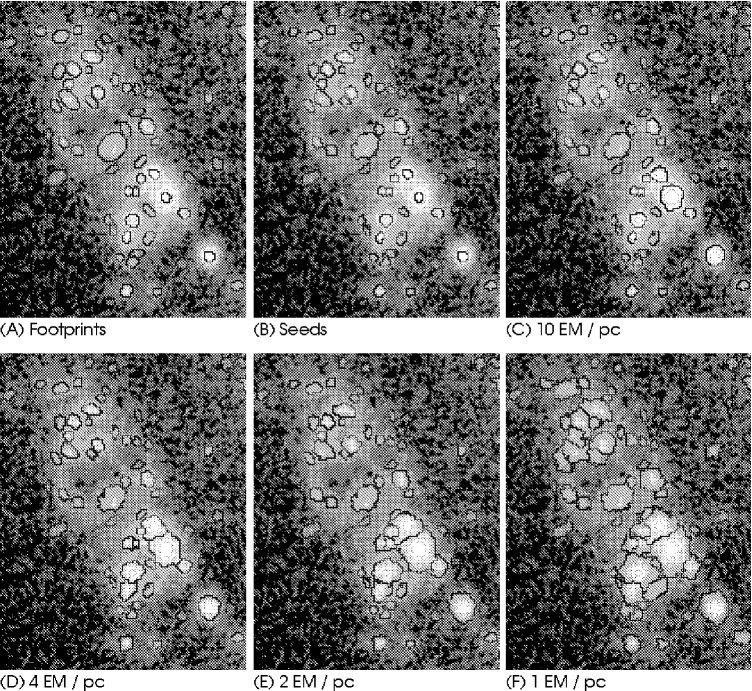
In the end, we elected to permit an array of different stopping points ranging from very little growth to nearly the generous “flat result” described above. This amounted to adopting a series of cutoffs in terminal surface brightness slope, [10, 4, 2, 1.5, and 1] EM/pc, then running the growth procedure from beginning to end for each. Notice that the specific cutoff values given here are only appropriate if the calibrated narrowband data are expressed in the conventional units of EM, cm^-6 pc, and must be rescaled for any other case. In section 4.2, we show that this approach allows us to directly address systematic uncertainty in H II region fluxes (and the resulting luminosity function) associated with our decision to stop growth at a given point. Figs. 2c and 2e present images of the M51 subsection with H II region boundaries marked for two different values of the terminal surface brightness slope. In Fig. 2c growth has stopped at a slope of 10 EM/pc, leaving a substantial fraction of diffuse emission possibly associated with discrete H II regions remaining outside the HIIphot boundaries. Fig. 2e shows the result for growth continuing until surface brightness profiles flatten to 1 EM/pc. Notice how isolated regions do eventually stop growing on their own, while the crowded central area has effectively been subdivided into numerous chunks (each plausibly associated with an embedded ionizing source). The behavior of the iterative growth procedure is further illustrated in Fig. 5, which shows another section of M51 at several stages of growth. For reference, all the results presented in this paper are based on a terminal profile slope of 1.5 EM/pc, midway between the degree of growth shown in panels (e) and (f) of Fig. 5.

Figure 5: Small continuum-subtracted H$\alpha$ subsection of M51, shown at various stages of the HIIphot procedure. In particular, panels (a) and (b) indicate the footprint and seed boundaries, while panels (c-f) show the gradual growth of detected H II regions. Panel (c) represents growth to a terminal surface brightness slope of 10 EM/pc. Panel (d) indicates the end state for growth to 4 EM/pc. The extent of all H II regions in panel (e) was determined by growing until we reach 2 EM/pc, just before our nominal stopping point when the surface brightness profile of each region has flattened to at least 1.5 EM/pc. See Fig. 6 for the nominal result, showing all of M51. Finally, panel (f) shows the resulting boundaries when growth is continued to 1 EM/pc in an attempt to recover any locally concentrated DIG possibly associated with each classical H II region.

One important advantage of adopting terminal surface brightness slopes (specified in physical units) is that our procedure is relatively robust to changes in signal-to-noise. One can think of other criteria for stopping growth that are not as reliable. For instance, we initially tried to quantify the “stopping point” for H II region growth in terms of various critical multiples of the formal error in the dimensionless surface brightness slope. This procedure appeared promising when analyzing our basic dataset, but was found to introduce substantial bias in the definition of H II region boundaries during experiments in which the signal-to-noise was globally reduced by factors ranging from 2 through 5. In short, as the test images were made noisier, growth stopped progressively sooner despite the fact that the underlying observed surface brightness profiles were no different. Our adopted procedure is substantially more well-behaved under these circumstances and generates luminosity functions which are statistically indistinguishable at all but the lowest luminosities. Sadly, loss of low luminosity sources is unavoidable with degraded signal-to-noise no matter how regions are grown.

2.4 Correction for underlying emission

For H II regions embedded in a background of diffuse ionized gas it is important to accurately estimate the DIG flux contribution to the observed counts within a region’s boundary. In past studies, most authors have gauged the background contribution by interactively selecting one or more positions near each H II region they thought to be representative of the level underlying the source. Our method works as follows: (1) after final region boundaries are available, we define as “background” pixels all those unclaimed pixels within a projected distance of 250 pc from the boundary of an H II region, (2) next we select a uniformly-spaced set of “control points” to represent these background data, only accepting those which are at least 75% surrounded by other background pixels within a circular domain of 250 pc diameter, (3) we then compute the median value of all background pixels within the domain of each control point, and (4) we finally compute a surface fit to these median values. Our surface-fitting procedure generates a low-order solution on small scales by interpolating between the 3 nearest control points at every position, but in a global sense the product is a very high-order surface. The result is essentially an image of the diffuse emission present in the original data and therefore represents an excellent means of quantifying the diffuse fraction in galaxies (e.g. Hoopes, Walterbos & Greenwalt (1996)). Note that we compute a different surface-fit for each requested version of the region boundaries, as the degree of iterative growth will influence pixel membership in background annuli and therefore the estimated background level for each emission line source. Figs. 2d and 2f show the diffuse background for the growth states illustrated in Figs. 2c and 2e, respectively. Note how the level of diffuse emission is estimated to be substantially lower in the second case.

2.5 HIIphot data products

The output of HIIphot consists of several images and one catalog detailing properties of all detected regions. The catalog tabulates the following quantities among others: ID#, right ascension, declination, pixel position, number of pixels contained by the region, effective FWHM, major axis FWHM, axial ratio, position angle, total flux after correction for background emission, $1\sigma$ uncertainty in total flux after correction, and the peak surface brightness inside the region. See Section 2.6 for a description of how total corrected flux and its error are calculated. Note that right ascension, declination, pixel position, and FWHM values refer to the best-fitting empirical model associated with each region, so from before region growth.

The images produced by HIIphot include: (1) a copy of the continuum-subtracted line image with the various “after growth” boundaries marked, (2) several versions of the background surface fit (corresponding to different levels of growth), and (3) integer maps delineating the position and extent of each footprint, seed, and grown region. These integer maps can be used for supplementary analysis if identically gridded images at different wavebands are available. Among the most obvious applications are computation of line ratios or equivalent width for emission line objects. Finally, the HIIphot user has the option of dumping postage stamp collages depicting each source in the catalog.

2.6 Flux determination and signal-to-noise in HIIphot

The background-corrected emission line flux of an H II region is computed using the continuum image ($C$), the line+continuum image ($L$), and our HIIphot surface fit to diffuse background emission remaining in the continuum-subtracted line image after growth of sources ($D$). In this derivation we assume that $C$, $L$, and $D$ remain in ADUs. Additionally, we require that no sky background has been subtracted from either $C$ or $L$. This is essential if photon noise is to be properly modeled during estimation of signal-to-noise. For region $i$ (composed of pixels $j={1~{}...~{}n_{i}}$) the background corrected emission line flux, $F_{i}$, is calculated as:

$$F_{i}=\sum(L_{ij}-S_{i}C_{ij})-\sum D_{ij},$$ (2)

where $S_{i}$ is the continuum scaling factor appropriate for region $i$. In practice we hold $S_{i}$ constant for all regions. The formal $1\sigma$ uncertainty, $\delta F_{i}$, associated with $F_{i}$ is given by the quadratic sum of standard deviations associated with individual terms of Eq. 2:

$$\delta F_{i}=\frac{\sum({\delta L_{ij}}^{2}+{S_{i}}^{2}{\delta C_{ij}}^{2}+{\delta D_{ij}}^{2})^{1/2}}{g}$$ (3)

As written here, the units of $F_{i}$ and $\delta F_{i}$ are ADUs, while $g$ is the gain in terms of electrons per ADU. To convert into physically meaningful units we multiply by an appropriate calibration factor. We assume that $C$ and $L$ are both essentially sky-noise limited, implying the following relations:

$$\delta L_{sky}=\frac{1}{g}\left(\frac{gX_{L}L_{sky}}{n_{L}}\right)^{1/2},{\rm and}$$ (4)

$$\delta C_{sky}=\frac{1}{g}\left(\frac{gX_{C}C_{sky}}{n_{C}}\right)^{1/2}.$$ (5)

In these expressions, $n_{L}$ and $n_{C}$ are the number of images (assumed to have comparable exposure) combined to create $L$ and $C$, respectively. Multiplicative factors $X_{L}$ and $X_{C}$ have values near unity or slightly higher in order to account for the possibility that read-noise may still make a small contribution to the noise budget in the HIIphot sky region. $\delta L_{sky},\delta C_{sky},L_{sky},$ and $C_{sky}$ are each measured within the sky region of the input images, implying appropriate values for $X_{L}$ and $X_{C}$. This information then constrains a photon noise model for the data, as we can fold $X_{L}$ and $X_{C}$ together with $g$ to represent an effective gain ($g_{L}=gX_{L}$ and $g_{C}=gX_{C}$) for $L$ and $C$.

Next, we estimate the level of noise per pixel in the brighter, interesting portions of $L$ and $C$. The relevant equations are:

$${\delta L_{ij}}^{2}=\frac{g_{L}L_{ij}}{n_{L}}~{}e^{-},{\rm and}$$ (6)

$${\delta C_{ij}}^{2}=\frac{g_{C}C_{ij}}{n_{C}}~{}e^{-}.$$ (7)

Eqns. 6 and 7 specify most of the terms in Eq. 3. Variance in the diffuse background level, ${\delta D_{ij}}^{2}$, is determined empirically on the basis of the measured standard deviation near control points used during the background fitting process. Note that we convert such measurements to electrons before computation of $\delta F_{i}$.

Two comments must be put forward at this point. Our assumption of sky-noise limited imagery is a conservative approach. By adopting Eqs. 4–7, we guarantee that $\delta L_{ij}$ and $\delta C_{ij}$ will always be predicted accurately or overestimated. If readnoise contributes substantially to the standard deviation of pixel values in the user-selected sky region, the measured values of $g_{L}$ and $g_{C}$ insure that it will contribute an identical fraction of the estimated noise-budget for pixels that are substantially brighter (due to observed emission from the object of interest). In reality, this is not the case – detector readnoise is independent of the observed pixel intensity. Overprediction of error terms ${\delta L_{ij}}^{2}$ and ${\delta C_{ij}}^{2}$ is the unavoidable consequence. Furthermore, we argue that our procedure for evaluating the source signal-to-noise ratio ($F_{i}/\delta F_{i}$), is more accurate than the traditional method based only on continuum-subtracted data, especially in the limit of bright continuum emission. Previous studies have usually gauged the standard deviation per pixel in one or more selected “sky areas,” then added this term in quadrature based on the number of pixels in a region. This implies that their estimated signal-to-noise is independent of the original observed datavalues. Identical sources located in various positions on top of a variable background of (continuum or line) emission will be assigned identical signal-to-noise, even though the true uncertainty increases for sources embedded in a bright background.

3 Narrowband observations of M51

We obtained narrowband images of the M51/NGC5195 system as part of a separate project concerning diffuse ionized gas (DIG) in spiral galaxies (Greenawalt (1998)). These data were obtained in 1992 March using the No.–1 0.9 m telescope at Kitt Peak. Three H$\alpha$ + [N II] and two [S II] images of 20 min integration were recorded in addition to a set of offband continuum exposures. The bandpass of each filter was approximately 75Å. Complete details concerning our observations and image reduction can be found in Greenawalt, Walterbos, Thilker & Hoopes (1998). For the present analysis a slightly different flux calibration was used. The continuum-subtracted image originally presented in Greenawalt et al. was calibrated by comparison with the photometric data of van der Hulst, Kennicutt, Crane & Rots (1988). An identical procedure was employed by Rand (1992) in a detailed study of 616 M51 H II regions. Because we sought to compare our photometry directly with Rand’s, we bootstrapped to his flux scale using a sample of 10 bright, moderately isolated H II regions. The magnitude of this recalibration amounted only to $\sim$10%, most likely attributable to the use of different regions by Rand and Greenawalt.

The 1$\sigma$ noise of our continuum-subtracted line image is at an H$\alpha$ emission measure (EM) of 9.9 pc cm^-6 at $1.8\arcsec$ FWHM resolution. This corresponds to a surface brightness of $2.0\times 10^{-17}$ erg cm^-2 s^-1 arcsec^-2, or 3.5 Rayleighs. Our noise implies a limiting (5$\sigma$) point source flux of $3.6\times 10^{-16}$ erg cm^-2 s^-1, or equivalently an H$\alpha$ luminosity of $3.9\times 10^{36}$ erg s^-1, neglecting any background confusion. For this calculation and the analysis below, we have assumed a distance of 9.6 Mpc to M51 (Sandage & Tammann (1974)). At this distance, the $1.8\arcsec$ seeing prevailing during our observations corresponds to a linear resolution of 84 pc. No correction was attempted for extinction, in order to facilitate comparison with earlier H II region surveys. In reality, van der Hulst, Kennicutt, Crane & Rots (1988) report on extinction toward a large sample of M51’s most luminous H II regions, finding about 2 visual magnitudes in most cases. This should be kept in mind when interpreting our results.

4 Results

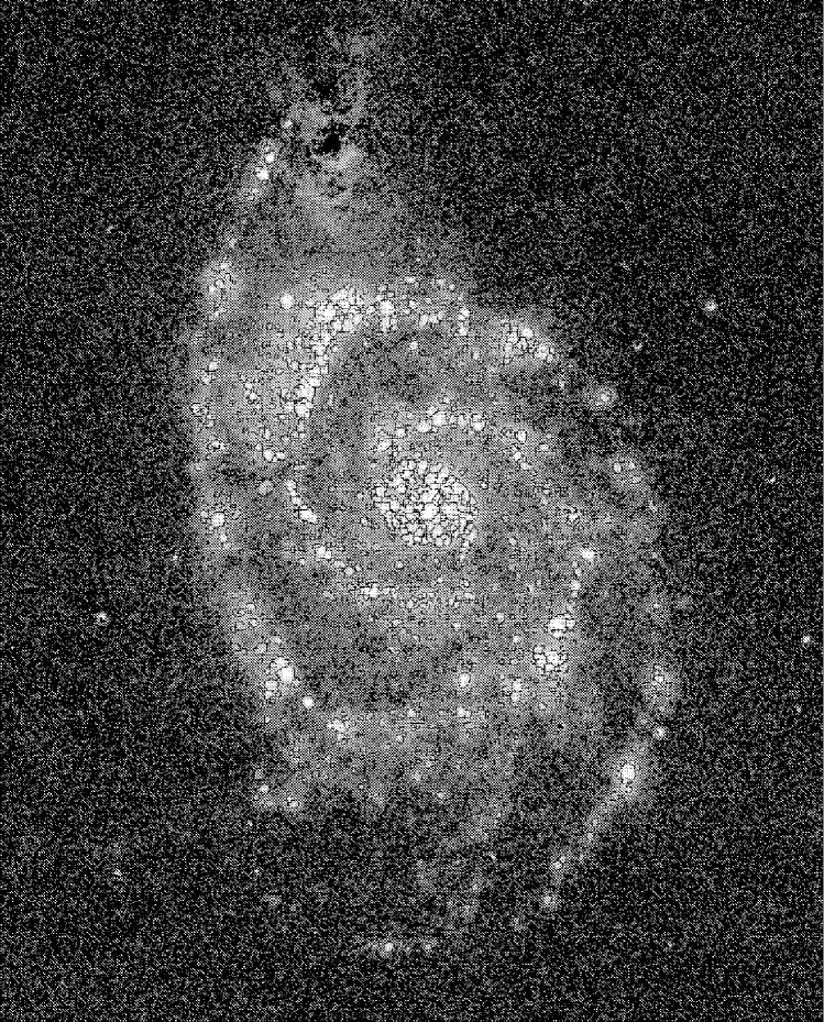
We detected 1618 H II regions in the field of view of our observations, excluding sources located in M51’s interacting companion NGC5195. Of the total sample, 1229 regions were classified as “photometric-quality” detections having ${\frac{S}{N}}_{final}\geq 5$. Only these 1229 H II regions have been considered in the analysis described below. Fig. 6 displays our continuum-subtracted H$\alpha$ image, with all source boundaries marked. Note that the extent of each H II region has been determined using a terminal surface brightness slope of 1.5 EM/pc. All results in the rest of the paper correspond to this choice, unless stated otherwise. The image has been logarithmically scaled in order to preserve contrast over a wide range in surface brightness. Notice the hand-drawn loop surrounding NGC 5195. It indicates the region specifically excluded from our M51 HIIphot survey.

Figure 6: Continuum-subtracted H$\alpha$ image of M51, with 1.5 EM/pc HIIphot boundaries indicated. The image has been logarithmically scaled in order to preserve useful contrast over the entire field. 1618 H II regions are marked, having luminosities in the range log L${}_{H\alpha}\sim 36-40$. Of these, a total of 1229 sources have estimated H$\alpha$ luminosities determined with at least 20% accuracy. Stellar residuals have not been blanked out, demonstrating the ability of HIIphot to ignore such image defects.

4.1 Overall comparison with R92

In this section we compare our H II region catalog with the list compiled by Rand (1992), hereafter R92, based on visual inspection and classification. We highlight the overall correspondence between our results and those of R92, but also describe variations attributable to procedural differences. We include a look at catalog completeness as a function of luminosity and morphological properties.

The most straightforward comparison between both catalogs is the total number of detected H II regions. Our detection list encompasses the entire galaxy, even the outer disk and confused nuclear portions not considered by Rand, suggesting we should find more sources than previously reported. However, other competing factors need to be considered as well:

(1) During the definition of footprints, HIIphot considers if a set of neighboring peaks is best described as a collection of individual regions or should be grouped into one or more composite aggregations. R92 always classified each neighboring peak as a separate source.

(2) HIIphot is perfectly consistent during the evaluation of marginal detections. Our estimate of signal-to-noise for each detection is evaluated on the basis of both the line+continuum and continuum datasets rather than just the continuum-subtracted line image (see Section 2.6).

(3) The catalogs were generated using images having different intrinsic sensitivity. The 1$\sigma$ noise in our data was $2.0\times 10^{-17}$ erg cm^-2 s^-1 arcsec^-2, whereas Rand’s imagery went down to $\sim 1\times 10^{-17}$ erg cm^-2 s^-1 arcsec^-2 (EM = 5 pc cm^-6), when evaluated at comparable spatial resolution.

(4) Contamination by emission-line objects other than traditional H II regions is a concern in our catalog. As a fundamental part of the R92 source selection process, each tentative detection was individually checked in a number of ways. Rand demanded that every source be centrally peaked, have a limited degree of circular symmetry, and possess a peak flux exceeding the background by more than 50%. HIIphot does not use any of these criteria. This means that our procedure is much more likely to result in a catalog containing “objects” such as localized enhancements in the widespread curtain of DIG, whether they be ionized on the spot by an embedded OB field star or by leakage from an H II region in a neighboring part of the galaxy, possibly hundreds of pc away. We elected to accept detections of this sort for three reasons: (1) they are intrinsically interesting, (2) they have little effect on the derived slope of the H II region luminosity function, and (3) eliminating such detections from the catalog would either require human intervention or an extra a priori constraint on the properties of detected H II regions. Note that contamination by planetary nebulae is equally unlikely in the R92 and HIIphot catalogs, since they would be too faint at a distance of 9.6 Mpc. Vassiliadis, Dopita, Morgan & Bell (1992) show that in the Magellanic Clouds there are no planetary nebulae with log L${}_{H\alpha}>36$, suggesting that both H II region catalogs are probably uncontaminated by PNe.

In the range of galactocentric radius examined by Rand (1 kpc $<R_{g}<$ 15 kpc), he reported 616 individual H II regions. HIIphot detected 1184 H II complexes with fluxes $\geq 5\sigma$ in the same area. Some of these objects are composed of multiple components. Although the total number of regions tabulated by HIIphot is more than reported by R92, we find that the agreement is substantially better in the range log L${}_{H\alpha}>38.5$. Rand detected 67 H II regions of this luminosity class, whereas we have 80.

The astute reader might ask how many of the regions detected by HIIphot are exactly the same sources described by R92. We explicitly checked this issue, finding that HIIphot misses only 2 of the 616 regions of R92. At the position of these two sources, we inspected our data and found no evidence for a significant detection. Note that our assessment of correspondence between the R92 source list and the HIIphot catalog was completed by way of manual inspection. During this process we demanded not only positional agreement, but also similar size between detections considered as being one in the same. It is important to note that due to the different methods of photometry it is unlikely that most sources had exactly the same effective boundary.

Figures 7 and 8 present a comparison of the measured luminosities for the regions in common to both our catalog and the R92 source list. Fig. 7 shows that there is a clear correlation (having slope $\sim 1$) between the luminosities measured by Rand and HIIphot. A limited number of H II regions fall substantially below the main cloud of datapoints. These sources most likely represent cases in which HIIphot broke a single R92 detection into one principal H II region and a small number of fainter peripherial sources. Figure 8 more clearly indicates a very subtle systematic change in the ratio of HIIphot/R92 luminosities as a function of source strength. We find that HIIphot tends to return slightly higher flux levels for very faint sources in comparison to the measurements of R92. This trend only begins in earnest at luminosities well below Rand’s estimated completeness limit (at L${}_{H\alpha}\sim 10^{37.6}$ erg s^-1). As shown in the next section, this systematic bias and the inherent scatter in Fig. 7 has very little (if any) influence on the H II region LF.

Figure 7: Comparison of measured luminosities for 614 sources in common between our catalog and R92. The dashed line indicates the anticipated unit slope in the case of a perfect correlation. There is substantial scatter about this line, but very little systematic deviation is apparent.

Figure 8: Log ( L_HIIphot / L_R92 ) versus log L_R92. In this graph, a slight tendency for HIIphot to measure systematically higher fluxes for the faintest regions with respect to the measurements of R92 is apparent. The error bars represent $\pm$ 1$\sigma$, evaluated in bins of width 1.0 dex.

So what are the detections “missed” by R92? In the area surveyed by Rand, we find that $\sim$80% of the regions picked up by HIIphot (but not listed in R92) have an H${\alpha}$ luminosity less than $10^{37.5}$ erg s^-1. Morphologically it is clear why most of them were not included in R92 – often they are rather diffuse and/or elongated. Sometimes these faint sources fall in the bright halo of a more significant H II region. In this case, interactive inspection of our continuum-subtracted line image typically reveals a relatively compact source superimposed on the brighter neighbor.

4.2 The H II region luminosity function

Figure 9 presents a comparison of the R92 differential luminosity function and our HIIphot result for exactly the same sources. Above their turnover points, both luminosity functions can be modeled as power law distribution (as first suggested by KEH89). Using only the data for regions in bins with log L${}_{H\alpha}\geq 37.6$ (those thought to be complete in R92) and assuming the standard functional form,

Figure 9: Comparison of the R92 differential H II luminosity function (for M51) and our equivalent result, only plotting 614 regions for which direct correspondence between catalogs could be established. The dotted lines are for R92, whereas solid lines represent the HIIphot data. In both cases, we plot the best-fitting power-law function as a straight line. Only bins having L_Hα greater than 10^37.6 erg s^-1 were used in these fits. The histograms are essentially identical, illustrating that the HIIphot flux measurement procedure does not introduce any detectable bias.

$$dN(L)=AL^{\alpha}dL,$$ (8)

we find that $\alpha_{\bf{\rm H{\small II}{\it phot}}}=-1.60\pm 0.07$, whereas $\alpha_{\rm R92}=-1.66\pm 0.07$. (For these fits we assumed simple counting statistics in order to assign a variance to each value of the LF. The weights used during $\chi^{2}$ minimization were inversely proportional to the variance of each bin, essentially giving the most influence to bins with the highest number of detections and reducing the influence of under-populated bins. This procedure is appropriate as long as no bins suffering from incompleteness are included in the fit.) The fact that there is no significant difference between the results plotted in Fig. 9 indicates that our HIIphot flux measurement technique does not introduce bias into the observed H II region luminosity functions.

Restoring the regions ignored for our comparison with R92, Fig. 10 presents an observed LF for all 1229 of the M51 sources detected by HIIphot with $S/N_{final}\geq 5$. The weighted power-law slope for this distribution is $\alpha_{\bf{\rm H{\small II}{\it phot}}}=-1.75\pm 0.06$, including only bins for which log L${}_{H\alpha}\geq 37.6$. Notice the break in the power-law at a luminosity of 10^38.9 erg s^-1. Our results confirm that M51 has a Type II LF, as originally defined by KEH89. For the purpose of comparison, Fig. 10 also presents the differential luminosity function from R92 - including the 2 sources not detected by HIIphot (this explains the slight difference with respect to Fig. 9). Rand estimated that his LF was complete down to log L_Hα = 37.6. In the text below, we carefully address incompleteness in the HIIphot catalog. In any case, Fig. 10 shows that our observed LF is marginally steeper than reported in R92. This probably reflects the enhanced sensitivity of our procedure at low luminosities and for relatively diffuse H II regions.

Figure 10: Observed M51 H II luminosity function, obtained using HIIphot with the establishment of lower limit on signal-to-noise (${\frac{S}{N}}_{final}\geq 5$). In total, 1229 regions were measured with this degree of accuracy. The solid line is a weighted power-law fit to the bins having L_Hα greater than the inflection at log L_Hα = 37.6. The power-law distribution has $\alpha$ = 1.75 $\pm$ 0.06. Note the prominent break in the LF at log L${}_{H\alpha}\sim 38.9$. For comparison we also plot the R92 result with a dotted line.

Note that our H II LF is subject to a systematic uncertainty associated with our choice of when to stop growing regions. In particular, the observed LF slope varies substantially if growth is stopped early or allowed to continue until region surface brightness profiles are more nearly flat. The LF slope quoted above ($\alpha=-1.75$) was obtained by growing H II regions until a terminal surface brightness slope of 1.5 EM/pc. If we had instead adopted a 1 EM/pc cutoff, the LF slope would have been shallower ($\alpha\geq-1.7$). In the case of minimal growth, the LF slope approaches $\alpha=-1.9$. We view this systematic difference as more of a change in the definition of an H II region, rather than uncertainty in our nominal result. The key point is that this “bias” can be properly addressed in a study of a sample of spirals by adopting the same procedure for all galaxies.

4.3 Investigation of incompleteness and blending effects

It is important to assess incompleteness effects. We investigated systematic trends such as the loss of faint, or bright but relatively diffuse, H II regions using simulations in which artificial sources were added to our original images. These altered data were subsequently reprocessed using HIIphot.

Blending due to limited spatial resolution can induce catalog incompleteness in crowded environments and flatten the observed LF at the faint end. H II regions tend to be inherently clumpy in terms of their spatial distribution, especially along spiral arms. This implies that the distribution of artificial H II regions should not be uniform across an image, but instead that additional H II regions should be placed preferentially in areas having recent star formation. Two ways to achieve this result are described below:

(1) Select a representative subset of detected regions in a galaxy and permit limited random walks away from actual tabulated positions, adding an artificial H II region in each slightly-randomized location.

(2) Use our HIIphot surface fit to the diffuse emission throughout a galaxy as a weighting function for the probability of placing an artificial H II region in any particular spot.

We elected to use the second method, as it provided more flexibility. For comparison, we also produced simulated images in which we distributed artificial sources at random.

We sought to reflect the intrinsic morphological diversity of H II regions in the prescription employed to generate artificial H II regions, rather than just adding unresolved sources of varied luminosity. Our incompleteness testing procedure allowed 3 types of simulated H II region: (1) small elliptical Gaussians, FWHM${}_{eff}=100$ pc, of varied axial ratio and position angle; (2) large elliptical Gaussians, FWHM${}_{eff}=200$ pc, of varied axial ratio and position angle; and (3) background-subtracted copies of actual H II regions extracted from the original data (mean FWHM_eff = 134 pc), scaled down to varying flux levels. In all cases, photon noise was added to each source before adding it into the line+continuum image being modified. Note that all direct image modification was performed on line+continuum images, since they are the relevant “observable” data. Afterwards, continuum subtraction was performed to compute a modified continuum-free line image. HIIphot was run using the modified continuum-subtracted line image, the modified line+continuum image, and the original continuum image.

Fig. 10 suggests that our observed M51 H II LF might begin suffering from incompleteness for sources as bright as $\sim 10^{37.0-37.5}$ erg s^-1 (just above the turnover point). We chose to insert 100 artificial regions of each type at 5 distinct luminosity values, log$(L_{H\alpha})=36.2,~{}36.6,~{}37.0,~{}37.4$, and $37.8$. Obviously each combination of source type, luminosity, and spatial distribution was investigated during a separate trial. The goal was to reliably constrain the true (“corrected”) H II LF down to log$(L_{H\alpha})\sim 36.6$.

Because actual (and simulated) H II regions have a spatial extent defined by irregular boundaries, one cannot simply inter-compare center positions for each detection in order to determine if simulated H II regions have been recovered. Each simulated source was assigned a code indicating whether it was: (1) recovered cleanly, (2) recovered as a blend, (3) essentially unrecovered, but partially blended with one other region, (4) essentially unrecovered, but partially blended with multiple regions, or (5) completely unrecovered. Sources were considered to be “recovered” (codes 1 and 2) if a single detection boundary encompassed pixels that contained at least 2/3 of the inserted region’s footprint flux (above the 20% isophote of the simulated source), otherwise the source was labeled “unrecovered” (codes 3, 4, and 5). For successfully recovered sources, cleanliness of recovery was judged by the fraction of total detection flux contributed by the simulated H II region. If a simulated region contributed at least 50% of the total flux in a detection, then it was assumed to be a clean recovery (code 1). Otherwise, blended recovery was indicated (code 2). For unrecovered synthetic sources, we evaluated the number of neighboring detections claiming at least one pixel of the unrecovered source footprint. If no pixels belonging within the simulated region’s 20% isophote were part of an HIIphot detection, then the artificial source was considered completely unrecovered (code 5). Likewise, if one and only one HIIphot detection claimed a pixel belonging to the unrecovered source footprint, the synthetic source was labeled essentially unrecovered, single blend (code 3). If more than one detection claimed a synthetic footprint pixel, then code 4 (multiple blend) was indicated. As a tool for determining the dependence of recovery statistics and photometric accuracy on variations in the local environment, we also classified the degree of crowding in the vicinity of each simulated H II region.

Before discussing the results of our completeness testing procedure, we note that the simulations provide a way to quantify the accuracy of our photometry as a function of luminosity. Because we know the exact flux of all simulated regions added to an image, we can determine the standard deviation of flux measurements for cleanly recovered sources. We examined the distribution of fractional flux discrepancy, defined as $(F_{observed}-F_{true})/F_{true}$, for each cleanly recovered artificial source without close neighbors. We find that the standard deviation of fractional flux discrepancy increases with decreasing source luminosity (as expected), ranging from 0.1 for log$(L_{H\alpha})=37.4$ up to 0.3 for log$(L_{H\alpha})=36.6$. Fractional flux discrepancy values were negligible for log$(L_{H\alpha})\geq 37.8$. The measurement scatter is significantly reduced for small sources. Furthermore, the median value of fractional flux discrepancy is very near zero for all but our faintest artificial sources.

Tables 1 and 2 present the end results of our completeness testing procedure for M51. Specifically, we have tabulated the percentage of simulated detections falling in each of the five recovery categories for all region types and luminosity values. Table 1 indicates the values for source placement via weighting the distribution of artificial sources to regions of star formation, while Table 2 shows what was recovered for the uniform source distribution.

As expected the simulations indicate our H II LF begins to be substantially incomplete by log L_Hα = 37.4 (about $L_{H\alpha}/L_{H\alpha,RMS}=32$). At this luminosity, nearly one third of the “actual” variety synthetic H II regions could not be recovered by HIIphot (see Table 1). We do find that small sources are easiest to recover. Large Gaussians were much more susceptible to blending with one or more sources. Actual regions appear to be intermediate – harder to recover than 100 pc Gaussians ($1.2\times$ PSF FWHM), but significantly easier than 200 pc Gaussians ($2.4\times$ PSF FWHM). These statements hold for both the weighted and uniform source distributions. Table 1, which shows the results for our weighted distribution tests, is most appropriate for the galaxy at large. However, the uniform distribution recovery statistics should be used when looking at completeness issues in uncrowded regions.

The results of our completeness testing procedure allowed us to perform Monte Carlo simulations designed to gauge systematic bias due to blending of faint, indistinct regions with brighter sources in observed luminosity functions. A separate paper will discuss the detailed findings of this investigation in a more general context. However, we were able to show that for the M51 completeness statistics (presented in Tables 1 and 2) the slope of the luminosity function above the low luminosity turnover was rather insensitive to “upward contamination” (see R92) potentially brought about via blending.

This result is actually somewhat of a coincidence related to the specific observed power law slope of the M51 LF. For intrinsically steeper luminosity functions, having $\alpha\sim-2.0$ for instance, blending can lead to a shift in the turnover point (to higher L) and create an artificial hump at slightly higher L (in excess of the true number of sources per bin). Shallower LFs than M51 are less susceptible to blending effects, but suffer severely from non-detection of low luminosity regions. For such systems, the turnover of the LF becomes rather broad and fitting a power law slope to bins just above the turnover leads to an underestimate of the true $\alpha$ (that is, we are fooled to think the LF is shallower than it actually is). As stated above, the M51 power law slope ($\alpha=-1.75$) is just shallow enough to avoid severe upward contamination, but not yet flat enough to substantially change the histogram character near the turnover point. Consequently, we conclude the observed M51 LF slope is rather robust to systematic bias and suspect that the true (unobservable) LF slope falls within the quoted uncertainty range for $\alpha$.

4.4 Distance-related effects on the observed LF

Systematic application of HIIphot to a large sample of galaxies will be able to address the effects of limited spatial resolution and sensitivity on observed H II region luminosity functions. Both of these observational characteristics are directly related to the distance for the object of interest. We can gauge the intrinsic bias related to limited resolution and sensitivity by deriving two LFs for each galaxy, one at the actual distance of the observed system and another using data which has been degraded to make the observations appear as if the galaxy was at the distance of our most-removed system. Although not really an issue in the present context, since we are studying a single galaxy which is already moderately distant (9.6 Mpc), this section has been included to demonstrate the technique and show that it is rather easy to realize given the HIIphot procedure.

We adopted a conservative procedure for generating image sets corresponding to the same galaxy at various distances. Instead of merely convolving the continuum-subtracted line image, then regridding, and adding noise (as is typically done), we independently transform the line+continuum and continuum images, only then creating the continuum-subtracted result. This procedure is required to accurately keep track of the photon statistics associated with continuum emission underlying H II regions. Neglecting this “hidden” noise may result in an overestimate of sensitivity when mimicking the effects of increased distance to a system.

The following step-by-step summary explicitly outlines our procedure:

(1) Select a “blank sky” region within the field of view of the continuum-subtracted line image.

(2) Determine the median level and standard deviation of this sky region in both the line+continuum and continuum images.

(3) Subtract the respective sky level from the line+continuum and continuum images.

(4) Determine the total number of galaxy counts in each image.

(5) Convolve with an appropriate Gaussian kernel (having peak of unity) in order to reduce the spatial resolution in both images.

(6) Regrid the convolved line+continuum and continuum images to a scale which results in the same PSF as the original data.

(7) Scale down the number of counts in each regridded image to be consistent with the totals determined in Step 4. That is, $F_{total,new}=F_{total,orig}({\frac{D_{orig}}{D_{new}}})^{2}$, where $D_{orig}$ and $D_{new}$ are the original and increased distances to the galaxy, respectively.

(8) Add the appropriate sky level back into each image.

(9) Based on the assumption that the original data were sky-noise-limited, add photon noise according to a model derived from our blank sky region (see Step 2). This model insures that the magnitude of simulated noise is higher in bright parts of the image.

(10) Using the distant images created in Steps 1-9, perform continuum subtraction to compute the line only image.

For the present demonstration, we generated datasets corresponding to the appearance of M51 at distances of 15, 30, and 45 Mpc (having PSF FWHM $\sim$ 130, 260, and 390 pc respectively). Fig. 11 shows a comparison of the H II LFs obtained by running HIIphot on these degraded data. The dotted line traces the actual observed M51 LF, presented earlier in Fig. 10.

Figure 11: Dependence of the measured H II region luminosity function on systematic effects related to distance, including reduced spatial resolution and sensitivity, is illustrated in this figure. We plot the M51 LF estimated from our original data (at full resolution) with the dotted histogram. After degrading the observations to simulate moving M51 to distances of 15, 30, and 45 Mpc, we reprocessed the images to derive the apparent LFs. These results are shown as dashed (15 Mpc), dash-dot (30 Mpc), and dash-triple-dot (45 Mpc) histograms in this plot. Histograms for original data, 15 Mpc, and 30 Mpc are vertically offset by 1.5, 1.0, and 0.5 dex, respectively, in order to preserve clarity. Blending and reduced sensitivity shift the low luminosity turnover, flatten the general slope of the LF, and can boost the brightest detections to artificially high apparent luminosities. Note, however, that even in the presence of these systematic effects the upper end LFs are remarkably consistent in regimes where all datasets are thought to remain complete (log L${}_{\rm H\alpha}\geq 38.6$).

Two effects are rather striking. The completeness limit at low luminosities increases in a smooth but dramatic fashion. Moving from 9.6 Mpc to 15 Mpc, the rapid loss of faint, isolated point sources takes place and our incompleteness limit (in this case judged by the LF turnover) rises slightly faster than one might expect according to the inverse square law. This effect is mitigated as the galaxy gets even more distant. Perhaps blending allows a small fraction of adjacent weak sources to be recovered as single (brighter) objects. The second striking effect shown in Fig. 11 is the influence of blending on the slope of the LF. It is clear that the LFs tabulated for 30 and 45 Mpc have substantially shallower power-law slopes than the 9.6 Mpc LF over a limited range of luminosity. Indeed, the best-fit LF slope ranges from $\alpha=-1.75\pm 0.06$ for the original data, to $\alpha=-1.22\pm 0.08$ for the case of M51 at 45 Mpc (fitting only sources with log L${}_{H\alpha}>38.0$). This effect is brought about by blending of H II regions (as spatial resolution is degraded) with some help from catalog incompleteness. Blending also explains the increased apparent luminosity of the brightest H II regions as the galaxy becomes more distant, although this effect is not illustrated by Fig. 11 (due to the choice of bin size).

It is worth noting that above a limiting luminosity, the original and degraded H II LFs are essentially identical within the errors. For this example, the completeness tests of Section 4.3 imply that all versions of the M51 data in Fig. 11 are complete above log L_Hα $\sim$ 38.6. In the few histogram bins above this limit, minimal difference between the various LFs is apparent.

4.5 Comparison of arm & interarm regions

The results of R92 included a demonstration of changes in H II region properties for those sources located in interarm gaps. We can classify arm/interarm status based on masking of the diffuse background image produced by HIIphot. Using this technique we confirm the difference in LF slope observed by Rand for arm versus interarm H II region populations.

A simple way to designate H II regions as belonging in the arm or interarm populations relies on masking of the HIIphot surface fit to the diffuse emission remaining after definition of H II region boundaries. These images typically show very conspicuous spiral structure. We experimented with several isophotal cutoffs to obtain a boundary that closely resembled that of R92. Although the present goal was to see if we could develop a masking technique to efficiently reproduce the classification scheme of Rand (who carefully subdivided the entire sample of H II regions on the basis of spiral arm morphology), a more appropriate characterization of our new method would be one in which the isophotal mask is used to segregate regions on the basis of their local star forming environment. Under the assumption that more DIG is found in areas of enhanced recent star formation, the “arm” H II regions identified by our mask could be thought of as sources that lie within especially active star forming areas of the galaxy. In the end, a cutoff at an H$\alpha$ EM of 30 pc cm^-6 worked well in both contexts for M51 (with $i=20\arcdeg$).

Fig. 12 shows the arm and interarm LFs created using the mask described above. The straight lines are weighted power-law fits to the data for H II regions brighter than log L_Hα = 37.6 and 37.0, for arm and interarm respectively. Our simulations of the previous section suggest that the catalog of interarm sources is complete to lower luminosities than the general population. This was the motivation behind choosing different lower limits for arm and interarm power-law fits. We find that there is a difference in slope between the two populations. The spiral arm population is best-fit with $\alpha=-1.72\pm 0.06$, whereas the interarm regions have a much steeper power-law slope given by $\alpha=-1.96\pm 0.15$. The brightest H II regions are found almost exclusively within the spiral arms. Only two interarm H II regions in M51 are more luminous than L_Hα = 10^38.1 erg s^-1.

Figure 12: H II LFs associated with spiral arm/interarm regions as classified on the basis of our EM masking technique. Notice the difference in power law slope for arm/interarm regions.

4.6 Correlation between H$\alpha$ luminosity and H II region size

We find that there is a correlation between the H$\alpha$ luminosity of a region and its projected surface area (PSA). Fig. 13 shows a plot of log L_Hα versus log PSA. Our data is best-fit by a line of slope 1.71, substantially higher than the predicted value of 1.5 for a classical (radiation bounded) Stromgren sphere of constant density. The scatter about the fit is rather large, especially for small H II regions. Note that we have chosen to present the correlation between log L_Hα and log PSA, rather than log of H II region effective radius (r_eff), because projected surface area is more directly related to our observations in the case of sources having irregular shape. We suspect that the slightly steeper than expected slope in Fig. 13 could be related to clumping within H II regions.

Figure 13: Correlation between log L_Hα and log (projected surface area) is observed for the H II regions of M51. The solid line shows a least absolute deviation fit to the datapoints and has slope 1.71, significantly higher than what one would expect for radiation bounded H II regions (slope = 1.5).

4.7 Characteristics of the DIG

The diffuse fraction in spiral galaxies remains of substantial interest for studies of ISM morphology and energetics. Defined as the ratio of DIG H$\alpha$ luminosity to total H$\alpha$ luminosity (Walterbos & Braun (1994)), the diffuse fraction has been estimated in a number of ways by different authors. The most common techniques are based on isophotal masking (e.g. Ferguson, Wyse, Gallagher & Hunter (1996), Hoopes, Walterbos & Greenwalt (1996), Wang, Heckman & Lehnert (1999)), although authors usually disagree on precise methodology. Classification of DIG has also been accomplished using explicit identification of traditional H II regions (Walterbos & Braun (1994)) and using maps of H$\alpha$ equivalent width (Veilleux, Cecil & Bland-Hawthorn (1995)). It is remarkable that the results obtained using diverse methods are quite similar, with a diffuse fraction of $0.4\pm 0.1$ being common for spiral galaxies (Greenawalt (1998)). Nevertheless, the diversity of methods employed makes it difficult to compare results in a detailed manner and accurately address relative uncertainties.

There are a few obvious drawbacks to each of the techniques previously used to estimate the diffuse fraction. In particular, inspection of the Fig. 2 in Ferguson, Wyse, Gallagher & Hunter (1996), Fig. 4b in Hoopes, Walterbos & Greenwalt (1996), and Fig. 8 in Greenawalt, Walterbos, Thilker & Hoopes (1998) reveals many instances of faint but highly localized H$\alpha$ emission being lumped into the DIG. These sources could be compact H II regions or even planetary nebulae. Attributing the flux of these faint discrete sources to DIG tends to artificially boost the diffuse fraction by a small (perhaps insignificant) amount. Secondly, several authors have pointed out that the total DIG luminosity should receive a contribution from locations in which H II regions are projected onto a slowly varying, diffuse background. The most commonly adopted solution is to assume that pixels occupied by an H II region each contribute the mean DIG intensity when totaling up DIG. This is undoubtedly an underestimate, as H II regions often have prominent DIG haloes, implying that the DIG superimposed on H II regions will typically be brighter than average. HIIphot addresses both of these problems, because it first measures flux associated with all discrete emission line sources and then individually estimates a background level for each region.

We calculate the diffuse fraction by independently totaling: (1) F_HII, the background-corrected flux associated with all detected H II regions (except those with ${\frac{S}{N}}_{final}<5$) , and (2) F_tot, the flux of the entire image. The diffuse fraction is then given by (F${}_{tot}-$F_HII)/F_tot. This is the method of Walterbos & Braun (1994), but accomplished in a repeatable automated manner. By computing the diffuse fraction for various requested stopping-points during the iterative growth process, we can accurately constrain the diffuse fraction and also place an upper limit on the amount of DIG ionized in the field, apparently unrelated to classical H II regions.

Using region boundaries established by our nominal 1.5 EM/pc terminal surface brightness slope, we find that the diffuse fraction for M51 is $0.45\pm 0.01$. The uncertainty quoted here only accounts for the possibility of variation in the sky background. Other uncertainties such as those associated with continuum subtraction and growth termination criteria will also play a role, as will flat-fielding errors. In fact, as described below, these factors may actually dominate the diffuse fraction uncertainty.

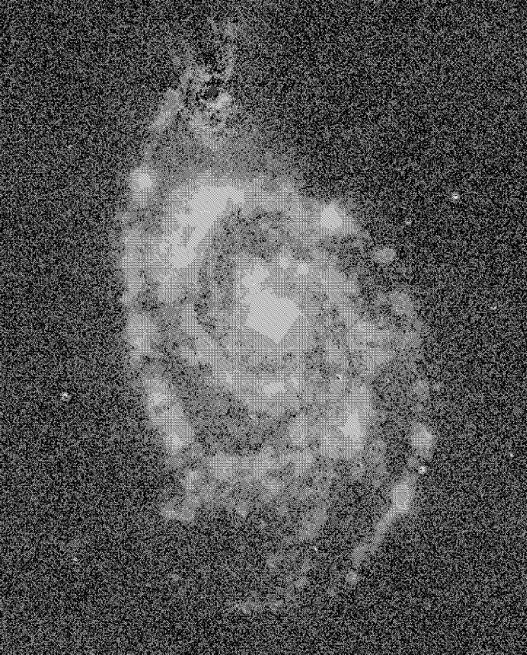
Just over half of the observed H$\alpha$ emission from M51 can be unambiguously associated with classical H II regions. Fig. 14 presents portions of our HIIphot surface fit to control points located in the diffuse emission not overlapped by H II regions. In this plot, we have only shown the diffuse background surface fit for pixels covered by an H II region - all other areas show the original data. Panels (d) and (f) of Fig. 2 present the entire smoothly varying surface fit for comparison. Note that there is still substantial spatial correlation between areas of bright DIG and obvious concentrations of H II regions. Indeed, bright rims around a significant number of H II regions can be seen in Fig. 14. Taken together, these facts seem to imply that we have not yet recovered all the H$\alpha$ emission which is powered by Lyman continuum photon sources inside traditional H II regions. It is entirely possible that our 1.5 EM/pc growth limit remains too conservative and should really be lowered if we want to accurately characterize the massive stars in H II regions.

Figure 14: Combination of the original continuum-subtracted image and the HIIphot surface fit to the diffuse background emission remaining after iterative growth. The diffuse surface fit has only been shown in regions coincident with detected H II regions. Note the clear spiral structure evident in this logarithmically scaled image. Images such as this are used to estimate the diffuse fraction over the entire galactic disk.

Figs. 2e and 5f represent the case in which H II regions were grown to encompass all apparently associated emission down to the sensitivity limit of the current data (by adopting a 1 EM/pc stopping point during the iterative procedure). Estimating the diffuse fraction with this set of region boundaries leads us to conclude that at most 38% of M51’s H$\alpha$ luminosity might originate via ionization by some mechanism other than leakage of Lyman continuum photons from H II regions. We do not mean to say that the conventional diffuse fraction is 0.38, but instead that a substantial fraction of the DIG emission in M51 cannot be plausibly tied to specific H II regions with the current data. This emission is still somewhat spatially correlated with the local density of H II regions, but ionization by “field” sources such as OB stars not in associations (Hoopes et al. 1999, in prep) may be largely responsible.

Our determination of the nominal diffuse fraction for M51 is clearly subject to systematic uncertainties related to our choice of the terminal surface brightness slope and uncertainty in the determination of the scale factor used during continuum-subtraction. Both of these can be empirically gauged. By computing the diffuse fraction immediately after growth commences (with a 10 EM/pc cutoff, see Fig. 5c), we obtain a hard upper limit of 0.68. At the very least, 32% of the H$\alpha$ emission from M51 is contained within the cores of classical H II regions. Systematic changes related to error in continuum-subtraction are easily measured by producing new versions of the line-only image then recomputing the background surface-fit and H II region fluxes. We generated “test” H$\alpha$ images by varying the continuum-subtraction scale factor $\pm$ 3% (1 $\sigma$) from our best-guess value. In the case of 1.5 EM/pc nominal growth boundaries, this resulted in diffuse fractions of 0.40 and 0.49, respectively for increased and decreased continuum emission.

We note in passing that the diffuse fraction is also potentially influenced by extinction variations across the face of a galaxy. The optical depth towards H II regions is probably elevated with respect to field DIG. Unfortunately, correcting for this systematic error would be rather difficult even in the case of measured Balmer decrements, given the unavoidable uncertainty in the geometry of emitting and absorbing volumes.

5 Summary

We have developed a new IDL procedure, which we have designated HIIphot, which is capable of performing fully-automated, repeatable photometry of H II regions. The procedure can detect and accurately characterize faint sources embedded in crowded fields, even in the presence of a substantially inhomogeneous, diffuse H$\alpha$ background.

In this paper we have applied HIIphot to the analysis of the grand-design spiral M51, studied previously by R92 and KEH89. Our results are in general agreement with these authors, although we detect more than twice the number of H II regions described by R92. In total, we find 1229 sources above $5\sigma$ having luminosity greater than about 10^36.1 erg s^-1. The LF obtained from this catalog of $5\sigma$ sources is reasonably well fit by a power law distribution having $\alpha$ = 1.75 $\pm$ 0.06, below a break in the observed number of regions near log L_Hα = 38.9. This break confirms the earlier classification of M51 as exhibiting a Type II LF.

In the near future, we plan to apply HIIphot for the analysis of an extensive galaxy sample for which high-quality, sensitive narrowband observations already exist. The sample will contain substantially more galaxies than observed by KEH89. Given the HIIphot code, it will be trivial to “reobserve” each of the galaxies at a common distance in order to inter-compare LFs in the absence of bias associated with different degrees of blending due to limited resolution and sensitivity. As a predecessor to this large study, we present HIIphot results for a smaller sample of 11 spirals in Thilker et al. (2000, Paper II). Therein we also develop a procedure for fitting HII LFs with predictions from population synthesis models of star cluster formation and evolution.

Table 1: Completeness evaluation results for weighted source distribution

Source	log $L_{H\alpha}$	$L_{H\alpha}/L_{H\alpha,RMS}$	Recovered	Recovered	Essentially	Essentially	Completely
type			cleanly	as a blend	unrecovered	unrecovered	unrecovered
					(single blend)	(multiple blend)
	(erg s-1)		(%)	(%)	(%)	(%)	(%)
100 pc Gaussian, $1.2\times$PSF	37.8	79	78	22	0	0	0
100 pc Gaussian, $1.2\times$PSF	37.4	32	67	30	0	3	0
100 pc Gaussian, $1.2\times$PSF	37.0	13	50	43	3	4	0
100 pc Gaussian, $1.2\times$PSF	36.6	5	27	59	2	10	2
100 pc Gaussian, $1.2\times$PSF	36.2	2	4	44	19	19	14
200 pc Gaussian, $2.4\times$PSF	37.8	79	43	25	0	32	0
200 pc Gaussian, $2.4\times$PSF	37.4	32	30	26	1	43	0
200 pc Gaussian, $2.4\times$PSF	37.0	13	21	14	5	60	0
200 pc Gaussian, $2.4\times$PSF	36.6	5	2	15	8	66	9
200 pc Gaussian, $2.4\times$PSF	36.2	2	0	18	11	66	5
Actual region	37.8	79	59	21	0	20	0
Actual region	37.4	32	40	29	0	31	0
Actual region	37.0	13	34	18	6	42	0
Actual region	36.6	5	9	31	12	43	5
Actual region	36.2	2	2	15	22	47	14

Table 2: Completeness evaluation results for uniform source distribution

Source	log $L_{H\alpha}$	$L_{H\alpha}/L_{H\alpha,RMS}$	Recovered	Recovered	Essentially	Essentially	Completely
type			cleanly	as a blend	unrecovered	unrecovered	unrecovered
					(single blend)	(multiple blend)
	(erg s-1)		(%)	(%)	(%)	(%)	(%)
100 pc Gaussian, $1.2\times$PSF	37.8	79	93	7	0	0	0
100 pc Gaussian, $1.2\times$PSF	37.4	32	82	18	0	0	0
100 pc Gaussian, $1.2\times$PSF	37.0	13	86	13	0	0	1
100 pc Gaussian, $1.2\times$PSF	36.6	5	47	43	3	5	2
100 pc Gaussian, $1.2\times$PSF	36.2	2	8	40	15	13	25
200 pc Gaussian, $2.4\times$PSF	37.8	79	67	7	1	25	0
200 pc Gaussian, $2.4\times$PSF	37.4	32	55	10	2	33	0
200 pc Gaussian, $2.4\times$PSF	37.0	13	23	21	11	44	1
200 pc Gaussian, $2.4\times$PSF	36.6	5	8	9	19	54	12
200 pc Gaussian, $2.4\times$PSF	36.2	2	0	13	22	47	21
Actual region	37.8	79	84	8	0	10	0
Actual region	37.4	32	68	15	0	17	0
Actual region	37.0	13	46	18	3	32	1
Actual region	36.6	5	23	16	21	30	10
Actual region	36.2	2	6	19	16	33	27

References

- Banfi, Rampazzo, Chincarini & Henry (1993) Banfi, M., Rampazzo, R., Chincarini, G. & Henry, R. B. C. 1993, A&A, 280, 373
- Evans & Dopita (1985) Evans, I. N. & Dopita, M. A. 1985, ApJS, 58, 125
- Feinstein (1997) Feinstein, C. 1997, ApJS, 112, 29
- Ferguson, Wyse, Gallagher & Hunter (1996) Ferguson, A. M. N., Wyse, R. F. G., Gallagher, J. S. , III & Hunter, D. A. 1996, AJ, 111, 2265
- Ferland, et al. (1998) Ferland, G. J., Korista, K. T., Verner, D. A., Ferguson, J. W., Kingdon, J. B. & Verner, E. M. 1998, PASP, 110, 761
- Greenawalt (1998) Greenawalt, B. E. 1998, Ph.D. Thesis, 16
- Greenawalt, Walterbos, Thilker & Hoopes (1998) Greenawalt, B., Walterbos, R. A. M., Thilker, D. & Hoopes, C. G. 1998, ApJ, 506, 135
- Hoopes, Walterbos & Greenwalt (1996) Hoopes, C. G., Walterbos, R. A. M. & Greenwalt, B. E. 1996, AJ, 112, 1429
- Kennicutt, Edgar & Hodge (1989) Kennicutt, R. C. , Jr., Edgar, B. K. & Hodge, P. W. 1989, ApJ, 337, 761
- Kingsburgh & McCall (1998) Kingsburgh, R. L. & McCall, M. L. 1998, AJ, 116, 2246
- Mashchenko, Thilker & Braun (1999) Mashchenko, S. Y., Thilker, D. A. & Braun, R. 1999, A&A, 343, 352
- McCall, Straker & Uomoto (1996) McCall, M. , Straker, R. W. & Uomoto, A. K. 1996, AJ, 112, 1096
- Oey & Clarke (1998) Oey, M. S. & Clarke, C. J. 1998, AJ, 115, 1543
- Osterbrock (1989) Osterbrock, D. E. 1989, Research supported by the University of California, John Simon Guggenheim Memorial Foundation, University of Minnesota, et al. Mill Valley, CA, University Science Books, 1989, 422 p.
- Rand (1992) Rand, R. J. 1992, AJ, 103, 815
- Sandage & Tammann (1974) Sandage, A. & Tammann, G. A. 1974, ApJ, 194, 559
- Stetson (1987) Stetson, P. B. 1987, PASP, 99, 191
- Stetson (1994) Stetson, P. B. 1994, PASP, 106, 250
- Thilker (1999) Thilker, D. 1999, Interstellar Turbulence, 104
- Thilker, Braun & Walterbos (1998) Thilker, D. A., Braun, R. & Walterbos, R. . M. 1998, A&A, 332, 429
- van der Hulst, Kennicutt, Crane & Rots (1988) van der Hulst, J. M., Kennicutt, R. C., Crane, P. C. & Rots, A. H. 1988, A&A, 195, 38
- Vassiliadis, Dopita, Morgan & Bell (1992) Vassiliadis, E., Dopita, M. A., Morgan, D. H. & Bell, J. F. 1992, ApJS, 83, 87
- Veilleux, Cecil & Bland-Hawthorn (1995) Veilleux, S. , Cecil, G. & Bland-Hawthorn, J. 1995, ApJ, 445, 152
- Walterbos & Braun (1994) Walterbos, R. A. M. & Braun, R. 1994, ApJ, 431, 156
- Wang, Heckman & Lehnert (1999) Wang, J. , Heckman, T. M. & Lehnert, M. D. 1999, ApJ, 515, 97
- Wyder, Hodge & Skelton (1997) Wyder, T. K., Hodge, P. W. & Skelton, B. P. 1997, PASP, 109, 927