Magnetic collimation of the solar and stellar winds

Abstract

We resolve the paradox that although magnetic collimation of an isotropic solar wind results in an enhancement of its proton flux along the polar directions, several observations indicate a wind proton flux peaked at the equator. To that goal, we solve the full set of the time-dependent MHD equations describing the axisymmetric outflow of plasma from the magnetized and rotating Sun, either in its present form of the solar wind, or, in its earlier form of a protosolar wind. Special attention is directed towards the collimation properties of the solar outflow at large heliocentric distances. For the present day solar wind it is found that the poloidal streamlines and fieldlines are only slightly focused toward the solar poles. However, even such a modest compression of the flow by the azimuthal magnetic field would lead to an increase of the mass flux at the polar axis by about 20% at 1 AU, relatively to its value at the equator, for an initially isotropic at the base wind, contrary to older and recent (Prognoz, Ulysses, SOHO) observations. For the anisotropic in heliolatitude wind with parameters at the base inferred from in situ observations by ULYSSES/SWOOPS and SOHO/CDS the effect of collimation is almost totally compensated by the initial velocity and density anisotropy of the wind. This effect should be taken into account in the interpretation of the recent SOHO observations by the SWAN instrument. Similar simulations have been performed for a five- and ten-fold increase of the solar angular velocity corresponding presumably to the wind of an earlier phase of our Sun. For such conditions it is found that for initially radial streamlines, the azimuthal magnetic field created by the fast rotation focus them toward the rotation axis and forms a tightly collimated jet.

Key words: Magnetohydrodynamics (MHD) – plasmas – Sun: solar wind – stars: pre-main sequence – stars: winds, outflows – ISM: jets and outflows

1 Introduction

Several stellar and extragalactic astrophysical systems have been observed to exhibit collimated outflows in the form of jets (young stellar objects, low and high mass X-ray binaries, black hole X-ray transients, symbiotic stars, planetary nebulae nuclei, supersoft X-ray sources, active galactic nuclei and quasars). In recent reviews of observations from all such classes of astrophysical objects it has been argued that an interconnecting element may be a rotating accretion disk threaded by a magnetic field (Livio 1999, Königl & Pudritz, 1999). Such connection between the disk and the jet is particularly evident in HST observations of several young stars in the nearby Orion nebula (Ray 1996). This rather convincing observational evidence of a close jet-disk relation is the basis for the presently prevailing view that an accretion disk is the necessary ingredient for the production of collimated jets.

On the other hand, theoretically it has been shown for quite some time by now that gas outflows from a rotating magnetized object of any nature can be magnetically self-collimated to form a jet (Heyvaerts & Norman 1989, Chiueh et al 1991, Sauty & Tsinganos 1994, Bogovalov 1995). This result seems to be a rather intrinsic property of magnetized winds with polytropic thermodynamics or not, where the self-compression of the plasma is provided by the toroidal magnetic field induced by the rotation of the central source. Henceforth emerges the generally accepted opinion that all observed jets are magnetically collimated (Livio 1999). However, no direct observational evidence exists today that most observed jets are indeed collimated solely by magnetic fields. Recently, it has been pointed out that the toroidal magnetic field is unstable and cannot collimate the jet effectively (Spruit et al. 1997, Lucek & Bell 1997) and it has been argued that magnetized winds do not collimate without an external help, such as the channelling effects of a thick accretion disk and/or confinement from the ambient medium (Okamoto 1999). It is thus crucially important to find direct observational evidence that the magnetic field mainly collimates the plasma in observed jets and by this way to test the theory of magnetic collimation.

Nevertheless, plasma outflows do also emanate from isolated magnetized and rotating stars without an accretion disk, of which the solar wind (SW) is the classical and best studied example. The natural question which arises then is to what observable degree dynamical effects are capable to collimate outflows from such single stars too. Theoretical studies on the angular momentum evolution of solar-type stars have concluded that at the end of the early accretion phase (PTTS) the star may be span up by more than 10 times the present solar rotation rate while its magnetic field is also strong (Bouvier et al. 1997). And, in recent studies it has been shown that cold winds from such rapidly rotating and highly magnetized stars lead to considerable collimation of the outflow (Bogovalov & Tsinganos 1999, henceforth Paper I). Similar is the result from studies of hot plasma outflows from efficient magnetic rotators (Sauty & Tsinganos 1994, Sauty et al. 1999). Hence, observation of the collimation effect in outflows from single stars could be the most reliable observational test of the theory of magnetic collimation.

The question of the degree of collimation of the SW is an interesting possibility that has not been fully answered theoretically and observationally for quite some time now. Suess (1972) and Nerney & Suess (1975) were the first to model the axisymmetric interaction of magnetic fields with rotation in stellar winds by a linearisation of the MHD equations in inverse Rossby numbers and to find a poleward deflection of the streamlines of the solar wind caused by the toroidal magnetic field. Later, Sakurai (1985) addressed the same problem by numerically solving the system of the polytropic MHD equations for the stationary outflow. Washimi & Shibata (1993) modelled time dependent axisymmetric thermo-centrifugal winds with a dipole magnetic flux distribution on the stellar surface and a radial field in Washimi & Sakurai (1993). Polytropic MHD simulations of magnetized winds containing both a ”wind” and a ”dead” zone (Tsinganos & Low 1989, Mestel 1999) have also been performed up to distances of 0.25 AU (Keppens & Goedbloed 1999). All these studies show some small deflection of the flow toward the axis of rotation.

In the observational front, information on the degree of collimation of the SW can be inferred from anisotropies in the Lyman alpha emission. These solar UV photons are scattered by neutral H atoms of interstellar origin and where the SW mass flux is increased the neutral H atoms are destroyed and thus the Lyman alpha emission is reduced. Early observations by the Mariner 10 (Kumar & Broadfoot 1979) and Prognoz (Bertaux et al. 1985) satellites have shown that there is less Lyman alpha emission near the equator in comparison to the ecliptic poles, than predicted by an isotropic SW (Bertaux et al. 1997). Therefore, these Lyman alpha observations imply that the SW mass efflux should be maximum at the equator and minimum at the poles. The same trend is confirmed by in situ observations of Ulysses (Goldstein et al. 1996) and the SWAN instrument onboard of the SOHO spacecraft (Kyrölä et al. 1998). However, the effect of SW collimation around the ecliptic poles would cause the opposite effect on Lyman alpha observations. In other words, although UV observations infer a SW mass efflux peaked at the equator, magnetic collimation would cause a SW mass efflux peaked at the poles, for an isotropic at the base wind.

One of the main purposes of this paper is to resolve this paradox. We shall follow the idea of magnetic collimation of the SW and show which values of the parameters characterizing the heliolatitudinal dependance of the SW (Lima et al. 1997, Gallagher et al. 1999), such as density, bulk flow speed, mass efflux, etc are consistent with the observations by the Lyman alpha method. Furthermore, we shall follow the increase of the degree of collimation of a hot stellar wind by increasing the rotation rate of the star and show that a ten-fold increase of angular velocity, as is the case in the majority of the young rapid rotators, leads to a dramatic increase of the degree of stellar wind collimation.

The paper is organised as follows. In Sect. 2 we justify the use of a split monopole model in our analysis for the collimation properties of the realistic solar wind at large distances from the Sun. In order to establish notation in Sect. 3 we give briefly the basic equations describing a stationary and polytropic Parker wind. In Sect. 4, the initial configuration used together with the boundary conditions for the numerical simulation in the nearest zone are discussed. In Sect. 5 the analytical method for extending the integration to unlimited large distances outside the near zone is briefly described while in Sect. 6 the parametrization of the presented solutions is given. In Sect. 7 we discuss the results for the isotropic SW in the near zone containing the critical surfaces and in the asymptotic regime of the collimated outflow, for a uniform rotation. In Sect. 8 the case of a stellar wind from a star rotating faster than the Sun is taken up. A brief summary with a discussion of the main results is finally given in Sect. 9.

2 The assumption of a split-monopole model for a stellar wind

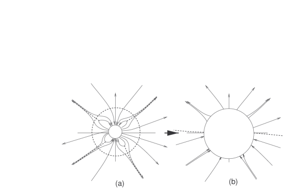
Fig. 1.: Schematic drawing of a white light image of the solar atmosphere indicating the shape of the solar magnetic fieldlines. Beyond the dotted spherical distance located around the slow magnetosonic critical surface the magnetic fieldlines are radial to a first approximation. Electric sheet currents are located on the dotted lines.

Fig. 1a is a sketch of the magnetic field structure in the corona of a star. Close to the stellar base the structure of the magnetosphere may be rather complicated. In this paper we are interested in the study of winds at distances much larger than the radius of the star where no closed field lines exist. It is therefore reasonable to consider the plasma flow starting at distances shown in Fig. 1a by the dashed line. For the solar wind the location of this surface can be put somewhere between the slow magnetosonic surface and the Alfvénic surface. We choose this location of the starting surface to avoid the solution of the problem of the wind acceleration in the very vicinity of the star which is defined not only by thermal pressure gradients but also by nonthermal processes of acceleration where the acceleration mechanisms have not still studied sufficienty well and are beyond the scope of the present study (e.g., see Holzer & Leer 1997, Hansteen et al. 1997, Wang et al. 1998). Above this base surface we can assume that the dynamics of the wind is mainly controlled by thermal and electromagnetic forces. In this approach the density and velocity of the plasma, together with the tangential components of the electric field and the normal component of the magnetic field are specified on this base surface while the tangential components of the magnetic field are free.

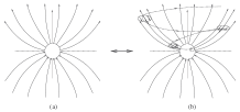
Fig. 2.: Plasma flow from an axisymmetric rotator with an initially split-monopole magnetic field, as in panel (a). Reversing the direction of the poloidal magnetic field in an arbitrary flux tube does not change the dynamics of the problem while we obtain the configuration shown in panel (b) which describes a nonstationary and nonaxisymmetric plasma flow from a rotator with a magnetic spot of opposite polarity on the base surface. The distribution of such spots can be arbitrary.

Nevertheless, the solution of this problem is still too complicated. Open poloidal magnetic field lines go to infinity and change their direction on the so called current sheets, some of which are indicated with dotted lines in Fig. 1a. These current sheets are present in any realistic wind from a stellar atmosphere, since the total magnetic flux of the open poloidal magnetic field lines is equal to zero while the mass loss rate is finite. The invariance principle summarized in the Appendix in a form appropriate to hot winds in a gravitational field allows us to simplify the structure of the magnetic field in the wind (Bogovalov 1999). According to this principle, we can reverse the direction of some field lines so that the magnetic field is unipolar in each hemisphere, e.g., outward in the upper and inwards in the lower hemisphere. In ideal MHD wherein we neglect all dissipative processes such as magnetic reconnection, this operation does not affect the dynamics of the plasma as long as the streamlines are not modified. This results in the configuration shown in Fig. 1b where since we are not interested in the region upstream of the base surface, this region is not shown. In this structure the current sheet is located only around the equatorial plane. To proceed, we further assume that the distribution of the normal component of the poloidal magnetic field is uniform in the upper and lower hemispheres. In that case we get the model of the axisymmetric rotator with an initially split-monopole magnetic field. The field lines are magnetically focused toward the system’s axis, as shown in Fig. 2a.

We would like to stress that the model of the axisymmetric rotator describes not only axisymmetric outflows but also a wide class of nonstationary and axially nonsymmetric outflows. This is due to the fact that according to the invariance principle (c.f. Appendix) the change of the direction of a magnetic field line in some flux tube does not affect the dynamics of the plasma. For example, let’s assume that we obtain a solution for the axisymmetric rotator, as shown schematically in Fig. 2a. Then, a reversal of the sign of some magnetic field lines in an arbitrary poloidal flux tube gives us a solution which is not axisymmetric and nonstationary, as shown in Fig. 2b. This is a solution for the plasma outflow from a rotator with uniform magnetic field at the base surface but with a magnetic spot of the opposite polarity on the upper hemisphere. Fig. 2b shows the cross-section of such a magnetic field by the poloidal plane. The stream lines are the same as for the axisymmetric case. But the poloidal magnetic field changes sign in magnetic spots corresponding to the flux tube of the opposite polarity. The path of the field line in this flux tube in 3D is shown by a dashed line. These spots propagate in the poloidal plane with the velocity of the plasma and hence the pattern is nonstationary.

It is clear that the number of such magnetic spots and their position at the base surface can be arbitrary. Therefore the study of the plasma outflow in the model of the axisymmetric rotator with an initially split-monopole magnetic field allows us to study a much more wider classes of nonstationary and nonaxisymmetric flows.

3 The stationary polytropic Parker wind

A Parker wind is taken as the initial state (t=0) for the solution of the time-dependent problem. In this initial state, the wind is assumed to flow along the radial magnetic field lines of an isotropic magnetic field (Parker 1963), although in general, the flow is not isotropic such that the wind has its own integrals of motion on every stream line $\psi=const$. For simplicity, a polytropic relationship between the pressure $P$ and the density $\rho$ is assumed

$$P=Q(\psi)\rho^{\gamma}\,,$$ (1)

where $\gamma$ is the polytropic index. Then, the Bernoulli equation for energy conservation along a radial line in such an anisotropic wind from a nonrotating star has the form

$${V^{2}\over 2}+{\gamma\over\gamma-1}Q(\psi)\rho^{\gamma-1}-{GM\over R}=E(\psi)\,.$$ (2)

Denote by $V_{\infty}(\psi)$ the terminal velocity of the plasma on each fieldline. In order to get equations in dimensionless variables, we shall use for the radial distance $\tilde{R}=R/R_{\rm s,eq}$, the density $\tilde{\rho}=\rho/\rho_{\rm s,eq}$, the entropy function $\tilde{Q}=Q/Q_{\rm eq}$ and the velocity $v=V/V_{\rm s,eq}$, in terms of the equatorial values of the sonic distance $R_{\rm s,eq}$, density $\rho_{\rm s,eq}$, entropy function $Q_{\rm eq}$ and sound speed $V_{\rm s,eq}$.

The mass flux conservation in these dimensionless variables takes the form

$$\tilde{\rho}v\tilde{R}^{2}={\dot{m}(\psi)}\,,$$ (3)

while the Bernoulli integral becomes,

$${v^{2}\over 2}+{\gamma\over\gamma-1}\tilde{Q}(\psi)\tilde{\rho}^{(\gamma-1)}-\left({GM\over V^{2}_{\rm s,eq}R_{\rm s,eq}}\right){1\over\tilde{R}}={v_{\infty}^{2}(\psi)\over 2}\,.$$ (4)

Since $v_{\infty}(\psi)$ can be regarded as a function of $\tilde{R}$ and $\tilde{\rho}$ along a particular streamline $\psi$, by taking the partial derivative of $v_{\infty}^{2}$ with respect to $\tilde{\rho}$ and $\tilde{R}$ we obtain the usual Parker criticality relations which give the sound speed $v_{\rm s}(\psi)$ and the spherical distance $\tilde{R}_{\rm s}(\psi)$ of the sonic critical surface along each streamline $\psi$ =const.,

$$v_{\rm s}^{2}(\psi)=\gamma\tilde{Q}(\psi)\tilde{\rho}_{\rm s}^{(\gamma-1)}(\psi)\,,$$ (5)

and

$$\tilde{R}_{\rm s}(\psi)={GM\over 2V^{2}_{\rm s,eq}R_{\rm s,eq}}{1\over v_{\rm s}^{2}(\psi)}\,,$$ (6)

with the lower index $s$ refering to the respective value of the variable at the sonic surface. Since, $\tilde{R}_{\rm s,eq}=v_{\rm s,eq}=1$ we have from the two criticality conditions,

$${GM\over 2V^{2}_{\rm s,eq}R_{\rm s,eq}}=1\,,$$ (7)

such that

$$\tilde{R}_{\rm s}(\psi)={1\over v^{2}_{\rm s}(\psi)}\,.$$ (8)

We are interested in obtaining the flow at large distances from the central source. Therefore we shall take the distribution of the velocity and mass flux at infinity as the input parameters of the problem and introduce the parameter

$$\xi(\psi)={V_{\infty}(\psi)\over V_{\rm\infty,eq}}\,.$$

Taking into account the above two criticality conditions we have,

$${v^{2}_{\rm s}(\psi)\over 2}+{v_{\rm s}^{2}(\psi)\over\gamma-1}-2v_{\rm s}^{2}(\psi)={v_{\rm\infty,eq}^{2}\xi^{2}(\psi)\over 2}\,,$$ (9)

which gives

$$v_{\rm s}^{2}(\psi)=\xi^{2}(\psi)\,,$$ (10)

and

$$v_{\rm\infty,eq}^{2}={5-3\gamma\over\gamma-1}\,.$$ (11)

Note that $v_{\rm\infty,eq}\geq 1$ only if $\gamma\leq 3/2$. The enthalpy function $\tilde{Q}(\psi)$ can be calculated in terms of $\xi(\psi)$ and $\dot{m}(\psi)$ from Eq. (3) evaluated at the sonic surface and Eqs. (8) - (5),

$$\gamma\tilde{Q}(\psi)={\xi^{2}(\psi)\over\tilde{\rho_{\rm s}}^{\gamma-1}(\psi)}={\xi^{5-3\gamma}(\psi)\over\dot{m}^{\gamma-1}(\psi)}\,.$$ (12)

From Eqs. (3) - (8), the density at the critical surface is given in terms of $\xi(\psi)$ and $\dot{m}(\psi)$,

$$\tilde{\rho}_{\rm s}(\psi)={\xi^{3}(\psi)\dot{m}(\psi)}\,.$$ (13)

The Bernoulli equation in dimensionless variables has the form

$${v^{2}\over 2}+{\xi^{5-3\gamma}(\psi)\over\gamma-1}\left({v\tilde{R}^{2}}\right)^{(1-\gamma)}-{2\over\tilde{R}}={5-3\gamma\over(\gamma-1)}{\xi^{2}(\psi)\over 2}\,.$$ (14)

The above Bernoulli equation determines the plasma flow $v(\tilde{R};\psi)$ along the prescribed radial magnetic field, once the polytropic index $\gamma$ and the distribution of the asymptotic velocity $\xi(\psi)$ are given. Then, Eq. (3) gives the density $\tilde{\rho}=\dot{m}/v\tilde{R}^{2}$ once the mass flux $\dot{m}(\psi)$ accross the poloidal streamlines is given. Note that in order to finally calculate the physical variables $V$ and $\rho$ we need in addition, as input parameter of the problem, the equatorial sound speed $V_{\rm s,eq}$ while $\rho_{\rm s,eq}$ can be calculated from the given $\dot{m}_{\rm eq}$.

Finally, consider the initial radial magnetic field

$$B=B_{\rm s,eq}\left({R_{\rm s,eq}\over R}\right)^{2}={B_{\rm s,eq}\over\tilde{R}^{2}}\,,$$ (15)

where $B_{\rm s,eq}$ is the magnetic field at the equatorial sonic transition. To define a dimensionless magnetic field, $\tilde{B}$, we need to normalize $B$ to some characteristic value $B_{\rm c}$ which we choose to be given by the condition $B_{\rm c}^{2}=4\pi\rho_{\rm s,eq}V_{\rm s,eq}^{2}$. The dimensionless magnetic field $\tilde{B}\equiv{B/B_{\rm c}}$ then has the form

$$\tilde{B}={B_{\rm s,eq}\over\sqrt{4\pi\rho_{\rm s,eq}}V_{\rm s,eq}}\left({R_{\rm s,eq}\over R}\right)^{2}={V_{\rm A,s,eq}\over V_{\rm s,eq}}{1\over\tilde{R}^{2}}\,,$$ (16)

where $V_{\rm A,s,eq}={B_{\rm s,eq}/\sqrt{4\pi\rho_{\rm s,eq}}}$ is the Alfvénic velocity at the equatorial sonic point. Evidently, the strength of the initial dimensionless magnetic field is controlled by the magnitude of the ratio of the Alfvén and sound speeds at the equatorial sonic distance, ${V_{\rm A,s,eq}/V_{\rm s,eq}}$.

4 The time-dependent stellar wind problem

To obtain a stationary solution of the problem in the nearest zone of the star containing the sonic critical surface, it is needed to solve the complete system of the time-dependent MHD equations and look for an asymptotic stationary state. Then, the plasma flow in a gravitational field with the thermal pressure included is described by the following set of the familiar MHD equations,

$${\bf B_{\rm p}}={\nabla\psi\times{\bf\hat{\varphi}}\over r}\,,$$ (17)

$${\partial\psi\over\partial t}=-V_{r}{\partial\psi\over\partial r}-V_{z}{\partial\psi\over\partial z}\,,$$ (18)

$${\partial\rho\over\partial t}=-{1\over r}{\partial\over\partial r}(\rho rV_{r})-{\partial\over\partial z}(\rho V_{z})\,,$$ (19)

$${\partial B_{\varphi}\over\partial t}={\partial\over\partial z}(V_{\varphi}B_{z}-V_{z}B_{\varphi})-{\partial\over\partial r}(V_{r}B_{\varphi}-V_{\varphi}B_{r})\,,$$ (20)

$${\partial V_{\varphi}\over\partial t} = -{V_{r}\over r}{\partial\over\partial r}(rV_{\varphi})-V_{z}{\partial V_{\varphi}\over\partial z}$$ (21)

$$+{1\over 4\pi\rho}\left(B_{r}{\partial\over r\partial r}(rB_{\varphi})+B_{z}{\partial B_{\varphi}\over\partial z}\right)\,,$$

$${\partial V_{z}\over\partial t} = -V_{r}{\partial V_{z}\over\partial r}-V_{z}{\partial V_{z}\over\partial z}-{1\over\rho}{\partial P\over\partial z}-{GMz\over R^{3}}-{1\over 8\pi\rho r^{2}}\times$$ (22)

$${\partial\over\partial z}(rB_{\varphi})^{2}-{B_{r}\over 4\pi\rho}\left({\partial B_{r}\over\partial z}-{\partial B_{z}\over\partial r}\right)\,,$$

$${\partial V_{r}\over\partial t} = -V_{r}{\partial V_{r}\over\partial r}-V_{z}{\partial V_{r}\over\partial z}-{1\over\rho}{\partial P\over\partial r}-{GMr\over R^{3}}-{1\over 8\pi\rho r^{2}}\times$$ (23)

$${\partial\over\partial r}(rB_{\varphi})^{2}+{V_{\varphi}^{2}\over r}+{B_{z}\over 4\pi\rho}\left({\partial B_{r}\over\partial z}-{\partial B_{z}\over\partial r}\right)\,,$$

where we have used cylindrical coordinates $(z,r,\varphi)$ and the magnetic field B has a poloidal magnetic flux denoted by $\psi(z,r)$. In the simulation we assumed a polytropic equation of state, so that the relationship of pressure and density in the plasma is $P=Q(\psi)\rho^{\gamma}$, at any point along the flow.

A correct solution of the problem requires a specification of the appropriate boundary conditions at the base surface. In this paper our main intention is to compare our results with observations at large distances from the source. In other words, we are interested in the asymptotic properties of the plasma flow in stellar winds. It is reasonable to start our numerical integration at a boundary surface $R_{o}$ placed just downstream of the slow mode critical surface. In this way we avoid the problems connected with the correct description of the acceleration of the flow below the slow mode critical surface. Nevertheless, our boundary sourface will be placed below the Alfvén and fast mode critical surfaces. The correct passage of the physical solution from these two critical surfaces will yield the appropriate values of the toroidal component of the magnetic field which is important in controlling the process of outflow collimation.

Then, the appropriate physical conditions at the boundary surface of integration are in dimensional variables:
1. The density of the plasma at $R=R_{o}$ kept constant in time, although it may depend on the colatitude $\theta$, $\rho=\rho_{o}(\theta)$.
2. The total plasma speed $V_{o}(\theta)$ in the corotating frame of reference at $R=R_{o}$, kept constant in time, although it may also depend on the colatitude $\theta$, $V_{(r,o)}^{2}+V_{(z,o)}^{2}+(V_{(\varphi,o)}-\Omega r_{o})^{2}=V_{o}^{2}(\theta)$ where $V_{o}(\theta)$ is the plasma speed on the surface $R_{o}$ of the initial flow. The value of the initial velocity $V_{o}(\theta)$ was taken such as to yield the observable values of the terminal velocity of the wind from a nonrotating star, i.e., typical solar wind velocities at 1 AU.
3. A constant and uniform in latitude distribution of the magnetic flux function at $R=R_{o}$, $\psi=\psi_{o}$.
4. Finally, the continuity of the tangential component of the electric field across the stellar surface in the corotating frame gives the last condition, $(V_{(\varphi,o)}-\Omega r_{o})B_{(p,o)}-V_{(p,o)}B_{(\varphi,o)}=0$.

Recently it was realized by Ustyugova et al. (1999) that the boundary conditions at the outer box of simulation are important for obtaining the correct physical stationary solution. The importance of a correct specification of the outer boundary conditions in MHD outflows has been emphasized previously in Bogovalov (1996, 1997) where we controlled the position of the outer boundary in the region where no signal can propagate from this boundary into the box of the simulation. For the solution of the full system of equations on the outer boundary we used only internal derivatives.

5 Method of numerical solution of the problem of stationary plasma flow to large distances from the star

The asymptotic solution of the time-dependent problem in the nearest zone containing the Alfvén and fast mode surfaces was used as the boundary condition for the far zone wherein we have a supersonic stationary flow. This boundary condition was then used in order to solve the system of the MHD equations describing the stationary outflow of superfast magnetosonic plasma. This system of equations consists of the set of the MHD integrals and of the transfield equation.

As is well known, the stationary MHD equations admit four integrals. They are the ratio of the poloidal magnetic and mass fluxes, $F(\psi)={B_{\rm p}/4\pi\rho V_{\rm p}}$; the total angular momentum per unit mass, $rV_{\varphi}-FrB_{\varphi}={L(\psi)}$; the corotation frequency $\Omega(\psi)$ in the frozen-in MHD condition $V_{\varphi}B_{p}-V_{\rm p}B_{\varphi}=rB_{\rm p}\Omega(\psi)$ and finally the total energy $E(\psi)$ in the equation for total energy conservation,

The method of the solution of the transfield equation in the super fast magnetosonic region is described in detail in our previous Paper I. An orthogonal curvilinear coordinate system ($\psi,\eta$) is used, formed by the tangent to the poloidal magnetic field line $\hat{\eta}=\hat{p}$ and the first normal towards the center of curvature of the poloidal lines, $\hat{\psi}=\nabla\psi/|\nabla\psi|$. A geometrical interval in these coordinates can be expressed as

$$(d{\bf r})^{2}=g^{2}_{\psi}d\psi^{2}+g^{2}_{\eta}d\eta^{2}+r^{2}d\varphi^{2},$$ (24)

where $g_{\psi},g_{\eta}$ are the corresponding line elements, i.e., the components of the metric tensor.

According to Landau & Lifshitz (1975) the equation $T_{\psi;k}^{k}=\rho{\partial\over\partial\psi}({GM\over R})$, where $T^{ik}$ is the energy-momentum tensor, will have the following form in these coordinates in the nonrelativistic limit,

$$\begin{array}[]{c}\displaystyle{{\partial\over\partial\psi}\left[P+{B^{2}\over 8\pi}\right]-{1\over r}{\partial r\over\partial\psi}\left[\rho V_{\varphi}^{2}-{B_{\varphi}^{2}\over 4\pi}\right]-}\\ \ \displaystyle{{1\over g_{\eta}}{\partial g_{\eta}\over\partial\psi}\left[\rho V_{\rm p}^{2}-{B_{\rm p}^{2}\over 4\pi}\right]=\rho{\partial\over\partial\psi}({GM\over R})}\,.\end{array}$$ (25)

It is convenient to solve the transfield equation in the system of the curvilinear coordinates ($\psi,\eta$) introduced above. The unknown variables are $z(\eta,\psi)$ and $r(\eta,\psi)$. Therefore we need to know the quantities $r_{\psi}$, $z_{\psi}$, $r_{\eta}$, $z_{\eta}$, where $r_{\eta}=\partial r/\partial\eta$, $z_{\eta}=\partial z/\partial\eta$, $r_{\psi}=\partial r/\partial\psi$, $z_{\psi}=\partial z/\partial\psi$ and $g_{\eta}$, $g_{\psi}$.

First, the metric coefficient $g_{\eta}$ is obtained from the above transfield equation (25),

$$g_{\eta}=\exp{(\int\limits_{a}^{\psi}G(\eta,\psi)d\psi)},$$ (26)

where

$${G(\eta,\psi)={{\partial\over\partial\psi}\left[P+{B^{2}\over 8\pi}\right]-\rho{\partial\over\partial\psi}({GM\over R})-{1\over r}{\partial r\over\partial\psi}\left[\rho V_{\varphi}^{2}-{B_{\varphi}^{2}\over 4\pi}\right]\over\left[\rho V_{\rm p}^{2}-{B_{\rm p}^{2}\over 4\pi}\right]}}\,.$$ (27)

The lower limit of the integration in (26) is chosen to be 0 such that the coordinate $\eta$ is uniquely defined. In this way $\eta$ coincides with the coordinate $z$ where the surface of constant $\eta$ crosses the axis of rotation.

The metric coefficient $g_{\psi}$ is given in terms of the magnitude of the poloidal magnetic field,

$$g_{\psi}={1\over rB_{\rm p}}\,.$$ (28)

To obtain the expressions of $r_{\psi}$, $z_{\psi}$, $r_{\eta}$, $z_{\eta}$ we may use the orthogonality condition

$$r_{\eta}r_{\psi}+z_{\eta}z_{\psi}=0\,,$$ (29)

and also the fact that they are related to the metric coefficients $g_{\eta}$ and $g_{\psi}$ as follows,

$$g^{2}_{\eta}=r_{\eta}^{2}+z_{\eta}^{2}\,,\penalty 10000\kern 3.0pt\penalty 10000\kern 3.0pt\penalty 10000\kern 3.0pt\penalty 10000\kern 3.0ptg^{2}_{\psi}=r_{\psi}^{2}+z_{\psi}^{2}\,.$$ (30)

Finally, by combining the condition of orthogonality (29) and Eqs. (30) the remaining values of $r_{\eta}$, $z_{\eta}$ are obtained,

$$r_{\eta}=-{z_{\psi}g_{\eta}\over g_{\psi}}\,,\penalty 10000\kern 3.0pt\penalty 10000\kern 3.0pt\penalty 10000\kern 3.0pt\penalty 10000\kern 3.0ptz_{\eta}={r_{\psi}g_{\eta}\over g_{\psi}}\,,$$ (31)

with $g_{\eta}$ above defined by the expression (26). For the numerical solution of the system of equations (31) the two step Lax-Wendroff method on the lattice with a dimension equal to 1000 is used.

Eqs. (31) should be supplemented by appropriate boundary conditions on some initial surface of constant $\eta$. The equations for $r_{\psi}$, $z_{\psi}$ defining this initial surface in cylindrical coordinates are,

$${\partial r\over\partial\psi}={B_{z}\over rB_{\rm p}^{2}},\penalty 10000\kern 3.0pt\penalty 10000\kern 3.0pt\penalty 10000\kern 3.0pt{\partial z\over\partial\psi}=-{B_{r}\over rB_{\rm p}^{2}}\,.$$ (32)

We need to specify on this surface the integrals $E(\psi),L(\psi),\Omega(\psi),F(\psi)$ as the boundary conditions for the initial value problem. To specify the initial surface of constant $\eta$ and the above integrals, we use the results of the solution of the problem in the nearest zone when a stationary solution is obtained for the time-dependent problem.

6 Parametrization of the stationary solution

It is convenient to consider the solution in dimensionless variables. In the present paper we express the velocities in units of the initial sound speed at the sound point on the equator $V_{\rm s,eq}$, all the geometrical variables in units of the initial radius of the sound point on the equator $R_{\rm s,eq}$ and the magnetic field in units of $B_{\rm c}=\sqrt{4\pi\rho_{\rm s,eq}}V_{\rm s,eq}$.

In this notation the solution depends on a few parameters. Among them is the ratio of the radius of the star to the radius of the initial sound point $\tilde{R}_{*}=R_{*}/R_{\rm s,eq}$, the parameters

$$\beta=\displaystyle{\Omega R_{\rm s,eq}\over V_{\rm s,eq}}\,,$$ (33)

and

$$V_{a}={V_{\rm A,s,eq}\over V_{\rm s,eq}}\,,$$ (34)

together with the two dimensionless functions $\xi(\psi)$ and $\dot{m}(\psi)$ which are equal to 1 in the case of uniform ejection of plasma at the base.

Since we are not interested here in the dependence of the solution on the radius of the star, basically the flow is defined by the two parameters $\beta$ and $V_{a}$.

Using the above definition of $\beta$ and the relationships at the critical surface, Eqs. (7) - (8), this parameter can be expressed through observable parameters as

$$\beta={\Omega GM\over 2V_{\infty}^{3}}({5-3\gamma\over\gamma-1})^{3/2},$$ (35)

where $V_{\infty}$ is the terminal velocity of the plasma for the nonrotating star with mass $M$. The parameter

$$V_{a}={\psi_{t}\over\sqrt{\dot{M}R^{2}_{\rm s,eq}V_{\rm s,eq}}}\,,$$ (36)

where $\psi_{t}=\lim_{r\rightarrow\infty}B\cdot r^{2}$ is estimated on the equator of the nonrotating star and $\dot{M}$ is the total mass loss of the nonrotating star.

In Paper I the degree of collimation of the outflow depended critically on a parameter $\alpha$ which was defined for cold plasmas as the ratio of the corotation speed at the Alfvén transition to the initial velocity of the plasma. However for hot winds where the velocity depends on the radial distance we should introduce a more general definition of this parameter $\alpha$.

In general, winds from astrophysical objects can be driven by a combination of several mechanisms of acceleration such as the gradients of thermal pressure, Alfvén wave and radiation pressures, magnetocentrifugal forces, etc. It is natural to characterize the efficiency of the magnetocentrifugal forces by the ratio $V_{m}/V_{\infty,0}$ where $V_{m}=({\Omega^{2}\psi_{t}^{2}/\dot{M}})^{1/3}$is Michel’s (1969) terminal velocity of a plasma accelerated only by magnetocentrifugal forces in the split-monopole model provided that the initial velocity is zero while $V_{\infty,\penalty 10000\kern 3.0pt0}$ is the terminal wind speed due to all other mechnisms of acceleration. In other words, $V_{\infty,\penalty 10000\kern 3.0pt0}$ is the terminal velocity of the plasma for the nonrotating star. In this case the generalized $\alpha$ can be defined as

$$\alpha=\left({V_{m}\over V_{\infty,0}}\right)^{3/2}\,.$$ (37)

In the special case of cold plasma outflow this definition of the parameter $\alpha$ coincides with the parameter introduced in our previous Paper I. It can be easily shown that for polytropic winds this parameter can be expressed as

$$\alpha=\beta V_{a}({\gamma-1\over 5-3\gamma})^{3/4}\,,$$ (38)

or,

$$\alpha={\psi_{t}\Omega\over\sqrt{\dot{M}}V_{\infty,0}^{3/2}}.$$ (39)

Magnetic rotators with $\alpha>1$ shall be called fast magnetic rotators and those with $\alpha<1$ slow magnetic rotators. It is useful to note that for a slow magnetic rotator such as the Sun, $R_{A}\approx\psi_{t}/(\dot{M}V_{\infty,0})^{1/2}$ (MacGregor 1996), and hence $\alpha\approx\Omega R_{A}/V_{\infty,\penalty 10000\kern 3.0pt0}$.

     

Fig. 3.: Shape of poloidal magnetic field lines and streamlines in the near zone of an isotropic (panel a) and anisotropic (panel b) solar wind with $\gamma=1.1$, $V_{a}=6.15$ and $\beta=0.165$. Spherical distance is given in units of radius of slow point at $R_{\rm slow}=8.4\penalty 10000\kern 3.0ptR_{\odot}$, with the base radius at $R=1.5$ (dashed line). Thick lines indicate slow, Alfvén and fast critical surfaces.

                 

Fig. 4.: Shape of poloidal magnetic field lines in the far zone of an isotropic SW with $\gamma=1.1$ and $\beta=0.165$. In (a) the poloidal field lines are plotted in a logarithmic scale, which magnifies their slight bending towards the axis, while in the linear scale of (b) it may be seen that collimation is negligible.

A quantitative classification of magnetic rotators on slow and fast (Belcher & MacGregor 1976) has also been introduced in Ferreira (1997) by using the parameter ${\Omega R_{A}/V_{A}}$, where $V_{A}$ is the Alfvén velocity in the Alfvén transition located at the radius $R_{A}$. This parameter is also less than 1 for slow rotators, but for fast rotators it is of the order of 1, since for fast magnetic rotators $V_{A}\sim\Omega R_{A}$ (Michel 1969). Nevertheless, physically this classification of magnetic rotators to fast and slow coincides in both cases. Note also in passing that in terms of an energetic criterion for collimation deduced in Sauty & Tsinganos (1994) and Sauty et al. (1999) magnetic rotators are analogously classified as efficient (with cylindrical asymptotics) and inefficient (with radial asymptotics).

7 Results for the isotropic and nonisotropic solar wind

The most often used magnetized polytropic solar wind model is the classical one proposed by Weber & Davis (1967) where the poloidal magnetic field and stream lines are radial (see also MacGregor 1996). This model reproduces the observed properties of the low speed streams at 1 AU within the observed fluctuations (Charbonneau 1995).

We will choose in our analysis the polytropic index to the value $\gamma=1.1$ such that the wind is heated. The spherical distance will be expressed in units of the distance of the slow magnetosonic point $R_{\rm slow}\approx 8.4\penalty 10000\kern 3.0ptR_{\odot}$ and the velocity in units of the slow magnetosonic speed there, $V_{\rm slow}\approx 106$ km/s. The fast magnetosonic transition occurs at $R_{\rm fast}\approx 38\penalty 10000\kern 3.0ptR_{\odot}$ where the fast magnetosonic speed is $V_{\rm fast}\approx 230$ km/sec. Note that for slow magnetic rotators like our Sun, the slow magnetosonic speed almost coincides with the sound speed and the Alfvén critical point with the fast magnetosonic critical point. In particular, at the axis the Alfvén and fast transitions coincide but at the equator the Alfvén transition occurs earlier as in Figs. 3 (see also Paper I and Keppens & Goedbloed 1999)

In Fig. 3a we plot the shape of the poloidal magnetic field lines and streamlines in the near zone of a wind which is isotropic at the base with $\gamma=1.1$, $V_{a}=6.15$ and $\beta=0.165$. With these parameters $\alpha=0.12$, i.e., in our terminology the Sun is a slow rotator. Careful inspection of this figure shows that the flow is very slightly collimated to the axis of rotation. The solution in the far zone is presented in Fig. 4.

In Fig. 4a the poloidal field lines of the SW are plotted in a logarithmic scale, which magnifies their slight bending towards the axis. This logarithmic scale extends to the huge distance of $10^{10}R_{\rm slow}$, i.e, about $4\times 10^{8}$ AU $\approx 60$ light years. This figure shows that the solar wind is indeed collimated toward the axis of rotation. But this collimation is indeed very weak. Fig. 4b shows the same field in a linear scale which shows that a jet is still not formed even at these huge distances.

                 

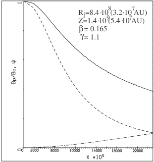
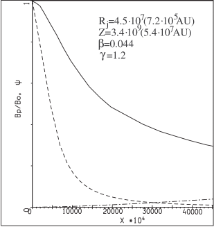
Fig. 5.: Variation with dimensionless cylindrical distance $X=r/R_{\rm slow}$ of enclosed magnetic flux $\psi(X)$ (dot-dashed) and magnetic field $B_{p}(X)/B_{o}$ (solid) for $\beta=0.165$ and $\gamma=1.1$ (panel a) and $\beta=0.044$ and $\gamma=1.2$ (panel b). Dashed line indicates the analytically predicted values of $B_{p}(X)/B_{o}$.

As is shown in Bogovalov (1995), the dependence of the magnitude of the poloidal magnetic field and density on the cylindrical distance $r$ becomes rather simple if we assume for convenience that the MHD integrals $E(\psi),L(\psi),F(\psi),\Omega(\psi)$ and the terminal velocity of the jet $V_{j}$ are constants and do not depend on $\psi$ and also that $V_{j}\gg V_{A}(0)$, where $V_{A}(0)$ is the Alfvénic velocity at the axis of rotation $r=0$. In such a case, an approximate estimate of the dependence of the magnetic field on $r$ is given in terms of the magnetic field and the density of the plasma on the axis of the jet, $B_{\rm p}(0)$ and $\rho(0)$, respectively,

$${B_{\rm p}(r)\over B_{\rm p}(0)}={\rho(r)\over\rho(0)}={1\over 1+(r/R_{j})^{2}}\,.$$ (40)

The radius of the core of the jet $R_{j}$ is given in terms of the sound and Alfvén speeds along the jet’s axis $V_{\rm s}(0)$ and $V_{A}(0)$,

$$R_{j}=\sqrt{\left(1+{V_{\rm s}(0)^{2}\over V_{A}(0)^{2}}\right)}{V_{j}\over\Omega}\,,$$ (41)

Hence, the poloidal magnetic field and density remain practically constant up to axial distances of order $R_{j}$ and then they decay fast like $1/r^{2}$ outside the jet’s core.

The comparison of this theoretical prediction with the characteristics of the solar wind is shown in Fig. 5. There is a remarkable discreapancy between them which tells us that even at these unrealistically huge distance (the SW wind is presumably terminated earlier) the jet has still not formed. The reason is that the collimation of the wind occurs logarithmically with distance (Paper I) provided that the jet is not formed in the nearest zone, as it happens for fast rotators. For the solar parameters, there isn’t enough radial distance to form the jet.

In spite of the absence of a jet core in the solar wind, the lines of the plasma flow are certainly bent to the axis of rotation. And some observable effects can arise due to this bending. If the base density is isotropic, the SW mass efflux increases with the latitude $\theta$ because of the magnetic focusing by about 20% from the equator to the pole (Fig. 6a) at a distance from the Sun of about 5.8 AU. Approximately at this distance the interplanetary $L_{\alpha}$ emission is formed, as observed by the SWAN instrument on board of SOHO. This theoretical anisotropy is in contradiction with the measurements of the anisotropy of the SW at large distance from the Sun by SWAN. This discreapency however, can be eliminated if we take into account some initial anisotropy in the SW.

To study in more detail the effect of the focusing of the SW, we peformed calculations for a more realistic model of the SW including some initial anisotropy of the wind at its base.

                 

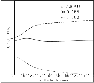
Fig. 6.: Distribution with latitude of characteristics of isotropic (panel a) and anisotropic (panel b) solar wind at 5.8 AU for $\beta=0.165$ and $\gamma=1.1$. Dashed lines indicate thermal pressure $P_{\rm th}(\theta)/P_{\rm th}(\theta=0)$, solid lines mass flux $J(\theta)=\rho vR^{2}$, dotted lines pressure of toroidal magnetic field $P_{\rm t}(\theta)/P_{\rm th}(\theta=0)$ and dotted-dashed lines pressure of poloidal magnetic field $P_{\rm p}(\theta)/P_{\rm th}(\theta=0)$.

In Fig. 3b the shape of the streamlines and Alfvén/fast critical surfaces is shown in the near zone of a wind which is latitudinally anisotropic in density and speed at the reference base at $R=1.5\penalty 10000\kern 3.0ptR_{\rm s,eq}$. For this simulation we used the latitudinal dependence of an exact MHD solution for the solar wind (Lima et al. 1997, Gallagher et al. 1999) with

$$\rho(\theta)={\rho_{0}}\left({1+\delta\sin^{2\epsilon}\theta}\right)\,,\;V_{r}(\theta)=V_{o}\sqrt{{1+\mu\sin^{2\epsilon}\theta\over 1+\delta\sin^{2\epsilon}\theta}}\,,$$ (42)

where $V_{0}$, and $\rho_{0}$ correspond to the reference values of the flow speed and density and the distribution depends on the three parameters $\delta$, $\mu$ and $\epsilon$. The values of $\epsilon$, $\delta$ and $\mu$ have been chosen in Lima et al. (1997) as to best reproduce the observed values of the wind speed at various latitudes, as obtained recently by Ulysses (Goldstein et al. 1996). Their deduced values which we adopted in this study are $\delta=1.17$, $\mu=-0.38$ and $\epsilon=8.6$. A similar density enhancement about the ecliptic and an associated increase of the wind speed around the poles is also found in recent MHD simulations as well (Keppens & Goedbloed 1999).

The distribution of the mass efflux at the distance of 5.8 AU for the anisotropic at the base SW is shown in Fig. 6b. The effect of the magnetic focusing almost totally disappers at high latitudes. Near the equator the excess of the mass efflux remains remarkable in the region below 30 degrees, although evidently the mass efflux decreases below 15 degrees. Therefore these results are in reasonable agreement with the distribution of the mass efflux of the SW which is deduced by SWAN at distances 5-7 AU.

The drastical decrease of the effect of the focusing of the solar wind in the anisotropic case can be naturally explained by the larger velocity of the SW at high latitudes. According to observations by ULYSSES, the velocity at high latitudes is almost twice higher than the velocity at the equator (Feldman et al. 1996). It follows from the equation of motion Eq. (25) that the curvature radius $R_{c}$ of the streamlines in the poloidal plane at large distances can be estimated as (Paper I)

$${1\over r^{2}}{\partial\over\partial\psi}{r^{2}B_{\varphi}^{2}\over 8\pi}\sim{\rho V_{p}^{2}\over rR_{c}B_{p}}\,.$$ (43)

The toroidal magnetic field at large distances can be estimated from the frozen in condition as $B_{\varphi}=-(r\Omega/V_{p})B_{p}$. In this case we have

$${1\over R_{c}}\sim{1\over 8\pi\rho V_{p}^{2}r^{3}}{\partial\over\partial\theta}\left({r\Omega\over V_{p}}\right)^{2}B_{p}^{2}r^{2}\,.$$ (44)

The latitudinal distributon of $\rho V_{p}$ is almost constant with an $\sim 15\%$ increase only near the equator. Therefore the curvature radius depends on $V_{p}$ as

$${1\over R_{c}}\sim{1\over V_{p}^{3}}\,,$$ (45)

provided that the mass flux density is fixed. Due to this strong dependence of the effect of collimation on the velocity of the plasma, the focusing practically disappears at high latitudes where the velocity is almost twice the velocity near the equator and the distribution of the mass efflux is in pretty good agreement with the observed one. The decrease of the mass efflux below $15^{o}$ cannot be found by the present SWAN data analysis since it was assumed in this analysis that the mass efflux can only monotonically increase with decreasing latitude.

Up to now we have discussed the results of calculations for the polytropic wind with $\gamma=1.1$. The flow with this polytropic index is almost isothermal and approximates the SW near the Sun, up to several dozens of solar radii. But at larger distances the effective polytropic index should increase and at infinity it should go to the Parker value $3/2$. At a first glance, it seems reasonable to expect that the focusing of the plasma will be stronger for a higher polytropic index.

To study this possibility we also performed calculations for the isotropic solar wind with a polytropic index $\gamma=1.2$, a reasonable value at the distance of several AU (Weber 1970). The change of the polytropic index results to a change of the other parameters $\beta$ and $V_{a}$ so that the total magnetic flux, mass flux and terminal velocity of the plasma remain constant as in the case with $\gamma=1.1$. In particular, for $\gamma=1.2$ we have $\beta=0.044$ and $V_{a}=11.9$. With these values of $\beta$ and $V_{a}$ the parameter $\alpha$ remains constant.

The distribution of the mass flux for $\gamma=1.2$ is shown in Fig. 7.

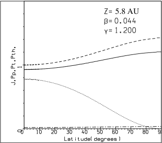
Fig. 7.: Distribution with latitude of the characteristics of the isotropic solar wind at 5.8 AU for $\beta=0.044$ and $\gamma=1.2$. Dashed line indicates thermal pressure $P_{\rm th}(\theta)/P_{\rm th}(\theta=0)$, solid line mass flux $J(\theta)=\rho vR^{2}$, dotted line pressure of toroidal magnetic field $P_{t}(\theta)/P_{\rm th}(\theta=0)$ and dotted-dashed line pressure of poloidal magnetic field $P_{\rm p}(\theta)/P_{\rm th}(\theta=0)$.

It follows from this figure that the focusing of the flow to the axis of rotation becomes even smaller at distances below 5.8 AU than it does for $\gamma=1.1$. This is explained by the fact that the higher is the polytropic index, the less is the variation of the plasma velocity with the distance. With a fixed terminal velocity, the wind with $\gamma=1.2$ has a higher velocity at the base than the wind with $\gamma=1.1$. But we already have discussed above the dependence of the focusing on the velocity of the flow. It follows from this discussion that the focusing is less for the wind with higher velocity. Therefore the focusing of the wind at several AU is maximal for $\gamma=1.1$. Since we have agreement of theory and observations of the solar wind anisotropy by SWAN for this polytropic index, it is expected that the wind with a higher polytropic index will not provide a higher level of collimation which could be inconsistent with the observations.

The dependence of the focusing effect on the polytropic index becomes opposite at very large distances where the plasma velocity has already achived the terminal value. In this case it becomes important how fast the thermal pressure which tends to decollimate the plasma falls down with distance. The higher the polytropic index is, the faster the pressure falls down with the distance. Therefore at very large distances we should expect stronger collimation of the plasma for higher values of the polytropic index. This tendency is indeed found. Fig. 5 demostrates a comparison of the characteristics of the flow near the axis of rotation for polytropic indices 1.1 and 1.2. It is seen that the wind for $\gamma=1.2$ is stronger collimated although the formation of the jets is also not completed at these huge distances.

     

Fig. 8.: Shape of poloidal magnetic field lines/streamlines in near zone of isotropic wind from a star rotating 5 times ($\beta=0.825$, panel a) and 10 times faster than the Sun, ($\beta=1.65$, panel b) for $\gamma=1.1$ and $V_{a}=6.15$. Spherical distance is in units of radius of slow point at $R_{\rm slow}=8.4\penalty 10000\kern 3.0ptR_{\odot}$, with the base radius at $1.5R_{\rm slow}$ (dashed line). The initial nonrotating monopole magnetic field has a spherical Alfvén surface at $4.5R_{\rm slow}$. Thick lines indicate slow, Alfvén and fast critical surfaces.

8 Stellar winds from magnetic rotators faster than the Sun

As we have seen in the previous section, the Sun is a relatively slow magnetic rotator with $\alpha<1$. A plausible senario for the Sun (and similar low mass stars) is that it has lost a large fraction of its angular momentum via magnetized a outflow while in its youth it was in a state of higher rotation, similar to the observed high rotation states of young stars (Bouvier et al. 1997) corresponding to larger values of $\alpha$. It is interesting then to examine the change of the shape of the magnetic field of a stellar magnetic rotator more efficient that the Sun, in the context of our simple modelling. For convenience and comparison with the present era Sun, we may keep constant the parameters of the polytropic index and sound speed. In rapid rotators, the magnetic flux also increases roughly in proportionality to the rotation rate $\Omega$ (Kawaler 1988, 1990). For simplicity let us neglect this increase and assume that the ratio of the Alfvén and sound speed remains the same, $V_{a}=6.15$, as in the previous example, but the parameter $\beta$ increases by 5 and 10 times, from $\beta$ = 0.165 ($\alpha=0.121$) to $\beta$ = 0.825 ($\alpha=0.6$) and then to $\beta$ = 1.65 ($\alpha=1.21$).

We shall again consider in our numerical experiment that the star has a radial magnetic field and at t=0 rotation starts which via the Lorentz forces distorts this magnetic field. After some time, a final equilibrium state is reached (Figs. 8) where the poloidal magnetic field and the plasma density are increased along the axis because of the focusing of the field lines towards the pole. A test that the steady state solution is reached is the constancy of the MHD integrals of motion, $E(\psi),L(\psi),F(\psi)$ and $\Omega(\psi)$. Note that the wiggles appearing at the midlatitude in Figs. 8 are due to the step-like function representation of the surface of the star in the cylindrical coordinate system used in our calculations. This artifact is unavoidable in this system of coordinates and is also present in the calculations reported in Washimi & Shibata (1993).

The shape of the poloidal field lines is shown in the near zone in Fig. 8. Collimation of the plasma to the axis of rotation already close to the source is evident. As in the cold plasma case of Paper I, the elongation of the subsonic region along the axis of rotation is present. The most surprising result is that this elongation occurs faster with an increase of the parameter $\alpha$ than it does for a cold plasma. It is easy to compare the flow in the nearest zone for $\alpha=1.2$ shown in Fig. 8b with the corresponding figure for similar $\alpha$ presented in Fig. 2 of Paper I. It appears that although the shape of the field lines is the same, the subsonic region for the cold plasma remains almost spherical at this parameter in contract to the shape of the subsonic region for the hot plasma. The physics of this interest behaviour is as follows.

The Alfvén transition at a given point of the Z-axis occurs when $V=(B_{p}/4\pi\rho V)B_{p}$. The ratio $B_{p}/\rho V$ remains constant along a field line. Therefore the right hand side in this expression increases with collimation as $B_{p}$. In the cold plasma limit $V$ is constant and the displacement of the Alfvén point down the flow in the cold plasma occurs only due to an increase of $B_{p}$. In the hot plasma case, the collimation also modifies the velocity $V$.

Fig. 9.: Flow speed at the axis (solid) and the equator (dashed line) for wind from a star rotating 10 times faster than the Sun, with $\gamma=1.1$ and $\beta=1.65$.

This modification is shown in Fig. 9. The solid line shows the velocity at the axis and the dashed line shows the velocity at the equator. Collimation results in an decrease of the thermal pressure gradient. Therefore the thermal acceleration of the plasma becomes less efficient. The velocity of the plasma even slightly decreases due to the gravitation force. Therefore the Alfvén surface in the hot case elongates along the axis of rotation with an increase of $\alpha$, faster than it does in the cold plasma case. It is clear that at some value of $\alpha$ specific for every flow, the subsonic region near the axis will be elongated to infinity in the Z-direction. In the hot plasma this happens at smaller $\alpha$ than it does in the cold plasma case. This subfast region should be certainly unstable. Therefore, the plasma flow at these conditions cannot be stationary. Those jets with $\alpha\gg 1$ eventually should become turbulent with properties differing from the properties of the stationary jets found for $\alpha<1$. The physics of these jets should be examined in a separate study.

In Fig. 10 the shape of the poloidal fieldlines is shown for the case of the rapid rotator. Their bending towards the rotation axis is evident not only in the logarithmic plot of Fig. (10a) but also in the linear plot of Fig. 10b where a tightly collimated jet is formed already at a relatively small distance from the source.

                 

Fig. 10.: Shape of poloidal magnetic field lines for a wind from a star rotating 10 times faster than the Sun, with $\gamma=1.1$ and $\beta=1.65$. In (a) the poloidal field lines are plotted in a logarithmic scale, which artificially magnifies their bending towards the axis, while in the linear scale of (b) a higher degree of collimation in comparison to the corresponding case of Fig. 4b may be seen.

In Figs. 11 the poloidal component of the magnetic field is plotted together with the magnetic flux enclosed by a cylindrical distance $X$. The poloidal magnetic field $B_{p}(X)/B_{o}$ (solid line) is given in units of its reference value $B_{o}$, corresponding to the magnetic field at the symmetry axis $r=0$ and some reference height $Z_{o}=5\cdot 10^{8}$ for $\beta=0.825$ (Fig. 11a) and $Z_{o}=1.66\times 10^{6}$ for $\beta=1.65$ (Fig. 11b). The asymptotic regime of the jet is achived at these distances. The dashed curve gives the analytically predicted solution for the poloidal magnetic field $B_{p}(X)/B_{o}$, Eq. (42). Note that the agreement between the calculated and analytically predicted values of the radius of the jet is pretty good. It follows from this comparison that for these parameters we indeed achieve the distance where the jets are really formed.

                 

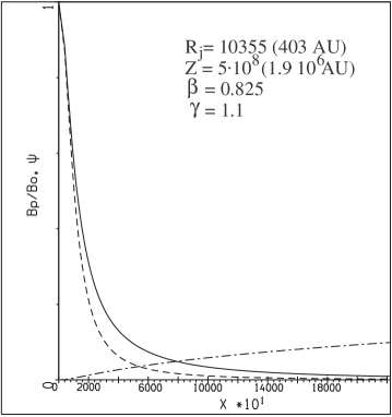
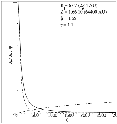
Fig. 11.: Variation with dimensionless cylindrical distance $X=r/R_{\rm slow}$ of enclosed magnetic flux $\psi(X)$ (dot-dashed) and magnetic field $B_{p}(X)/B_{o}$ (solid) from a moderate stellar magnetic rotator with $\beta=0.825$ (panel a) and a faster magnetic rotator with $\beta=1.65$ (panel b). Dashed line indicates the analytically predicted values of $B_{p}(X)/B_{o}$.

9 Discussion of the results

One of the basic results from the numerical simulations reported in this paper as well as in Paper I is that plasma ejected by rotating magnetized objects has the property of self-collimation. No other special conditions are needed to get a collimated outflow. Therefore, jets should be a rather common phenomenon in astrophysics. This is the most important prediction of the theory of magnetic collimation which is in pretty good agreement with observations, since numerous jets are observed to be associated with astrophysical objects of different nature.

However, a direct application of the theory of magnetic collimation to an isotropic solar wind predicts an increase of the mass efflux near the poles while observations of the distribution of the solar wind mass efflux with heliolatitude at distances 5 - 7 AU by a range of instruments have given the opposite result. In this work we eliminated this apparent contradiction by taking into account in the calculations more realistic parameters for the anisotropic solar wind, as those inferred recently by ULYSSES and SOHO. Then, a recalculation of the heliolatitudinal distribution of the SW mass efflux at large distances with an initially anisotropic distribution of the density and flow speed at the base show that the initial excess of the mass flux near the equator is preserved up to the outer boundary of the SW. Magnetic collimation is remarkable only in the region of the lower speed wind near the equator. It results in a relative decrease of the mass efflux in comparison with the flux at the low latitudes less than $15^{o}$. Can this effect be found in the SWAN data? To answer this question a detailed comparison of the calculations with these data is necessary.

It is widely believed that due to the observed close disk-jet connection collimated outflows are possible only from systems containing accretion disks. It is clearly demonstrated in this study that fast rotating stars without disks can also produce jet-like outflows. This prediction is crucially important for the theory of magnetic collimation, since it gives a most reliable observational test of the theory. Up to now there has been no direct observational evidence that observed jets are really collimated by the magnetic field. And, observation of jet-like outflows from objects which do not contain accretion disks would be this needed evidence.

Young fast rotating stars of solar mass are among the objects which produce jets. The effect of magnetic self-collimation of the winds is parameterized by $\alpha$, which can be presented in the form

$$\alpha=0.12{(\psi_{t}/\psi_{\odot})(\Omega/\Omega_{\odot})\over\sqrt{(\dot{M}/\dot{M}_{\odot})}(V_{\infty}/V_{\odot})^{3/2}}\,,$$ (46)

for $V_{\odot}\approx 400\penalty 10000\kern 3.0pt$ km/s. Some young stars with solar mass have angular velocities up to 100 times the angular velocity of the Sun (Bouvier et al. 1997). For example, in AB Doradus $\Omega_{\star}=54\penalty 10000\kern 3.0pt\Omega_{\odot}$ (Jardine et al. 1999). A phenomenological dynamo mechanism (MacGregor 1996) predicts a magnetic flux which scales as $\psi_{\star}/\psi_{\odot}\propto\Omega_{\star}/\Omega_{\odot}$. However, the dependence of the mass flux on $\Omega_{\star}$ is not known. The theoretical analysis in the Weber & Davis (1967) approximation shows that the mass flux is practically independent of the angular velocity. In such a case AB Doradus would have $\alpha\approx 350$. On the other hand, if the mass loss rate is proportional to the magnetic pressure, $\dot{M}_{\star}/\dot{M}_{\odot}\propto B^{2}_{\star}/B^{2}_{\odot}$, a value of $\alpha$ which is 54 times smaller results, i.e., $\alpha\approx 6.5$. This star is certainly a rapid rotator and should produce a collimated outflow. However, can such jets be observed ? Unfortunately their mass flux may be too small and thus it may be practically impossible to observe these jets directly.

Outflows from stars with much higher mass loss rates could be modelled with this study. For example, B/Be stars have massive radiation driven winds. Usually these stars also rotate rapidly, at least Be stars. Their mass loss rate lies in the range $\dot{M}_{\star}=(10^{-6}-10^{-8})M_{\odot}/$year, while their angular velocity is about $\Omega_{\star}\approx 20\Omega_{\odot}$. The average magnetic field on the surface of B/Be stars can vary from 200 G to 1600 G (MacGregor 1996). Assuming that $R_{\star}=10R_{\odot}$, the magnetic flux from such a star is $\psi_{\star}=(7\times 10^{3}-5.6\times 10^{4})\psi_{\odot}$. With wind speeds of the order of $V_{\infty}=1000\penalty 10000\kern 3.0pt\penalty 10000\kern 3.0ptkm/s$, the parameter $\alpha$ lies in the range $\alpha=0.05-5$. This means that some of these B/Be stars (but not all) could be fast magnetic rotators producing therefore jet-like outflows. Due to their huge mass loss comparable to the mass loss of classical T Tauri stars, these jets could be more easily observable. It is interesting in this connection to note observations by Marti et al. (1993) of jets from a B star in the HH 80/81 complex.

The most strikingly unwanted result obtained in this study is that the part of the total magnetic flux (and mass flux correspondingly) going in to the jet is only of the order of $1\%$, as it may be seen in Fig. 11. Almost all magnetic flux goes in to the radially expanding wind with mass loss $\dot{M}_{w}$. In this case the results of our calculations can not be directly applied to jets from YSO because in most of them it appears that the mass flux in the jets $\dot{M}_{j}$ is about $1\%$ of the accretion rate $\dot{M}_{a}$ (Hartigan et al. 1995). If we assume that only about $1\%$ of the outflowing wind goes in to the jet, like in our results, then we will have the uncomfortably high ratio $\dot{M}_{w}/\dot{M}_{a}\sim 1$, which apparently should not be so high for outflows from accretion disks (Pelletier & Pudritz, 1992). This means that some of our assumptions are not valid in the central source of jets from YSO. Modifications of the input parameters of the model which provide collimation of an arbitrary high fraction of the wind into the jet will be discussed in our next paper.

Finally we would like to emphasize once more the situation concerning wind flows from sources with $\alpha\gg 1$. It seems that the majority of interesting sources of outflows, such as rapidly rotating stars and systems with accretion disks are just those which satisfy this condition. Jets from such sources should be nonstationary and turbulent with properties which may strongly differ from the properties of the laminar jets conidered in this paper. The physics of such jets still remains to be studied.

SB was partially supported by Russian Ministry of education in the framework of the programm ”Universities of Russia - basic research”, project N 897. This research has been supported in part by a NATO collaborative research grant CRG.CRGP.972857.

A Appendix

We show that the dynamics of plasma in ideal MHD flows is invariant in relation to a reversal of the direction of the magnetic field lines in an arbitrary flux tube. Firstly this property of ideal MHD flows was used for the solution of the problem of plasma outlow from oblique rotators in pulsar conditions (Bogovalov 1999). Here we simply show that it is also valid for flows in a gravitational field with thermal pressure.

The plasma flow in the nonrelativistic limit is described by the familiar set of the ideal MHD equations

$$\rho{\partial{\bf V}\over\partial t}+\rho({\bf V\cdot\nabla}){\bf V}=-\nabla P-\rho\nabla\Phi+{1\over 4\pi}({\nabla}\times{\bf B})\times{\bf B},$$ (A1)

$${\partial{\bf B}\over\partial t}=\nabla\times({\bf V}\times{\bf B}),$$ (A2)

$$\nabla\cdot{\bf B}=0,$$ (A3)

$${\partial\rho\over\partial t}+\nabla\cdot(\rho{\bf V})=0,$$ (A4)

where $\Phi$ is the gravitational potential and $P$ is the pressure.

Let us assume that we have some solution which is described by the functions ${\bf B}(r,t)$, $\rho(r,t)$, ${\bf V}(r,t)$ and $P(r,t)$. We show that the change of the direction of the magnetic field in an arbitrary magnetic flux tube does not change the dynamics of the plasma.

Let us introduce a scalar function $\eta(r,t)$ with the property that $\eta=1$ everywhere except inside the choosen flux tube where $\eta=-1$. This function satisfies the following 2 conditions

$${\bf B}\cdot\nabla\eta=0\,,$$ (A5)

and

$${\partial\eta\over\partial t}+{\bf V}\cdot\nabla\eta=0\,.$$ (A6)

The second equation is the consequence of the frozen-in condition such that the value of $\eta$ is advected together with the plasma.

Then the solution $\eta{\bf B}(r,t)$, $\rho(r,t)$, ${\bf V}(r,t)$ and $P(r,t)$ also satisfies the system of Eqs. (A1-A4). Indeed, the Lorentz force in the right hand side of (A1) is,

$$[\nabla\times(\eta{\bf B})]\times(\eta{\bf B})=\eta[\nabla\eta\times{\bf B}+\eta\nabla\times{\bf B}]\times{\bf B}=$$

$$\nabla(\eta^{2}/2)\times{\bf B}+\eta^{2}(\nabla\times{\bf B})\times{\bf B}=(\nabla\times{\bf B})\times{\bf B}\,,$$ (A7)

since $\eta^{2}=1$. This means that the forces affecting the plasma do not change with this transformation. Eqs. (A2, A3) are satisfied due to conditions (A5, A6).

References

- 1 Belcher J.W., MacGregor, K.B., 1976, ApJ 210, 498
- 2 Bertaux J.L., Lallement T., Kurt V.Z., 1985, J. Geophys. Res. 90, 1413
- 3 Bertaux J.L., Quemerais E., Lallement et al. 1997, The Corona and Solar Wind near Minimum Activity, ESA SP-404, 29
- 4 Bogovalov S.V., 1995, Sov. Astron. Letts 21, 4
- 5 Bogovalov S.V., 1996, MNRAS 280, 39
- 6 Bogovalov S.V., 1997, A&A 327, 662
- 7 Bogovalov S.V., 1999 A&A 349, 1017
- 8 Bogovalov S.V., Tsinganos K., 1999, MNRAS 305, 211 (Paper I)
- 9 Bouvier J., Forestini M, Allain S., 1997, A&A 326, 1023
- 10 Charbonneau P., 1995, ApJS 101, 309
- 11 Chiueh T., Li Z.-Y., Begelman M.C., 1991, ApJ 377, 462
- 12 Feldman W.C., Phillips J.L., Barraclough B.L., Hammond C.M., 1996, in Solar and Astrophysical MHD Flows, K. Tsinganos (ed.), Kluwer Academic Publishers, 265
- 13 Ferreira J., 1997, A&A 319, 340
- 14 Gallagher P.T., Mathioudakis M., Keenan F.P., Phillips K.J.H., Tsinganos, K., 1999, ApJ Lett., 524, L133
- 15 Goldstein B.E., Neugebauer M.N., Phillips, J.L., et al. 1996, A&A 316, 296
- 16 Hansteen V.H., Leer E., Holzer T.E., 1997, ApJ 482, 498
- 17 Hartigan P., Edwards S., Ghandour L., 1995, ApJ 452, 736
- 18 Heyvaerts J., Norman C.A., 1989, ApJ 347, 1055
- 19 Holzer T.E., Leer E., 1997, in The Corona and Solar Wind near Minimum Activity, ESA SP-404, 65
- 20 Kawaler S.D., 1988, ApJ 333, 236
- 21 Kawaler S.D., 1990, in Angular Momentum and Mass Loss for Hot Stars, L.A. Wilson, R. Stalio (eds.), Kluwer Academic Publs, 55
- 22 Keppens R., Goedbloed J.P., 1999, A&A 343, 251
- 23 Königl A., Pudritz R.E., 2000, in Protostars and Planets IV, V. Manning, A. Boss, S. Russel (eds.), Arizona: University of Arizona Press, in press
- 24 Kumar S., Broadfoot A.L., 1979, ApJ 228, 302.
- 25 Kyrölä E., Summanen T., Schmidt W., et al. 1998, J. Geophys. Res. 103(A7), 14523
- 26 Landau L.D., Lifshitz E.M., 1975, The Classical Theory of Fields, Pergamon Press, Oxford
- 27 Lima J., Priest E., Tsinganos K., 1997, in The Corona and Solar Wind near Minimum Activity, ESA SP-404, 533
- 28 Livio M., 1999, Physics Reports 311, 225
- 29 Lucek S.G., Bell A.R., 1997, MNRAS 290, 327
- 30 Mestel L., 1999, Stellar Magnetism, Oxford Univ. Press, Oxford
- 31 MacGregor K.B., 1996, in Solar and Astrophysical MHD Flows, K. Tsinganos (ed.), Kluwer Academic Publishers, 301
- 32 Marti J., Rodrigues L.F., Reipurth B., 1993, ApJ 416, 208
- 33 Michel F.C., 1969, ApJ 158, 727
- 34 Nerney S.F., Suess J., 1975, ApJ 196, 837
- 35 Okamoto T., 1999, A&A 307, 253
- 36 Parker E.N., 1963, Interplanetary Dynamical Processes, Interscience Publishers, New York
- 37 Pelletier G., Pudritz R.E., 1992, ApJ 394, 117
- 38 Ray T.P., 1996, in Solar and Astrophysical MHD Flows, K. Tsinganos (ed.), Kluwer Academic Publishers, 539
- 39 Sakurai T. 1985, A&A 152, 121
- 40 Sauty C., Tsinganos K., 1994, A&A 287, 893
- 41 Sauty C., Tsinganos K., Trussoni E., 1999, A&A 348, 327
- 42 Spruit H.C., Foglizzo T., Stehle R. 1997, MNRAS 288, 332
- 43 Suess J., 1972, J. Geophys. Res. 77, 567
- 44 Tsinganos K., Low, B.C., 1989, ApJ 342, 1028
- 45 Ustyugova G.V., Koldoba A.V., Romanova M.M., Chechetkin V.M., Lovelace R.V.E., 1999, ApJ 516, 221
- 46 Wang A.H., Wu S.T., Suess S.T., Poletto G., 1998, J. Geophys. Res. 103, 1913
- 47 Washimi H., Shibata S., 1993, MNRAS 262, 936
- 48 Washimi H., Sakurai T., 1993, Sol. Phys. 143(1), 173
- 49 Weber E.J., 1970, Sp. Sci. Rev. 14, 480
- 50 Weber E.J., Davis L.J. 1967, ApJ 148, 217