The Jet of 3C 273 observed with ROSAT HRI

Abstract

ROSAT HRI observations of 3C 273 reveal X-ray emission all along the optically visible jet with the peak of emission at the inner end. Whereas the X-ray emission from the innermost knot A is consistent with a continuation of the radio-to-optical synchrotron continuum, a second population of particles with higher maximum energy has to be invoked to explain the X-ray emission from knots B, C and D in terms of synchrotron radiation. Inverse Compton emission could account for the X-ray flux from the hot spot. We detect a faint X-ray halo with a characteristic scale of 29 kpc and particle density on the order of $6\times 10^{4}$ m^-3, higher than previously thought.

1 Introduction

Jets in extragalactic radio sources play a central rôle in our understanding of the nature of these enigmatic sources (Begelman et al. BBR84 (1984), Röser et al. RingbergII (1993)) as they mark the channels through which mass, energy and momentum are transported out from the nucleus into the extended radio lobes. The detailed physical conditions in the jets are still unknown since their synchrotron emission at radio frequencies provides little information about the emitting plasma. However, of the more than 100 extragalactic radio jets known (Bridle & Perley BP84 (1984)) only three are readily detectable at frequencies higher than the radio band. The two objects with the brightest optical jet emission are M 87, a radio galaxy, and 3C 273, a quasar. Due to this wide wavelength coverage we can expect that basic information about the physical conditions giving rise to the synchrotron emission can be derived, most importantly the maximum energy of the radiating particles.

We have therefore embarked on a detailed study of the jet of 3C 273 at the best angular resolutions currently available across the electromagnetic spectrum using the VLA and MERLIN at radio wavelengths, HST at optical and near-infrared and ROSAT at X-ray wavelengths (for a preliminary presentation of some of these data see Röser et al.  HJRMNCDP97p (1997)). Whereas the synchrotron origin of the radio, infrared and optical emission is now firmly established (Conway & Röser CHJR93 (1991), Röser & Meisenheimer HJRM91 (1991)) it is the origin of the X-rays that is least understood. The most detailed X-ray study of this jet is due to Harris & Stern (HS87x (1987)), who carefully analysed an EINSTEIN HRI observation with 95 ksec integration time. Although they marginally detected a signal from the jet, none of their attempts to interpret the X-ray emission proved satisfactory. Our ROSAT observations were primarily aimed at verification and interpretation of the jet’s X-ray emission.

2 The jet of 3C 273 at radio to optical wavelengths

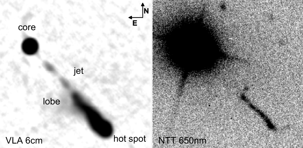
Figure 1: The quasar 3C 273 at radio (left) and optical (right) wavelengths. The main morphological features are indicated. The radio jet terminates in the bright radio hot spot at a distance of 21$\aas@@fstack{\prime\prime}$3 from the core. The faint extensions visible to the north of both ends of the optical jet are not detected at radio wavelengths.

As indicated in Figure 1, the radio jet is detected all the way from the core out to the hot spot. The faint optical structure, however, although coinciding in position angle with the line joining radio components A (hot spot) and B (core), seems to be detectable only outwards of $\approx 11$″. It also terminates about 1″ before the peak in the radio hot spot is reached. At the quasar’s redshift of 0.158 the projected length is $\approx$60 kpc. Greenstein & Schmidt (GS64 (1964)) in their detailed study of 3C 273 and 3C 48 briefly discuss also this jet. Their spectrum of its outer end exhibited a featureless blue continuum and they assumed the optical radiation is of the same origin as the radio emission, i.e. synchrotron radiation from relativistic particles. This was proven by Röser & Meisenheimer (HJRM86 (1986), HJRM91 (1991)) using optical polarimetry. Further hints about the synchrotron emission are provided by studies of the spatially resolved continua of individual knots in the jet. Meisenheimer & Heavens (MH86 (1986)) present a simple model describing the global shape of the continuum including an exponential cut-off observed in the hot spot at the jet’s outer end reflecting the maximum energy gained by the relativistic particles. Applying this model to the other knots in the jet indicates that we also see distributions of relativistic particles truncated at some maximum energy, except for the innermost visible knot (Meisenheimer et al.  MNHJR96p (1996)), which essentially has no cut-off at all. In view of these results the marginal detection of X-ray emission by Harris & Stern (HS87x (1987)) would naturally be associated with this innermost knot, although they place the centroid of the X-ray emission further out.

We have therefore used the ROSAT HRI with its better spatial resolution and sensitivity to verify the X-ray emission from this jet and to gain further insight into the emission mechanism.

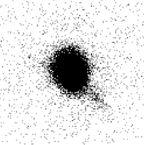
Figure 2: Unprocessed image of 3C 273 from the first observing block clearly showing the jet towards the SW.

3 ROSAT Observations

The data were collected in two observing cycles. In a 17.991 ksec integration (January 1992) we clearly detected the jet without any image processing (see Figure 2). As the signal-to-noise ratio (S/N) was not sufficient for detailed studies, 3C 273 was re-observed in December 1994/January 1995 for a total of 68.154 ksec (quoted times as “accepted” by the ROSAT standard reduction analysis).

3.1 Improving the resolution

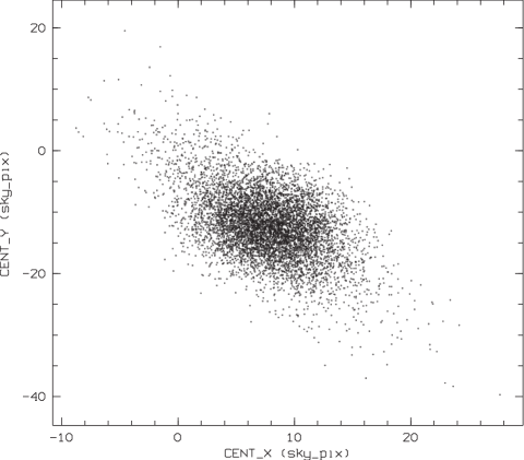
Figure 3: Centroids of the quasar photons for all 10sec intervals of observing block 2.

Images (sky pixel size 0$\aas@@fstack{\prime\prime}$5) have been produced from the event tables using the EXSAS package provided from the ROSAT group at MPE in Garching. However, the resulting point-spread function turned out to be unsatisfactory. Whereas in the call for proposals the integral point response function of the ROSAT-XTE + HRI was quoted to have a width of 5″, the FWHM of the images as produced from the raw data was typically larger than 6″. This discrepancy is due to inaccuracies in the aspect solution, which determines the sky coordinates for each photon detected. Obviously in the standard aspect solution the spacecraft wobble with a period of 402 sec is not completely corrected for (see Figure 3).

HZ 43	$\Delta$t	FWHM 1	FWHM 2	FWHM1 /	Max1 /
data set #	[sec]	[sky pixel]	[sky pixel]	FWHM2	Max2
100194	5806	7.64	15.44	0.49	1.88
141873	9142	8.40	18.53	0.45	5.57
142544	2719	9.11	18.93	0.48	4.63
142545	2569	8.81	19.34	0.46	5.48
142546	5353	9.48	20.03	0.47	5.47
142547	2275	8.67	19.17	0.45	5.50
142549	5884	9.17	19.71	0.47	5.36
142550	2608	8.62	18.56	0.46	4.59
	average	8.89	19.18
	r.m.s.	0.37	0.56
3C 273 data	85067	9.065	19.00	0.477

Table 1: Comparison of the point-spread-function for the white dwarf HZ 43 and 3C 273 in terms of two Gaussian components with widths FWHM1 and FWHM2 (see Figure 5). Units are sky pixels of 0 $\aas@@fstack{\prime\prime}$5.

With a count rate in the HRI of 2.8 cts/sec the signal from the quasar core itself is sufficiently strong to allow a shift-and-add procedure as follows: All integrations are divided into time bins of 10 sec duration and the centre of gravity of the photons from the quasar core are calculated for each interval. Photons were restricted to a raw amplitude between 2 and 8, typical for the quasar. The average accuracy of the centroid positions was 0$\aas@@fstack{\prime\prime}$64 in X and 0$\aas@@fstack{\prime\prime}$70 in Y-direction. The interval of 10 sec was a compromise between sufficient time resolution and positional accuracy. These offsets from the nominal centre position as a function of time directly correspond to the remnant pointing errors due to the insufficiently corrected wobble motion. They were interpolated in time by splines and the detected position of every photon was corrected as a function of its arrival time.

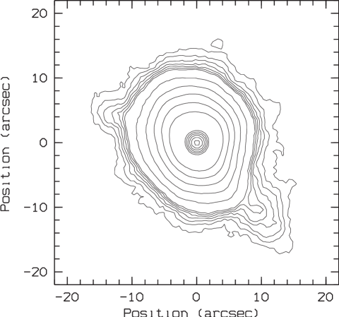
Figure 4: Isophote plot of the final image (left). Contours are at 2, 3, … 8, 16 … 1024, 1124, … 1824 counts. Note the jet to the SW and the source to the NE of the quasar. An elongation of the isophotes in the general direction of the jet is evident.

For comparison the same procedure was applied to eight data sets from the ROSAT archive for the white dwarf HZ 43, which is definitively a point source. To derive the radial image profile, each data set was sampled on concentric circles around the quasar respectively white dwarf with radii in steps of 0$\aas@@fstack{\prime\prime}$5. For each circle a constant was fitted to the data giving the azimuthally averaged intensity profile. The “core” of these profiles was decomposed by a least-square-fitting procedure into two Gaussians, neglecting the very extended exponential component discussed in the HRI calibration report (David et al. DHK99 (1999)). The shape of the point-spread-function (PSF) in the raw images changed from observation to observation. But as can be seen from Table 1 the profile of the de-jittered images was constant within the error. As indicated in Table 1 and demonstrated by Figure 5 and Figure 6, the resolution could be enhanced to 4$\aas@@fstack{\prime\prime}$5 this way. A similar procedure was described by Morse (Morse94 (1994)).

From this analysis we conclude that there is no discernable difference in the core profile between quasar and white dwarf in the averaged intensity profiles, i.e. the quasar core is unresolved at X-rays. Only in the halo the intensity of the quasar is slightly above the normalized white dwarf profile.

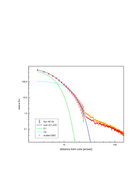
Figure 5: Radial profile of 3C 273 compared with that of the white dwarf HZ 43 (observation #141873) after re-centring of the photons (refer also to Table 1). Not the good coincidence in the inner part with the sum of two Gaussians for both objects. Error bars have been omitted beyond 24 pixels to bring out the difference bewtween white dwarf and quasar halo.

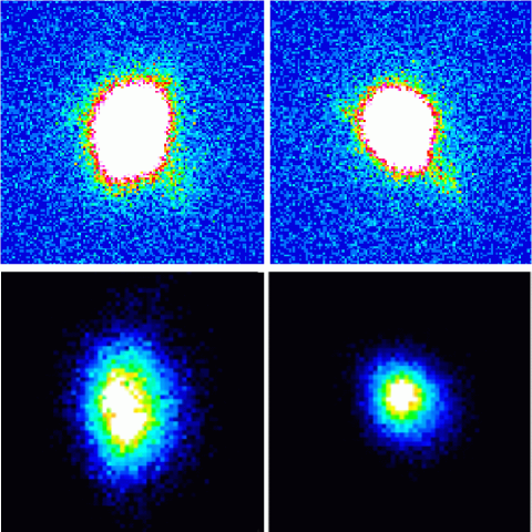
Figure 6: ROSAT HRI image of 3C 273 from the second observing block before and after re-centring the photons (top). Corresponding images of HZ 43 (#142544) are shown for comparison (bottom). The QSO images are optimised to show the jet, whereas the white dwarf images should best show the circularisation of the PSF.

3.2 Fitting the quasar’s point-spread-function

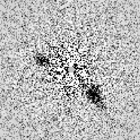
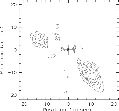
Figure 7: Background subtracted image of 3C 273. The background underneath the quasar is flat and shows the increased noise due to the intense signal subtracted. The white rectangle indicates the region over which the jet’s X-ray emission was summed up. The isophotes clearly show the extent of the X-ray emission all along the jet.

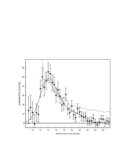
Figure 8: Trace along the jet. The thin line represents the background signal due to the quasar, summed over the same area as the jet signal. The thick line is the model fit by 5 Gaussians described in the text.

The X-ray signal from the jet of 3C 273 is very weak and is located in the wings of the complicated point-spread-function of the bright quasar core (total intensity ratio 400:1). Therefore the X-ray emission from the jet has to be isolated from this underlying point-spread-function background. Using the azimuthally averaged profiles derived above to analyse the point-spread-function is not sufficiently accurate to isolate the jet’s weak signal and measure its flux. A better model of the point-spread-function had to be obtained by fitting the signal sampled along concentric circles in four sections by polynomials of order 3, with section boundaries at 30, 120, 210 and 300^∘. In this way a satisfactory flat background also interior to the optically visible jet region is achieved (Figure 7). It should be pointed out that the result of the background modelling does strongly depend on the model parameters. With the current resolution of 4$\aas@@fstack{\prime\prime}$5 and the steep intensity gradients towards the quasar core it cannot be completely excluded that the relatively complicated model absorbs a moderately extended component in the inner part of the jet ( $r<10\arcsec$).

3.3 The X-ray signal from the jet

The count rate of the X-ray emission from the jet was derived from the PSF-subtracted image. In a window encompassing the jet we measured 644 counts. The background in several windows of the same size and at the similar distance to the quasar was measured to be $(28.6{\pm}13.5)$ counts. We therefore deduce a total jet flux of 610 counts in 85068 sec. The same procedure yields 253 counts for the object to the NE of the quasar. To convert this to a flux density we integrated a synchrotron power-law f${}_{\nu}\propto$$\nu$^α over the effective collecting area of the ROSAT HRI as a function of frequency (effective energy 1.17 keV corresponding to $2.83\times 10^{17}$ Hz) including absorption due to a neutral hydrogen column of $1.8\times 10^{20}$ cm^-2 (Otterbein Otterbein92 (1992)) using the cross-sections from Morrison & McCammon (MMcC83 (1983)) for a solar abundance. To represent synchrotron emission we used spectral indices $\alpha=-1$ and  $-2$ and thus obtained an integral flux density of $(36.6{\pm}2.8)$ and $(14.9{\pm}1.1)$ nJy for the jet and $(15.2{\pm}1.1)$ and $(6.2{\pm}0.5)$ nJy for the object in the NE of the quasar. If we assume a spectral index of $\alpha=0$ (resembling thermal bremsstrahlung) the corresponding values are $(57.1{\pm}4.3)$ nJy for the jet and $(23.7{\pm}1.8)$ nJy for the object in the NE. The error was formally derived from the scatter in the background determination.

Knot	Position [″]	Flux [nJy]
		$\alpha=-2$	$\alpha=-1$	$\alpha=0$
A	13.2	5.9	14.4	22.5
B	15.0	4.7	11.4	17.8
C	17.2	1.9	4.8	7.5
D	19.8	1.2	2.9	4.6
H	22.0	1.2	3.0	4.7
sum		$14.9{\pm}1.1$	$36.6{\pm}2.8$	$57.1{\pm}4.3$

Table 2: X-ray flux of the jet’s components in the ROSAT HRI band (at 1.17 keV corresponding to $2.83\times 10^{17}$ Hz).

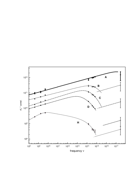
Figure 9: Spectra of the individual knots along the jet of 3C 273. The spectra of the individual knots were multiplied by constants to shift them vertically for clarity (0.5 for H, lowest spectrum, 2 for D, 20 for C, 100 for B and 380 for A, uppermost spectrum). The X-ray points at the far right cover the range found for the range in spectral index between 0 and $-2$. These points cannot be a continuation of the synchrotron spectra except possibly for knot A. The power-law meeting the X-ray point (except for knot A) indicates a hypothetical second synchrotron component with a spectral index of $-0.82$ (low frequency average over knots A to D). Such a component would not be detectable in currently observed wavebands except the X-rays.

Inspection of Figure 7 suggests that the X-ray emission from the jet is extended in the radial direction all along the visible jet. We therefore rotated the background subtracted image by 47$\aas@@fstack{\circ}$8 around the quasar core to sum the jet’s signal over the 20 pixel rows encompassing it. The resulting trace along the jet is shown in Figure 8. This run of the X-ray emission along the jet was analysed in a similar manner as the optical and radio emission (Röser & Meisenheimer HJRM91 (1991)): Gaussian profiles with constant width of 4$\aas@@fstack{\prime\prime}$5 were placed at the positions of knots A, B, C, D and H. Their peak was adjusted via a least square fit to represent the trace of X-ray emission along the jet (Table  2).

The strongest X-ray signal originates from the positions of knots A and B, much weaker emission is found further out, possibly out to the hotspot H. Due to the steeply rising quasar background, and to uncertainties in background modelling mentioned above, the onset of the jet’s X-ray emission is somewhat uncertain. On the basis of our data no X-ray emission is detected from the jet inwards of knot A.

The X-ray source to the NE of the quasar does not show any optical counterpart on our deep images, neither in the radio nor in the optical. Due to its weakness we cannot say if it is extended or not in the X-rays. Its relation to 3C 273 and its nature remain unknown.

4 Origin of the X-ray emission

To shed light onto the possible emission mechanism(s) giving rise to the jet’s X-ray emission, the above data were combined with results from our radio-to-optical studies at 1$\aas@@fstack{\prime\prime}$3 resolution (Meisenheimer et al. MYHJR97 (1997), Neumann et al. NMHJR97 (1997), Röser & Meisenheimer HJRM91 (1991)) to investigate the run of the continuum across the electromagnetic spectrum for the different regions along the jet. We plot the spectra of knots A, B, C, D, and H in Figure 9, where the flux was multiplied by different factors to disentangle the individual spectra in the graph. The continua are model spectra as described by Heavens & Meisenheimer (HM87 (1987)) and Meisenheimer & Heavens (MH86 (1986)). They result from Fermi acceleration of particles in a strong shock and include the radiation losses in a finite down-stream region. The exponential cut-off reflects the maximum energy obtained by the particles and is well established for knots B to H also by our recent HST WFPC2 data at 300 nm (Jester et al., in preparation). It is evident that in general the X-ray flux level is not a continuation of the radio-optical synchrotron cut-off continuum. Therefore different emission mechanisms have to be discussed for the individual knots.

4.1 Synchrotron radiation from the jet

Only for knot A does the extrapolation of the radio-to-optical continuum approximately meet the X-ray flux level. Extrapolation of the $\lambda$6cm flux with the low frequency spectral index of knot A ($\alpha=-0.83)$ into the ROSAT range predicts an X-ray flux of 32 nJy, only a factor of roughly two above the observed level. Whereas in Meisenheimer et al. (MNHJR96p (1996)) a lower limit to the cut-off frequency for knot A could be set at about $5\times 10^{16}$ Hz, we now have to increase this value by about a factor of 50 (see Figure 9). According to standard synchrotron theory we can therefore place a new lower limit to the maximum energy of the relativistic particles in knot A of

$$\gamma_{c}=10^{6}\times\sqrt{{{\frac{{\nu_{c}}}{{1.26\times 10^{15}{\kern 1.0pt}Hz}}}\mathord{\left/{\vphantom{{\frac{{\nu_{c}}}{{1.26\times 10^{15}{\kern 1.0pt}Hz}}}{\frac{{B_{\bot}}}{{30{\kern 1.0pt}nT}}}}}\right.\kern-1.2pt}{\frac{{B_{\bot}}}{{30{\kern 1.0pt}nT}}}}}=3\times 10^{7}$$

where we have used the minimum energy field of 67 nT. For the other knots the primary synchrotron component producing the observed radio-to-optical continuum exhibits an exponential cut-off in the optical/UV-range (Meisenheimer et al. MNHJR96p (1996)). To maintain the synchrotron scenario also for these regions a second particle population with higher maximum energy has to be invoked. These populations are indicated in Figure 9 connecting to the ROSAT HRI points with an assumed spectral index of $\alpha=-0.82$, the low-frequency average for knots A to D. The required density of relativistic particles in these hypothetical components decreases outwards along the jet. It is a factor of 5 below the density of the particles producing the observed radio-to-optical continuum for knot B and a factor of 15 and 200 below that in knot C and D, respectively. The small fraction of relativistic particles make it very hard to detect them at e.g. optical wavelengths. However, if this second population is confined to some centres of very effective acceleration on sub-arcsecond scales, we expect to see deviations from the cut-off spectrum in the optical spectral index map derived from our HST R- and U-band data at a resolution of 0$\aas@@fstack{\prime\prime}$2 (Jester et al. 2000, in preparation).

4.2 Synchrotron Self-Compton emission (SSC) from the jet

Prime sources for inverse Compton emission are compact regions with high radio photon densities in the jet, for which the hot spot H is the most likely candidate. The size of the emission region and the radio flux originating from it determine the amount of synchrotron-self-Compton emission. We have calculated the inverse Compton emission along the lines given by Blumenthal & Tucker (BT70 (1970)) as follows: The most compact component certainly is the hot spot’s acceleration region, where the optically radiating particles are produced. Its contribution to the synchrotron spectrum can be inferred from the low-frequency power-law and the high-frequency cut-off. The intermediate range with the break in the continuum (see Figure 9) is dominated by the superposition of the down-stream regions, where the relativistic particles already have lost part of their energy. Connecting the cut-off part smoothly with a power-law of index $-0.60$ we estimate the 5 GHz-flux from the acceleration region itself to be about 0.1 Jy. From the most recent analysis of the hot spot’s spectrum by Meisenheimer et al. (MYHJR97 (1997)) we infer a thickness of the emission region close to the internal shock (Mach disk) of 1.4 pc, the width perpendicular to the jet (from our best-resolved radio map) is taken to be 2.2 kpc (circular cross-section assumed). For a minimum energy field of 35 nT (assumed constant over the entire hot spot in the model) we set the density in relativistic particles in this volume to reproduce the above estimated $\lambda$6cm flux of 0.1 Jy. Integrating this synchrotron emission over the range 10 MHz to $5\times 10^{4}$ GHz (corresponding to Lorentz-factors of 100 to $2\times 10^{5}$) produces an inverse Compton flux of about 1 nJy, to within factors of 2 to 4 what is observed (see Table 2). As this is only a rough estimate to check the order of magnitude the discrepancy could well be removed by fine-tuning the parameter assumed (filling factor, geometry ).

For the other knots synchrotron-self-Compton emission fails to meet the observed level by orders of magnitude, e.g. for knot A we expect an inverse Compton X-ray flux of only 0.01 nJy. As the photon density of the microwave background radiation is one order of magnitude less than the synchrotron photon density in all knots, its photons cannot account for the X-ray flux via inverse Compton scattering either.

4.3 Thermal Bremsstrahlung from the jet

If future high resolution observations fail to reveal locations of $\nu_{c}\gg 10^{15}$ Hz in knots B, C, and D, there remains the bremsstrahlung emission from a thermal plasma as a last resort to explain the jet’s X-ray emission outside knot A and the hot spot. A plasma at 10⁸ K and with an electron density of 1 cm^-3 spread over the volume of a typical jet knot ($0\aas@@fstack{\prime\prime}5\times 0\aas@@fstack{\prime\prime}2$ from our HST images, Jester et al. 2000, in preparation) would produce an X-ray flux in the ROSAT window corresponding to 0.01 nJy. Even with this unrealistically high electron density this is orders of magnitude below the observed X-ray flux level. Furthermore any sufficiently dense thermal plasma would result in total depolarisation of the jet’s radio emission and in a substantial rotation measure. Both are not observed (Conway et al. CGPB93 (1993)). So thermal bremsstrahlung is highly unlikely to account for the observed X-ray flux.

5 The X-ray halo of 3C 273

For the comparison of the quasar’s profile with that of the white dwarf, the normalization constant had been optimised over the range 3″ to 13″, where the profiles show excellent agreement. However, it is evident from Figure 5 that the quasar profile lies systematically above the profile of the stellar source beyond radii of about 15″. Although the error of individual data points is large, we regard the systematic deviation as real and attribute it to an extended X-ray halo of the quasar (3C 273 had been observed on-axis, the pointing for HZ 43 was 1′ off-axis). To isolate the X-ray flux from this halo we have used the scaling from Figure 5 and subtracted the azimuthally averaged HZ 43-profile from the averaged quasar profile (Figure 10). This differential profile was fitted with a King profile (Jones & Forman JF84 (1984))

$$P(r)=P(0)\left[{1+\left({r/a}\right)^{2}}\right]^{-3*\beta+0.5}$$

with P(0) = 3.6, a = 10$\aas@@fstack{\prime\prime}$8 $\hat{=}$ 28.8 kpc, $\beta$ = 0.6758 determined from a least square fit to the data points between 12$\aas@@fstack{\prime\prime}$5 and 80″ from the core. Although the formal errors for these parameters are large, we nevertheless used them for our numerical estimates, as they describe the data reasonably well. The King-profile was integrated up to give the total X-ray flux from the halo of 232 nJy corresponding to a luminosity in the HRI band of $3.4\times 10^{43}$ erg/sec (spectral index $\alpha=0$ assumed). To convert this into an estimate of the physical parameters we assumed a plasma temperature of $2.7\times 10^{7}$ K as in the M 87 halo (Böhringer et al. BBSVHT94 (1994)) and that the plasma is confined with constant density to within the core radius. From these assumptions a density of $6\times 10^{4}$ H-atoms/m³ is derived for the central part of the halo. This is a factor of 10 above the upper limit derived from EINSTEIN observations by Willingale as quoted by Conway et al. (CDFR81 (1981)). The typical density of the thermal plasma in the cores of rich clusters of galaxies is a factor of 10 below this value (Jones & Forman JF84 (1984)) but the density derived above for the halo of 3C 273 matches the central density of $(7{\pm}2)\times 10^{4}$ m^-3 derived for the central density derived for the intra-cluster medium around Cygnus A (Carilli et al. CPH94 (1994)).

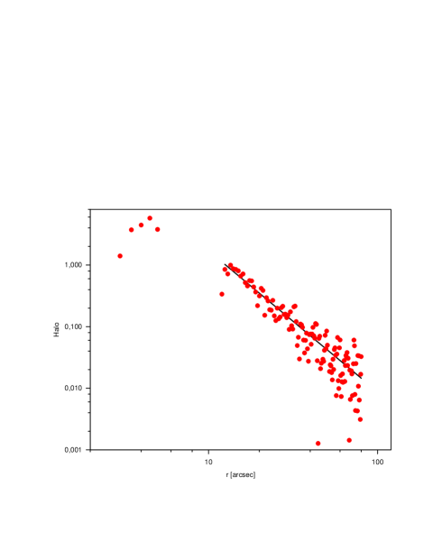
Figure 10: Azimuthally averaged radial profile of the quasar halo’s X-ray emission. The fit with a King profile is shown between 12$\aas@@fstack{\prime\prime}$5 and 80″ from the core.

6 Conclusions

ROSAT HRI observations confirm the X-ray emission from the jet of 3C 273 as suspected on the basis of the EINSTEIN HRI observations. They furthermore show that the X-rays originate from all along the jet, probably including the hot spot. While the jet’s radio emission is highly peaked towards the outer end, the optical emission is more or less constant along the jet. This trend with wavelength continues at X-rays in that these are strongly peaked now at the inner end (knots A/B).

Despite the considerably improved data base the problems with the interpretation of the jet’s X-ray emission (see Harris & Stern HS87x (1987)) still remain. Whereas the X-ray emission from the jet of M 87 might well be due to the synchrotron emission process (Neumann et al. NMHJRF97 (1997), Röser & Meisenheimer RingbergIV (1999)), the situation is less clear for the jet of 3C 273. An extrapolation of the radio-to-optical synchrotron continuum could only explain the X-ray emission from the innermost knot A, it fails for the rest of the jet. Any X-ray emission from the hot spot up to the level we found can be accounted for by synchrotron-self-Compton emission. The emission mechanism for knots B to D remains a mystery, as — except for an hypothetical high-energy synchrotron component — all three mechanisms discussed above cannot account for the X-ray emission.

The forthcoming observations of 3C 273 by CHANDRA will provide X-ray data at higher resolution and with spectral information. High spatial resolution will test if the X-ray emission does indeed coincide with the radio-optical synchrotron continuum emission, not necessarily the case for thermal bremsstrahlung emission. X-ray spectra will set important constraints on the emission mechanism mainly via the spectral slope in the X-ray band, which could directly reveal a second population of relativistic particles emitting synchrotron X-rays. Thus we can expect further insight into the mystery of X-ray emission from the jet of 3C 273 within the immediate future.

- (1) Begelman, M.C., Blandford, R.D., Rees, M.J.,: 1984, Rev. Mod. Phys. 56, 255-351
- (2) Blumenthal, G.R., Tucker, W.H.: 1970, in X-ray Astronomy. R. Giacconi, H. Gursky (ed.). Dordrecht, Kluwer: 99-153.
- (3) Böhringer, H., Briel, U.G., Schwarz, R.A., et al.: 1994, Nature 368, 828-831
- (4) Bridle, A., Perley, R.A.: 1984, Annual Review of Astronomy and Astrophysics 22, 319.
- (5) Carilli, C.L., Perley, R.A. , Harris, D.H.: 1994, Mon. Not. Roy. Astr. Soc. 270, 173
- (6) Conway, R.G., Davis, R.J., Foley, A.R., et al.: 1981, Nat 294, 540-542
- (7) Conway, R.G., Garrington, S.T., Perley, R.A., et al.: 1993, Astronomy and Astrophysics 267, 347-362
- (8) Conway, R.G. , Röser, H.-J.: 1991, in Jets in extragalactic radio sources. H.-J. Röser , K. Meisenheimer (ed.). Springer Verlag. Lecture Notes in Physics 421, 199-216.
- (9) David, L.P., Harnden, F.R., Kearns, K.E. et al.: 1999, The ROSAT High Resolution Imager (HRI) Calibration Report. Cambridge, MA 02138, Harvard-Smithsonian Center for Astrophysics.
- (10) Greenstein, J.L., Schmidt, M.: 1964, Astrophys. J. 140, 1-34
- (11) Harris, D.E., Stern, C.P.: 1987, Astrophys. J. 313, 136-140
- (12) Harris, D.E., Hjorth, J., Sadun, A.C., Silverman, J.D., Vestergaard, M.: 1999, Astophys. J. 518, 213-218
- (13) Heavens, A.F., Meisenheimer, K.: 1987, Mon. Not. Roy. Astr. Soc. 225, 335-353
- (14) Jones, C., Forman, W.: 1984, Astrophys. J. 276, 38 - 55
- (15) Leliévre, G., Nieto, J.-L., Horville, D., et al.: 1984, Astronomy and Astrophysics 138, 49-56
- (16) Meisenheimer, K., Heavens, A.F.: 1986, Nature 323, 419
- (17) Meisenheimer, K., Neumann, M., Röser, H.-J.: 1996, in Jets from Stars and Galactic Nuclei. W. Kundt (ed.). Berlin Heidelberg New York p. 230-237.
- (18) Meisenheimer, K., Yates, M.G., Röser, H.-J.: 1997, Astron. Astrophys. 325, 57-73
- (19) Morrison, R., McCammon, D.: 1983, Astrophys. J. 270, 119-122
- (20) Morse, J.A.: 1994, PASP 106, 675-682
- (21) Neumann, M., Meisenheimer, K., Röser, H.-J.: 1997, Astron. Astrophys. 326, 69-76
- (22) Neumann, M., Meisenheimer, K., Röser, H.-J., et al.: 1997, Astron. Astrophys. 318, 383-389
- (23) Otterbein, K.: 1992, Diplomarbeit Universität Tübingen
- (24) Röser, H.-J., Meisenheimer, K.: 1986, Astron. Astrophys. 154, 15-24
- (25) Röser, H.-J., Meisenheimer, K.: 1991, Astron. Astrophys. 252, 458-474
- (26) Röser, H.-J. , Meisenheimer, K., Eds.: 1993, Jets in Extragalactic Radio Sources. Lecture Notes in Physics. Berlin, Heidelberg, New York, Springer Verlag.
- (27) Röser, H.-J., Meisenheimer, K., Eds.: 1999, The Radio Galaxy Messier 87. Lecture Notes in Physics. Berlin, Heidelberg, Springer Verlag.
- (28) Röser, H.-J., Meisenheimer, K., Neumann, M., et al.: 1997, Reviews in Modern Astronomy 10, 253-261.