Abstract

We report the results on Big Bang Nucleosynthesis (BBN) based on an updated code, with accuracy of the order of $0.1\%$ on ${}^{4}He$ abundance, compared with the predictions of other recent similar analysis. We discuss the compatibility of the theoretical results, for vanishing neutrino chemical potentials, with the observational data. Bounds on the number of relativistic neutrinos and baryon abundance are obtained by a likelihood analysis. We also analyze the effect of large neutrino chemical potentials on primordial nucleosynthesis, motivated by the recent results on the Cosmic Microwave Background Radiation spectrum. The BBN exclusion plots for electron neutrino chemical potential and the effective number of relativistic neutrinos are reported. We find that the standard BBN seems to be only marginally in agreement with the recent BOOMERANG and MAXIMA-1 results, while the agreement is much better for degenerate BBN scenarios for large effective number of neutrinos, $N_{\nu}\sim 10$.

PACS number(s): 98.80.Cq; 98.80.Ft

1 Introduction

The synthesis of light nuclei in the early universe, the Big Bang Nucleosynthesis (BBN), represents one of the most striking evidence in favour of standard cosmology, and since its proposal [1], it has been extensively used as one of the best laboratories where to test cosmological models and/or elementary particle physics. The appealing feature of BBN is that, in its standard version, it relies on quite solid theoretical grounds, which makes the predictions for $D$, ${}^{3}He$, ${}^{4}He$ and ${}^{7}Li$ abundances, whose primordial values are only partially modified by the subsequent stellar activity, quite robust.

Recently, the experimental accuracy in measurements of the light primordial nuclide abundances, mainly ${}^{4}He$, has been highly improved, reaching a precision of the order of $1\%$. Similar improvements have been also obtained for both Deuterium ($D$) and ${}^{7}Li$ relative abundances, $Y_{D}\equiv D/H$ and $Y_{{}^{7}Li}\equiv~{}^{7}Li/H$, but, unfortunately, the refinement of the experimental techniques does not yet correspond to a clear picture of the primordial nuclide densities. This is mainly due to an uncomplete understanding of systematic errors. In particular, measuring the primordial ${}^{4}He$ mass fraction, $Y_{p}$, from regression to zero metallicity in Blue Compact Galaxies, two independent surveys obtained two results, a low value [2],

$$Y_{p}^{(l)}=0.234{\pm}0.003~{}~{}~{},$$ (1.1)

and a sensibly larger one [3],

$$Y_{p}^{(h)}=0.244{\pm}0.002~{}~{}~{},$$ (1.2)

which are compatible at $2\sigma$ level only.

As in a recent analysis [4], we here adopt a more conservative value, with a larger error (hereafter we always use 1$\sigma$ errors)

$$Y_{p}=0.238{\pm}0.005~{}~{}~{}.$$ (1.3)

A similar dichotomy holds in $D$ measurements as well, where the study of distant Quasars Absorption line Systems (QAS), is thought to represent a reliable way to estimate the primordial Deuterium. In this case, observations in different QAS leads to the incompatible results [5, 6, 4]

$$Y_{D}^{(l)} = \left(3.4{\pm}0.3\right)10^{-5}~{}~{}~{},$$ (1.4)

$$Y_{D}^{(h)} = \left(2.0{\pm}0.5\right)10^{-4}~{}~{}~{}.$$ (1.5)

Finally, a reliable estimate for ${}^{7}Li$ primordial abundance is provided by the Spite plateau, observed in the halo of POP II stars [7, 8]. The observations give the primordial abundance [9],

$$Y_{{}^{7}Li}=\left(1.73{\pm}0.21\right)10^{-10}~{}~{}~{}.$$ (1.6)

From the theoretical point of view, the BBN predictions are obtained by numerically solving a set of coupled Boltzmann equations, which trace the abundances of the different nuclides in the framework of standard Big Bang cosmology [10]. The collisional integrals of the above equations contain all $n\leftrightarrow p$ weak reaction rates and a large nuclear reaction network [11].

The increasing precision in measuring the primordial abundance has recently pushed the theoretical community to make an effort to develop new generation BBN codes [12, 13], with a comparable level of accuracy. In a recent series of papers, in the framework of the standard cosmological model, the present authors [14] and other groups [12] have performed a comprehensive and accurate analysis of all the physical effects which influence ${}^{4}He$ mass fraction up to $0.1\%$.

Since almost all neutrons present at the onset of nucleosynthesis are fixed into ${}^{4}He$, its abundance is mainly function of the neutron versus proton abundances, at the time of $n\leftrightarrow p$ weak interactions freeze out, which takes place for $T\sim 1\,MeV$. To improve the accuracy on the ${}^{4}He$ prediction it is demanding to reach an accuracy level of the order of $1\%$ in the estimate of the $n\leftrightarrow p$ rates, well beyond the simple Born approximation. This has been performed by considering a number of additional contributions, which, ordered according to their relative weight, are the following:
i) electromagnetic radiative and Coulomb corrections [15, 16];
ii) finite nucleon mass corrections [17, 14];
iii) thermal radiative effects induced by the presence of a surrounding plasma of $e^{\pm}$ and $\gamma$ [18, 14];
iv) corrections to the equation of state of the $e^{\pm},\,\gamma$ plasma due to thermal mass renormalization [19, 12, 13];
v) the residual neutrino coupling to the plasma during $e^{+}e^{-}$ annihilation, affecting the neutrino to photon temperature ratio [20, 12, 13].

Unfortunately, a similar systematic analysis of all corrections up to the desired level of accuracy cannot be performed for the other input parameters of the theory. The theoretical estimates do depend in fact on the values of the neutron lifetime, as well as on several nuclear reaction cross sections, which are poorly known in the energy range relevant for BBN. This introduces a certain level of uncertainty on the light element abundances. This aspect has been studied in two different approaches, either using Monte Carlo methods [21] to sample the error distributions of the relevant reaction cross sections, or, alternatively, using a linear error propagation [22], with comparable results.

In this paper, we further refine our previous predictions by using a new version of our numerical code, where the full dependence of the BBN equations on the electron chemical potential is accurately implemented. Furthermore, for the standard scenario (vanishing neutrino chemical potentials) we perform an accurate likelihood analysis in the space of the two free parameters of the model, the effective number of neutrinos, $N_{\nu}$, and the baryon to photon ratio $\eta$.

While the value of electron chemical potential is bounded, by neutrality, by the value of $\eta$, this is not the case for neutrino–antineutrino asymmetries which, in principle, can be quite large. The influence of the neutrino chemical potentials on BBN predictions (degenerate BBN) has been considered in the past [23]. One relevant aspect of this analysis, which is worth stressing, is that degenerate BBN allows for a better agreement with observations at values of $\eta$ larger than, say, $6{\cdot}10^{-10}$, while standard BBN prefers smaller values, $\eta\sim(2\div 6){\cdot}10^{-10}$. We will discuss this in detail in the paper. This feature is particularly relevant in view of the recent analysis of the BOOMERANG and MAXIMA-1 results [24] on the acoustic peak of the Cosmic Microwave Background Radiation (CMBR), which seems to favour a value for the baryonic asymmetry $\eta$ of the order of $10^{-9}$, larger, as we said, than what expected in the framework of standard BBN. This discrepancy may be looked as a signal in favour of a large neutrino–antineutrino asymmetry. It seems therefore demanding to re–analyze the degenerate scenario, making profit of the now available more precise BBN codes. We have performed this study, and the main result is that degenerate BBN and CMBR data seems to be compatible for large values of the effective number of neutrinos, $N_{\nu}\geq 10$ and $\eta\leq 10^{-9}$.

The paper is organized as follows. In section 2 we briefly describe the BBN set of differential equations, recast in a suitable form for a numerical solution. The light element abundances obtained from our code, for standard BBN, are then presented in section 3 as a functions of $\tau_{n}$, $N_{\nu}$ and $\eta$. Section 4 is devoted to degenerate BBN and to the bounds on neutrino chemical potentials coming from nucleosynthesis and CMBR data. Finally, in section 4, we give our conclusions.

2 The BBN set of equations

Consider $N_{nuc}$ species of nuclides, whose number densities, $n_{i}$, are normalized with respect to the total number density of baryons, $n_{B}$,

$$X_{i}=\frac{n_{i}}{n_{B}}\quad\quad\quad i=1,..,N_{nuc}~{}~{}~{}.$$ (2.1)

Alternatively, we will also make use in the following of the notation:

$$X_{1}=X_{n}~{}~{}~{}, ~{}~{}~{}~{}~{}X_{2}=X_{p}=X_{H}~{}~{}~{}, ~{}~{}~{}~{}~{}X_{3}=X_{D}~{}~{}~{},~{}~{}~{}~{}~{}$$

$$X_{5}=X_{{}^{3}He}~{}~{}~{}, ~{}~{}~{}~{}~{}X_{6}=X_{{}^{4}He}~{}~{}~{}, ~{}~{}~{}~{}~{}X_{8}=X_{{}^{7}Li}~{}~{}~{}.$$ (2.2)

The set of differential equations ruling primordial nucleosynthesis is given by [1, 13]:

$$\frac{\dot{R}}{R} = H=\sqrt{\frac{8\,\pi}{3\,M_{P}^{2}}~{}\rho_{T}}~{}~{}~{},$$ (2.3)

$$\frac{\dot{n}_{B}}{n_{B}} = -\,3\,H~{}~{}~{},$$ (2.4)

$$\dot{\rho_{T}} = -\,3\,H~{}(\rho_{T}+{\rm p}_{T})~{}~{}~{},$$ (2.5)

$$\dot{X}_{i} = \sum_{j,k,l}\,N_{i}\left(\Gamma_{kl\rightarrow ij}\,\frac{X_{l}^{N_{l}}\,X_{k}^{N_{k}}}{N_{l}!\,N_{k}!}\;-\;\Gamma_{ij\rightarrow kl}\,\frac{X_{i}^{N_{i}}\,X_{j}^{N_{j}}}{N_{i}!\,N_{j}!}\right)\equiv\Gamma_{i}(X_{j})~{}~{}~{},$$ (2.6)

$$L(\frac{m_{e}}{T},{\phi_{e}}) = \frac{n_{B}}{T^{3}}~{}\sum_{j}Z_{j}\,X_{j}~{}~{}~{},$$ (2.7)

where $\rho_{T}$ and ${\rm p}_{T}$ denote the total energy density and pressure, respectively,

$$\rho_{T} = \rho_{\gamma}+\rho_{e}+\rho_{\nu}+\rho_{B}\equiv\rho_{NB}+\rho_{B}~{}~{}~{},$$ (2.8)

$${\rm p}_{T} = {\rm p}_{\gamma}+{\rm p}_{e}+{\rm p}_{\nu}+{\rm p}_{B}~{}~{}~{},$$ (2.9)

$i,j,k,l=(1,..,N_{nuc})$, $Z_{i}$ is the charge number of the $i-$th nuclide, and the function $L(z,y)$ is defined as

$$L(z,y)\equiv\frac{1}{\pi^{2}}\int_{z}^{\infty}dx~{}x\,\sqrt{x^{2}-z^{2}}~{}\left(\frac{1}{e^{x-y}+1}-\frac{1}{e^{x+y}+1}\right)~{}~{}~{}.$$ (2.10)

Eq.(2.3) is the definition of the Hubble parameter, $H$, whereas Eq.s (2.4) and (2.5) state the total baryon number and entropy conservation in the comoving volume, respectively. The set of $N_{nuc}$ Boltzmann equations (2.6) describe the density evolution of each nuclide specie, and finally Eq.(2.7) states the universe charge neutrality in terms of the electron chemical potential, $\phi_{e}\equiv\mu_{e}/T$, with $T$ the temperature of $e^{\pm},\gamma$ plasma. Note that the neutrino energy density and pressure are included in Eq. (2.5) only for $T\geq T_{D}$.

In a previous analysis, [13], we neglected the contribution of ${\phi_{e}}$ in the BBN equations, since its effect results to be very small. In this way we obtained a substantial simplification of the set of equations (2.3)-(2.7), since the unknown functions can be reduced in this case to the $N_{nuc}+1$ ($\hat{h}\equiv n_{B}/T^{3},~{}X_{j}$). We do here release this assumption and report the results of an improved code where we take into complete account the electron chemical potential evolution. We will see, however, that all changes on the final abundances are of minor impact. In order to obtain the new equations, we note that it is more convenient to follow the evolution of the $N_{nuc}+1$ unknown functions $({\phi_{e}},~{}X_{j})$ in terms of the dimensionless variable $z=m_{e}/T$, and to use Eq. (2.7) to get $n_{B}$ as a function of ${\phi_{e}}$. The new set of differential equations may be cast in the form

$$\frac{d{\phi_{e}}}{dz}\,=\,\frac{1}{z}~{}\frac{L~{}E~{}F+(z\,L_{z}-3\,L)~{}G}{L~{}E~{}\frac{\displaystyle\delta\hat{\rho}_{e}}{\displaystyle\delta{\phi_{e}}}-L_{\phi_{e}}~{}G}~{}~{}~{},$$ (2.11)

$$\frac{dX_{i}}{dz}\,=\,-\frac{\widehat{\Gamma}_{i}}{z}~{}\frac{L_{\phi_{e}}~{}F+(z\,L_{z}-3\,L)~{}\frac{\displaystyle\delta\hat{\rho}_{e}}{\displaystyle\delta{\phi_{e}}}}{L~{}E~{}\frac{\displaystyle\delta\hat{\rho}_{e}}{\displaystyle\delta{\phi_{e}}}-L_{\phi_{e}}~{}G}~{}~{}~{},$$ (2.12)

where the functions $E$, $F$ and $G$ are given by

$$E(z,\,{\phi_{e}},\,X_{j}) = 3\,\widehat{H}-\frac{\displaystyle\sum_{i}~{}Z_{i}\,\widehat{\Gamma}_{i}}{\displaystyle\sum_{j}~{}Z_{j}\,X_{j}}~{}~{}~{},$$ (2.13)

$$F(z,\,{\phi_{e}},\,X_{j}) = 4\,\hat{\rho}_{NB}+\frac{3}{2}~{}\hat{\rm p}_{B}-z\,\frac{\delta\hat{\rho}_{e}}{\delta z}~{}~{}~{},$$ (2.14)

$$G(z,\,{\phi_{e}},\,X_{j}) = 3\,\widehat{H}~{}(\hat{\rho}_{NB}+\hat{\rm p})+\frac{z\,L}{\sum_{j}Z_{j}\,X_{j}}~{}\sum_{i}\left(\Delta\widehat{M}_{i}+\frac{3}{2\,z}\right)~{}\widehat{\Gamma}_{i}~{}~{}~{},$$ (2.15)

and $H\equiv m_{e}\,\widehat{H}$, $n_{B}\equiv m_{e}^{3}~{}\hat{n}_{B}$, $\Gamma_{i}\equiv m_{e}\,\widehat{\Gamma}_{i}$, $\rho_{T}\equiv T^{4}\,\hat{\rho}_{T}$, ${\rm p}_{T}\equiv T^{4}\,\hat{\rm p}_{T}$. Note that by using Eq. (2.7) and the previous definitions, it is possible to express $\hat{\rho}_{B}$ and $\hat{\rm p}_{B}$ as functions of $z$, ${\phi_{e}}$, and $X_{i}$ only

$$\hat{\rho}_{B} = \frac{z\,L(z,{\phi_{e}})}{\sum_{j}Z_{j}\,X_{j}}~{}\left[\widehat{M}_{u}+\sum_{j}\left(\Delta\widehat{M}_{j}\,+\,\frac{3}{2\,z}\right)\,X_{j}\right]~{}~{}~{},$$ (2.16)

$$\hat{\rm p}_{B} = \frac{L(z,{\phi_{e}})}{\sum_{j}Z_{j}\,X_{j}}~{}\sum_{j}X_{j}~{}~{}~{}.$$ (2.17)

With $\Delta\widehat{M}_{i}$ and $\widehat{M}_{u}$ we denote the i-th nuclide mass excess and the atomic mass unit, respectively, normalized to $m_{e}$. In Appendix A we report the partial derivative of $L$ with respect to $z$ and ${\phi_{e}}$, denoted with $L_{z}$ and $L_{{\phi_{e}}}$, and the quantities $\hat{\rho}_{e}$, $\delta\hat{\rho}_{e}/\delta z$ and $\delta\hat{\rho}_{e}/\delta{\phi_{e}}$ in a form which is suitable for a BBN code implementation.

Eq.s (2.11)-(2.12) are solved by imposing the following initial conditions at $z_{in}=m_{e}/(10\,MeV)$:

$${\phi_{e}}(z_{in}) = {\phi_{e}}^{0}~{}~{}~{},$$ (2.18)

$$X_{n}(z_{in}) = \left(\exp\{\hat{q}\,z_{in}\}+1\right)^{-1}~{}~{}~{},\quad\quad X_{p}(z_{in})=\left(\exp\{-\hat{q}\,z_{in}\}+1\right)^{-1}~{}~{}~{},$$ (2.19)

$$X_{i}(z_{in}) = \frac{g_{i}}{2}~{}\left(\zeta(3)\sqrt{\frac{8}{\pi}}\right)^{A_{i}-1}~{}A_{i}^{\frac{3}{2}}\,\left(\frac{m_{e}}{M_{N}z_{in}}\right)^{\frac{3}{2}(A_{i}-1)}\eta^{A_{i}-1}\,X_{p}^{Z_{i}}\,X_{n}^{A_{i}-Z_{i}}$$ (2.20)

$${\times} \exp\left\{\hat{B}_{i}\,z_{in}\right\}\quad\quad\quad\quad\quad\quad\quad\quad\quad\quad\mbox{with}~{}i=3,..,N_{nuc}~{}~{}~{}.$$

In the previous equations $\hat{q}=(M_{n}-M_{p})/m_{e}$, and the quantities $A_{i}$ and $\hat{B}_{i}$ denote the atomic number and the binding energy of the $i-$th nuclide normalized to electron mass, respectively. Finally $\eta$ is, as usual, the baryon to photon number density ratio, and ${\phi_{e}}^{0}$ the solution of the implicit equation

$$L(z_{in},\,{\phi_{e}}^{0})=\frac{11}{4}~{}\frac{2\,\zeta(3)}{\pi^{2}}~{}\eta~{}\sum_{i}Z_{i}\,X_{i}(z_{in})~{}~{}~{}.$$ (2.21)

The method of resolution of the BBN equations (2.11)-(2.12) is the same applied in [13]. It is the Backward Differentiation Formulas with Newton’s method, implemented in a NAG routine with adaptive step-size (see [13] for more details). We used the reduced network of nuclear reactions, made of 25 reactions involving 9 nuclides, since the use of the complete network affects the abundances for no more than $0.01~{}\%$.

3 Primordial abundances for standard BBN

The new BBN code has been used to produce the primordial abundances, in the standard scenario, for different values of the input parameters, namely the neutron lifetime $\tau_{n}$, the effective number of neutrinos $N_{\nu}$, defined as

$$\rho_{\nu}=N_{\nu}\,\frac{7}{4}\,\frac{\pi^{2}}{30}\,T_{\nu}^{4}~{}~{}~{},$$ (3.1)

with $\rho_{\nu}$ the total neutrino energy densities, and the final baryon to photon number density ratio $\eta$.

We consider the abundances relative to hydrogen for $D$, ${}^{3}He$, and ${}^{7}Li$,

$$Y_{D}=\frac{X_{D}}{X_{H}}~{}~{}~{},~{}~{}~{}~{}~{}Y_{{}^{3}He}=\frac{X_{{}^{3}He}}{X_{H}}~{}~{}~{},~{}~{}~{}~{}~{}Y_{{}^{7}Li}=\frac{X_{{}^{7}Li}}{X_{H}}~{}~{}~{}.$$ (3.2)

In the case of ${}^{4}He$, the quantity usually defined as mass fraction,

$$Y_{p}=\frac{A_{{}^{4}He}~{}X_{{}^{4}He}}{\sum_{j}A_{j}~{}X_{j}}~{}~{}~{},$$ (3.3)

is rather the baryon number fraction, since $A_{{}^{4}He}=4$. Note that expression (3.3) does not correspond to the true mass fraction, obviously defined as

$$Y_{p}^{m}=\frac{M_{{}^{4}He}~{}X_{{}^{4}He}}{\sum_{j}M_{j}~{}X_{j}}~{}~{}~{}.$$ (3.4)

The difference between $Y_{p}$ and $Y_{p}^{m}$ are of the order of $1\%$ and thus relevant for an accurate analysis like the one presented here. Since it is customary to express the experimental value in terms of $Y_{p}$, see (1.3), we will consider this quantity for a comparison with experimental data.

Table 1 shows the results obtained for $N_{\nu}=3$, $\tau_{n}=886.7\,s$, and $\eta=5{\cdot}10^{-10}$, compared with our previous results [13]. As one can see, the inclusion of the complete evolution of ${\phi_{e}}$ modifies the final ${}^{4}He$ abundances for less than $0.1\%$ and for few percent the other nuclides.

	$Y_{D}$	$Y_{{}^{3}He}$	$Y_{p}$	$Y_{p}^{m}$	$Y_{{}^{7}Li}$
present	$0.3609{\cdot}10^{-4}$	$0.1166{\cdot}10^{-4}$	0.2461	0.2448	$0.2879{\cdot}10^{-9}$
analysis
previous	$0.3638{\cdot}10^{-4}$	$0.1175{\cdot}10^{-4}$	0.2460	0.2447	$0.2814{\cdot}10^{-9}$
analysis

Table 1: The predictions on light element abundances obtained with the new BBN code, compared with our previous results [13].

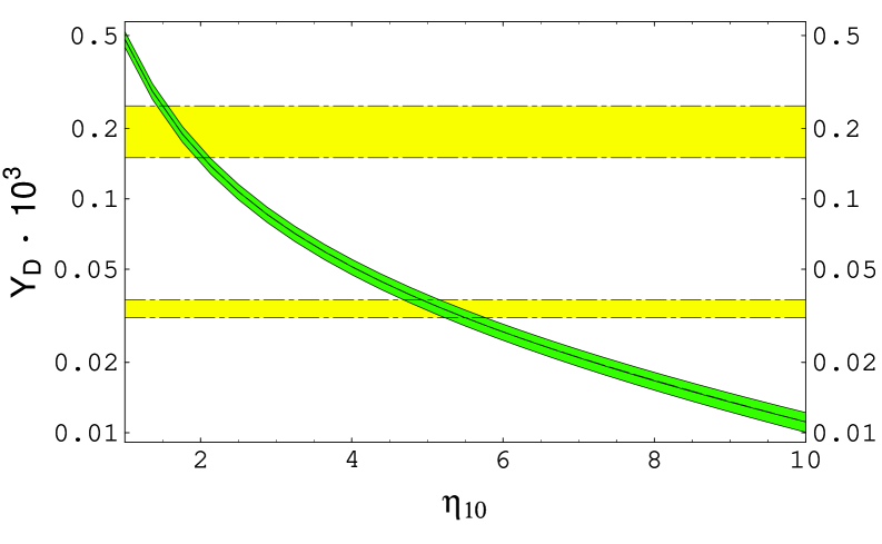
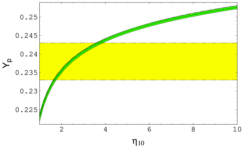
In Figures 1, 3, 5, 7 we show the theoretical predictions for the abundances (3.2)-(3.3), compared with the experimental values. Figures 2, 4, 6, 8 show the comparison between our results and the ones of Ref.s [22, 12]. The relative differences among our predictions and the results of Ref.s [22, 12] for ${}^{4}He$, in the relevant range for $\eta_{10}\equiv 10^{10}\eta$, are less than $0.25\%$, and thus probably due to different ways of taking into account subdominant effects (thermal radiative corrections). The differences are not much larger for Deuterium, but reach few percents for ${}^{3}He$ and ${}^{7}Li$, which however have very large theoretical errors due to the uncertainties on nuclear reaction rates. Note that for $D$, ${}^{3}He$ and ${}^{7}Li$ only the results of [22] are available.

$k_{i}\,{\cdot}\,Y_{i}$	$j$	$a_{j}$	$b_{j}$	$c_{j}$	$d_{j}$	$e_{j}$
$10^{3}{\cdot}D$	0	0.48212	-	0.076014	0.0015595	-
	1	0.12998	-	0.011704	0.0015438	-4.0240
	2	0.24279	-	-0.056835	-0.010037	-1.1394
	3	-0.91776	-	0.0045225	-0.014180	4.7712
	4	2.2660	-	0.27257	0.090586	-9.7616
	5	-1.1308	-	-0.20773	-0.15266	9.5377
	6	-1.4315	-	-0.096193	0.11416	-3.5489
	7	1.0751	-	0.10664	-0.031562	-
$10^{5}{\cdot}~{}^{3}He$	0	3.3201	-	0.18342	-0.0067466	-
	1	-8.8146	-	-0.60698	0.013121	0.93721
	2	7.3100	-	1.0607	-0.042731	2.1792
	3	14.543	-	-0.52115	0.26524	-5.6965
	4	-51.298	-	-1.9291	-0.72719	5.8729
	5	76.092	-	4.5046	0.94031	-8.2579
	6	-59.309	-	-3.8725	-0.58402	3.8572
	7	20.591	-	1.2760	0.13864	-
$10{\cdot}~{}^{4}He$	0	2.2289	0.0020479	0.13021	-0.0096485	-
	1	-0.052824	-0.00064726	0.0075762	0.0018598	0.27365
	2	0.59320	0.0033813	-0.013789	-0.0030398	-0.58807
	3	0.49399	-0.014272	0.082061	-0.011842	0.22190
	4	1.9579	0.041398	0.10938	0.027656	-1.3763
	5	-0.89742	-0.057323	-0.12581	-0.051066	0.93037
	6	0.34269	0.040258	0.096350	0.039127	-0.17224
	7	0.47527	-0.010753	-0.0018617	-0.013441	-
$10{\cdot}~{}^{4}He_{m}$	0	2.2184	0.0020421	0.13003	-0.0095937	-
	1	-0.44715	-0.0011625	-0.016604	0.0040428	0.44707
	2	0.94939	0.0065040	0.010744	-0.013907	-0.69814
	3	6.8365	-0.026617	0.43785	0.018033	-2.8141
	4	-1.1513	0.094984	0.0086552	-0.12409	-0.80120
	5	2.0116	-0.14739	-0.17116	0.19005	3.0861
	6	3.1081	0.11736	0.48418	-0.16606	-1.1642
	7	4.0381	-0.031739	0.088568	0.031865	-
$10^{9}{\cdot}~{}^{7}Li$	0	0.52920	-	0.15387	0.011486	-
	1	-1.5617	-	-0.42097	-0.0075472	-2.0190
	2	2.0002	-	-0.23058	-0.21878	-1.2259
	3	0.58298	-	2.9150	0.94226	9.8088
	4	-8.3304	-	-6.7141	-1.7403	-9.7328
	5	22.627	-	6.2727	1.8244	3.1404
	6	-21.053	-	-1.9273	-1.1338	0.15166
	7	6.1684	-	-0.090045	0.32046	-

Table 2: Values of the coefficients of Eq. (3.5) for light element abundances.

We have performed a fit of the previous abundances as functions of $N_{\nu}$, $\tau_{n}$, and $x\equiv\log_{10}\eta_{10}$, with an accuracy which is better than $1\%$ in the all ranges $0.5\leq N_{\nu}\leq 6$, $882.9\,s\leq\tau_{n}\leq 890.5\,s$, $0\leq x\leq 1$. In particular, for $N_{\nu}=3$ and ${}^{4}He$, our fit is accurate at $0.01\%$. The fitting functions have been chosen as

$$k_{i}\,{\cdot}\,Y_{i}\,(N_{\nu},~{}\tau_{n},~{}x) = \left[~{}\sum_{j=0}^{8}a_{j}\,x^{j}+\left(\,\sum_{j=0}^{8}b_{j}\,x^{j}\,\right)\,(\tau_{n}-\tau^{ex}_{n})+\left(\,\sum_{j=0}^{8}c_{j}\,x^{j}\,\right)\,(N_{\nu}-3)~{}+\right.$$ (3.5)

$$\left(\,\sum_{j=0}^{8}d_{j}\,x^{j}\,\right)\,(N_{\nu}-3)^{2}~{}\biggr{]}\exp\left\{~{}\sum_{j=1}^{6}e_{j}\,x^{j}~{}\right\}~{}~{}~{},$$

with all coefficients given in Table 2.

By using these expressions (3.5), as the theoretical predictions for the light element abundances, and their experimental measurements (1.3), (1.4), (1.5), (1.6) it is possible to test the compatibility of standard BBN scenario in the $N_{\nu}$–$\eta_{10}$ plane. To this end, we define a total likelihood function as

$${\cal L}(N_{\nu},\,\eta_{10})=L_{D}(N_{\nu},\,\eta_{10})~{}L_{{}^{4}He}(N_{\nu},\,\eta_{10})~{}L_{{}^{7}Li}(N_{\nu},\,\eta_{10})~{}~{}~{},$$ (3.6)

where the likelihood function for each abundance, assuming Gaussian distribution for the errors, is given by the overlap

$$L_{i}(N_{\nu},\,\eta_{10})=$$ (3.7)

$$\!\!\!\!\!\!\!\!\!\!\!=\displaystyle\frac{1}{2\,\pi\,\sigma_{i}^{th}(N_{\nu},\,\eta_{10})\,\sigma_{i}^{ex}} \int dY~{}\exp\left\{-\frac{(Y-Y_{i}^{th}(N_{\nu},\,\eta_{10}))^{2}}{2\,\sigma_{i}^{th\,2}(N_{\nu},\,\eta_{10})}\right\}\exp\left\{-\frac{(Y-Y_{i}^{ex})^{2}}{2\,\sigma_{i}^{ex\,2}}\right\}$$

In order to evaluate $L_{i}(N_{\nu},\,\eta_{10})$ we need the theoretical uncertainties $\sigma_{i}^{th}(N_{\nu},\,\eta_{10})$. In Ref. [22] a new, alternative approach to the standard Monte Carlo technique [21] has been proposed. This method is based on linear error propagation for the estimate of theoretical uncertainties on primordial abundances due to the poor knowledge of nuclear reaction rates. The light element abundances, $Y_{i}$, and the logarithmic derivatives of $Y_{i}$ with respect to the nuclear rates, $\lambda_{ik}$, are given as polynomial fits, while the variation of the abundances for a change $\delta R_{k}$ in the rate $R_{k}$ is obtained as

$$\delta Y_{i}=Y_{i}~{}\sum_{k}~{}\lambda_{ik}\,\frac{\delta R_{k}}{R_{k}}~{}~{}~{}.$$ (3.8)

Taking into account the error correlation, the error matrix results

$$\sigma_{ij}^{2}=Y_{i}~{}Y_{j}~{}\sum_{k}~{}\lambda_{ik}\,\lambda_{jk}\,\left(\frac{\Delta R_{k}}{R_{k}}\right)^{2}~{}~{}~{},$$ (3.9)

where $\Delta R_{k}$ are the $1\sigma$ uncertainties. In particular the theoretical $1\sigma$ uncertainties are given by the square root of the diagonal elements,

$$\sigma_{i}^{th}=\sqrt{\sigma_{ii}^{2}}~{}~{}~{}.$$ (3.10)

We used the Fortran code provided by the authors [26] to calculate the theoretical uncertainties $\sigma_{i}^{th}(N_{\nu},\,\eta_{10})$, which we used in Eq. (3.7).

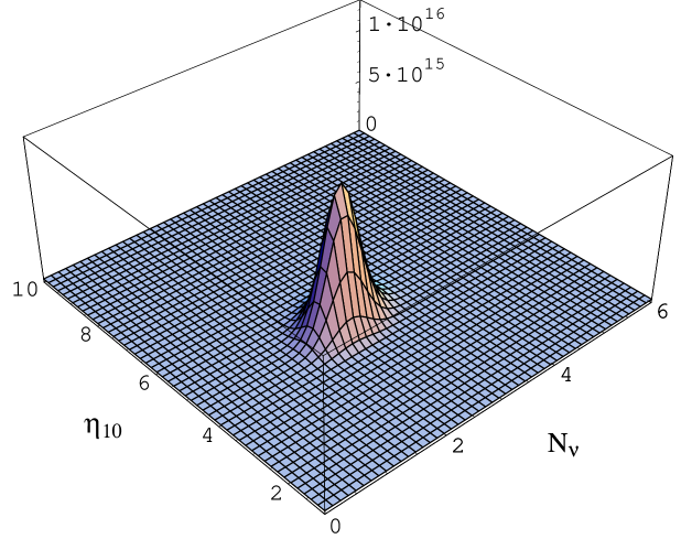
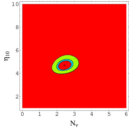
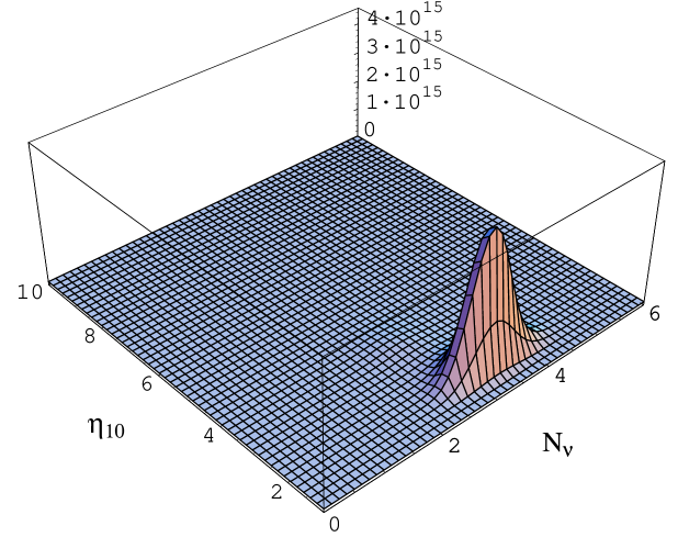
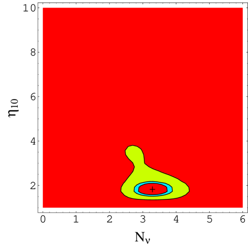
The total likelihood function (3.6) and the corresponding contour plots for $50\%$, $68\%$ and $95\%$ CL, for low and high $D$ are shown in Figures 9, 10 and 11, 12, respectively. As already clear from Figure 1, the two different experimental estimates of $D$ single out different regions for $\eta_{10}$. From the $95\%$ CL contour of Figure 10, for low $D$ we have $4.0\leq\eta_{10}\leq 5.7$, which is in fair agreement with the similar results of Ref. [4], whereas for high $D$ from Figure 12 we get $1.4\leq\eta_{10}\leq 3.7$.

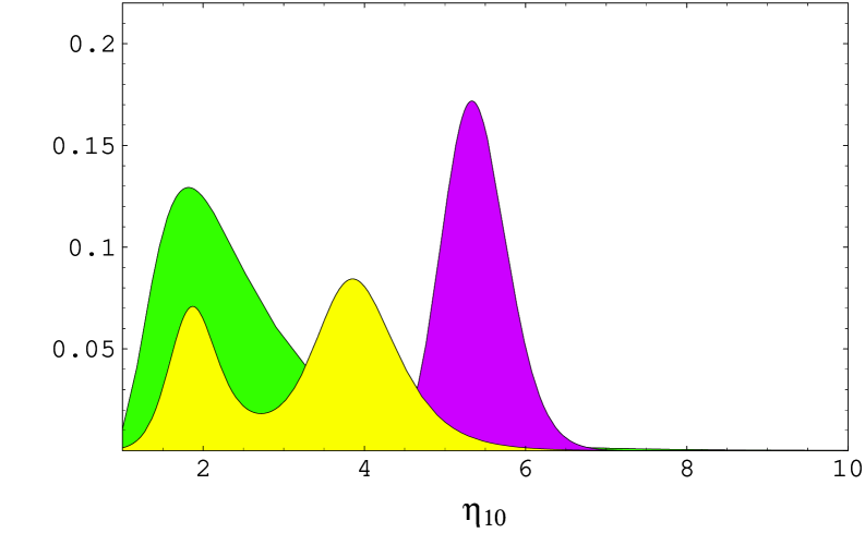
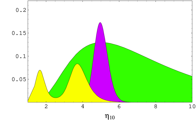
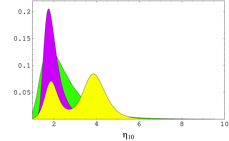
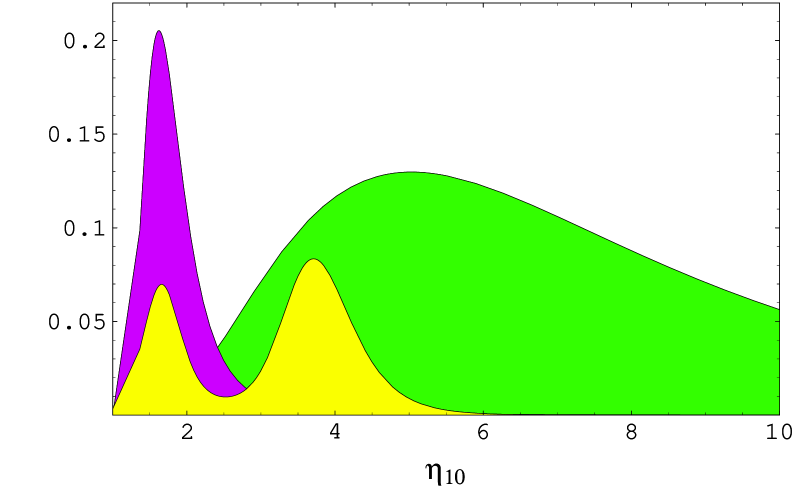
As far as $N_{\nu}$ is concerned, for low $D$ and for $95\%$ CL one has $1.7\leq N_{\nu}\leq 3.3$, whereas for high $D$ one gets $2.3\leq N_{\nu}\leq 4.4$. In both cases we obtain comparable ranges for $N_{\nu}$ with respect to Ref. [4]. The total likelihood function is peaked around the points shown as the crosses in Figures 10 and 12, which correspond to $N_{\nu}=2.44$ and $\eta_{10}=4.69$ for low $D$, and to $N_{\nu}=3.29$ and $\eta_{10}=1.81$ for high $D$. The position of the two maxima is easily understood. The Deuterium abundance is a decreasing function of $\eta_{10}$. Since lowering $\eta_{10}$ results in a smaller ${}^{4}He$ mass fraction $Y_{p}$, it is necessary to compensate this effect by increasing the universe expansion rate via a larger $N_{\nu}$. This in fact leads to a larger value for the freeze–out temperature for nucleon weak interactions and thus gives a larger amount of the initial neutron to proton density ratio. The single contributions (3.7) to the total likelihood (3.6) can be easily recognized by looking at Figures 13-16, where we show the $D$, ${}^{4}He$ and ${}^{7}Li$ likelihood functions, for both high and low Deuterium results, for the two preferred values $N_{\nu}=2.44$ and $N_{\nu}=3.29$. For the low $D$ case, a better overlap between the maxima of the single likelihoods of $D$ and ${}^{4}He$ is realized for $N_{\nu}=2.44$. The opposite situation occurs for high $D$ where to $N_{\nu}=3.29$ corresponds a better overlap of the single likelihoods.

4 BBN predictions for degenerate neutrinos

The assumption of vanishing neutrino chemical potentials can be only justified by the sake of simplicity or by the theoretical prejudice that their order of magnitude should be set by the ones of the corresponding charged leptonic partner. However, physical scenarios in which large lepton asymmetries are produced, which do not lead to a large baryon asymmetry, have been proposed in literature [27, 28, 29, 30]. They are based on the Affleck-Dine mechanism [27] or on active–sterile neutrino oscillations [31, 32]. In particular, the expected asymmetry may be different for each neutrino family. For these reasons, at least in principle, it is worth-while considering the primordial nucleosynthesis in presence of large neutrino asymmetries, i.e. for non-vanishing neutrino chemical potentials. It seems to us that this topic, which has been extensively studied in past [23], receives a renewed interest in view of the recent BOOMERANG and MAXIMA-1 results [24] on the acoustic peaks of the CMBR, which suggests a larger value of the baryonic matter contribution to the total energy density $\Omega$. In their analysis of the data they find a baryon density $\Omega_{b}h^{2}\sim 0.02\div 0.03$, or $\eta\sim(6\div 10)10^{-10}$, which, as is clear from the considerations of the previous section, is incompatible at $95\%$ CL with the standard BBN result (see Figures 10 and 12). Actually even larger values for $\Omega_{b}h^{2}$ are obtained if no constraints are imposed in the likelihood analysis (see [24]). It is the aim of this section to discuss whether a finite neutrino chemical potential may reconcile BBN theoretical predictions, the observed nuclide abundances and a higher value for $\eta$. In particular we report the results of a new analysis of the degenerate BBN scenario we have performed with our code.

The effect of neutrino chemical potentials on BBN predictions is twofold. Due to the definition of $N_{\nu}$ (3.1), non-vanishing $\xi_{\alpha}=\mu_{\nu_{\alpha}}/T_{\nu}$, with $\alpha$ denoting the neutrino specie, change its value from the non-degenerate case ($\xi_{\alpha}=0$). In fact for three massless neutrinos with degeneracy parameter $\xi_{\alpha}$, $N_{\nu}$ becomes

$$N_{{\nu}}=3+\Sigma_{\alpha=e,\mu,\tau}\left[\frac{30}{7}\left(\frac{\xi_{\alpha}}{\pi}\right)^{2}+\frac{15}{7}\left(\frac{\xi_{\alpha}}{\pi}\right)^{4}\right]~{}~{}~{},$$ (4.11)

implying a larger expansion rate of the universe with respect to the non-degenerate scenario. In this case, nucleons freeze out at a larger temperature, with a higher value for the neutron to proton density ratio, which implies a larger value of $Y_{p}$. This effect does not depend on the particular neutrino chemical potentials but rather on the whole neutrino–antineutrino asymmetry, via the sum in the r.h.s. of (4.11). In addition, we also note that the neutrino decoupling temperature and the ratio $T_{\nu}/T$, entering in the BBN equations, are affected by a change of $N_{\nu}$ as well. However, it has been checked [33] that this effect is quite negligible on the predictions for the element abundances.

Electron neutrinos entering in the $n\leftrightarrow p$ processes, can modify the corresponding rates if their distribution has a non-vanishing $\xi_{e}$. In particular, a positive value for $\xi_{e}$ means a larger number of $\nu_{e}$ with respect to $\bar{\nu}_{e}$ and thus enhances $n\rightarrow p$ processes with respect to the inverse processes. This, of course, reduces the number of neutrons available at the onset of BBN. Moreover, since the initial condition for BBN at $T\sim 10~{}MeV$ is fixed by the nuclear thermal equilibrium, which is also kept by reactions like $\nu_{e}+n\rightarrow p+e^{-}$, the chemical equilibrium fixes $(\mu_{p}-\mu_{n})/T\approx\xi_{e}$. This implies an initial $n/p$ ratio which is lowered by the factor $\exp(-\xi_{e})$, which again reduces the number of neutrons available at the onset of BBN.

These effects strongly influence the nuclide production, so with no $\nu_{\mu}$ and $\nu_{\tau}$ degeneracy, the value of $\xi_{e}$ is strongly constrained. In this case, the authors of [23] found the limits $-0.06\leq\xi_{e}\leq 0.14$. For a fully degenerate BBN, at least for $Y_{p}$, the effect of a positive $\xi_{e}$ can be compensated by the contribution to $N_{\nu}$ coming from $\xi_{\mu,\tau}$. In [23] the neutrino degeneracy parameters result to be in the ranges $-0.06\leq\xi_{e}\leq 1.1$ and $|\xi_{\mu,\tau}|\leq 6.9$ for $\xi_{\mu}\neq 0$, $\xi_{\tau}=0$ or viceversa, and $|\xi_{\mu,\tau}|\leq 5.6$ for $\xi_{\mu}=\xi_{\tau}\neq 0$.

We do consider in our analysis as input parameters $\xi_{e}$, $N_{\nu}$ and $\eta_{10}$. Likelihood analysis of compatibility between theoretical predictions and experimental data yields contour levels which are surfaces in the three-dimensional space of these parameters. Because of the partial cancellation of the effects due to $\xi_{e}$ and $\xi_{\mu,\tau}$ we have discussed, if we define, in analogy to the non–degenerate case, a total likelihood function, ${\cal L}(\xi_{e},\,N_{\nu},\,\eta_{10})$, it is reasonable to expect that it may sensibly differ from zero in a quite wide parameter region, so some bound should be chosen to the possible range of variation for the parameters. We have chosen to constrain $N_{\nu}$ to be smaller than 13. This bound has been obtained, at $2\sigma$ level, in [34], by a likelihood analysis of the BOOMERANG data, as function of $N_{\nu}$, maximizing for each $N_{\nu}$ the likelihood function over all other parameters, including $\eta$. As we will see our conclusion on the degenerate BBN scenario versus BOOMERANG and MAXIMA-1 data is completely different than what has been argued in [34]. Nevertheless we think that the upper bound on $N_{\nu}$ is quite robust. We also consider $\xi_{e}$ and $\eta_{10}$ in the wide range $-1\div 1$ and $1\div 30$, respectively.

By using the results of our BBN code for the degenerate neutrino case and performing a study similar to the one presented for the standard scenario, we obtained likelihood functions for both low and high $D$ experimental values. We first report the maxima for these functions in the low $D$ case

$$\xi_{e}=0.06~{}~{}~{},\qquad N_{\nu}=3.43~{}~{}~{},\qquad\eta_{10}=5~{}~{}~{},$$ (4.12)

and in the high $D$ scenario

$$\xi_{e}=0.35~{}~{}~{},\qquad N_{\nu}=13~{}~{}~{},\qquad\eta_{10}=4.20~{}~{}~{},$$ (4.13)

We notice that in the low Deuterium case the solution prefers an almost non degenerate scenario, with values for $\eta$ compatible with the one obtained in the previous section and a slightly larger result for $N_{\nu}$.

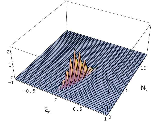
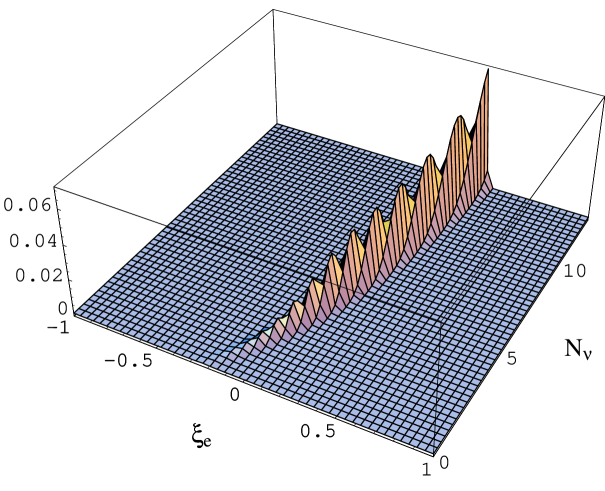
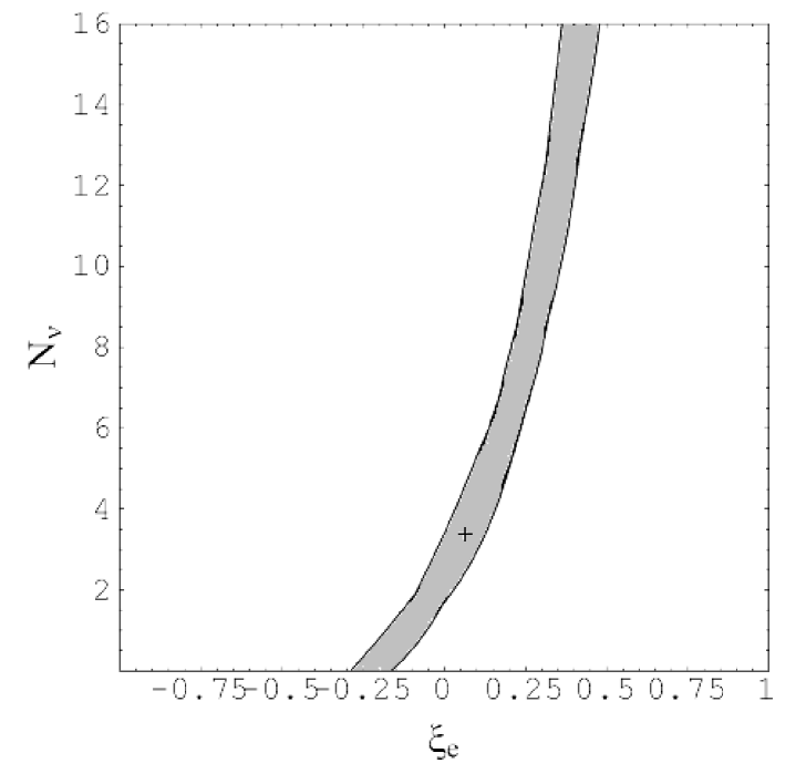
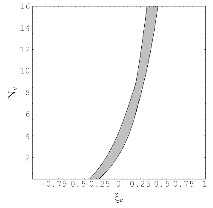
More interesting is to follows the allowed ranges for $\xi_{e}$ and $N_{\nu}$ as functions of $\eta$. In Figures 17 and 18 we show ${\cal L}(\xi_{e},\,N_{\nu},\,\eta_{10})$, evaluated for $\eta_{10}$ taking the values in (4.12) and (4.13). Increasing $\eta_{10}$ in the considered range, the likelihood functions move towards higher values of $\xi_{e}$ and $N_{\nu}$, along, approximatively, a linear path. This is due to the fact that increasing $\xi_{e}$, which results in a lower value for the $n/p$ ratio, and then for $Y_{p}$, must be compensated by a faster expansion produced by a higher value for $N_{\nu}$. This behaviour is highlighted in the $95\%$ exclusion plots for the $\xi_{e}$ and $N_{\nu}$ parameters for different values of $\eta_{10}$, which are reported in Figures 19 and 20 with the bound $N_{\nu}\leq 13$. These two plots summarize our analysis of the degenerate BBN scenario, providing the combined bounds on $\xi_{e}$ and $N_{\nu}$. For low $D$ the allowed range for $\eta_{10}$ is $3.3\div 9.9$, while for high $D$ we have $1.1\div 5.8$. In both cases the degenerate BBN scenario, at $2\sigma$ level is compatible with observational results on nuclide abundances even for quite large values for both $N_{\nu}$ and $\xi_{e}$. As expected, however, these two parameters are strongly correlated.

From our analysis we see that a large value for $\eta\sim 10^{-9}$ is compatible, at $2\sigma$ level, with degenerate BBN for quite large $N_{\nu}$ only, $N_{\nu}\geq 10$, and large positive $\xi_{e}\geq 0.3$. The BOOMERANG and MAXIMA-1 results seem to indicate a value for $\eta\sim 10^{-9}$, but at the same time suggest $N_{\nu}\leq 13$, again at $2\sigma$ level [34]. We may conclude that the degenerate BBN scenario and BOOMERANG and MAXIMA-1 results are compatible only in the very top area in the exclusion plot of Figure (19) for the low $D$ scenario. In the high $D$ case, the upper limit on $N_{\nu}$ is already reached for $\eta\sim 6.5{\cdot}10^{-10}$. As a conclusion we can say that, if the result $\eta\sim 10^{-9}$ will be confirmed, the degenerate BBN scenario is not consistent with CMBR results at $2\sigma$ level, while there is agreement for the low $D$ case. For slightly lower values for $\eta\sim(0.5\div 0.6)10^{-10}$, which corresponds to the central value measured by MAXIMA-1 experiment, the agreement at $2\sigma$ level definitely improves, and it would represent a signal in favour of a large neutrino–antineutrino asymmetry in the universe, $0.2\leq\xi_{e}\leq 0.5$ and $N_{\nu}\geq 10$ [35]. We note that a similar result has been obtained in [36].

5 Conclusions

In this paper we have reported the results of a likelihood analysis of Big Bang Nucleosynthesis theoretical predictions versus the experimental data, both for vanishing neutrino chemical potentials (standard BBN) and in presence of neutrino-antineutrino asymmetries (degenerate BBN). The theoretical estimates have been obtained by using a new updated code we have developed in the recent years to increase the accuracy at the $1\%$ level.

In the standard scenario, BBN predictions are in good agreement with experimental data for both low and high $D$ results. In the first case, since $Y_{D}$ is a decreasing function of baryonic asymmetry $\eta$, the low Deuterium abundance fixes the maximum of total likelihood to larger values of $\eta$, and to compensate the effect on $Y_{p}$ yields smaller values of $N_{\nu}$. In this way we have obtained as preferred values $N_{\nu}=2.44$ and $\eta_{10}=4.69$. The situation is reversed for high $D$ where the maximum lies at $N_{\nu}=3.29$ and $\eta_{10}=1.81$. From the plots of $95\%$ CL for both the above likelihood functions one gets the corresponding compatibility regions

$$\begin{array}[]{ccccc}\mbox{low}~{}D&1.7\leq N_{\nu}\leq 3.3&&4.0\leq\eta_{10}\leq 5.7&\,\,\,0.015\leq\Omega_{B}h^{2}\leq 0.021\\ &&&&\\ \mbox{high}~{}D&2.3\leq N_{\nu}\leq 4.4&&1.4\leq\eta_{10}\leq 3.7&\,\,\,0.005\leq\Omega_{B}h^{2}\leq 0.014\end{array}~{}~{}~{}.$$ (5.17)

Both ranges on $N_{\nu}$ are comparable with the results of Ref. [4]. For the baryon asymmetry $\eta$, the result for low $D$ fairly coincides with [4], whereas the distortion of the contour for $95\%$ CL in case of high $D$ makes our upper limit on $\eta_{10}$ larger than the value of [4]. This effect is mainly due to the non-trivial dependence on the parameters $N_{\nu}-\eta_{10}$ of the nuclear theoretical uncertainties.

We have also analyzed the degenerate BBN scenario, motivated by the BOOMERANG and MAXIMA-1 results [24] on the CMBR spectrum. For both high and low Deuterium measurements we have obtained a $2\sigma$ exclusion plots for the $\xi_{e}$ and $N_{\nu}$ parameters, and we have shown that the theoretical estimates are in good agreement with the experimental measurements of light nuclei abundances even for large values of these parameters, provided they lie in the regions shown in Fig.s (19) and (20). In particular large values for $\eta$ implies high values for the neutrino degeneracy parameters.

A first analysis of the recent CMBR data, [24], suggests quite large values for $\eta\sim 10^{-9}$. From our results we see that this baryon to photon density is actually too high to be in good agreement with degenerate BBN, the compatibility being only at $2\sigma$ level, with the low Deuterium scenario. This conclusion holds if we constraint the effective number of neutrinos to be bounded by $N_{\nu}\leq 13$, which, as pointed out in [34], is again suggested by BOOMERANG data. The agreement improves for slightly smaller values for $\eta$, as the central value obtained by MAXIMA-1 results, and would be an evidence in favour of large neutrino degeneracy, $0.2\leq\xi_{e}\leq 0.5$, $N_{\nu}\geq 10$, an intriguing feature of the neutrino cosmic background. New experimental results, as the one expected from the MAP and PLANCK experiments on CMBR, as well as new analysis of the BOOMERANG and MAXIMA-1 data, will be crucial in clarifying this issue.

Acknowledgements
The authors are pleased to thank Dr.s Sergio Pastor, Marco Peloso and Francesco Villante for useful discussions and comments. We thank A. Bottino for pointing us the MAXIMA-1 Collaboration results, and M. Kaplinghat for valuable remarks.

Appendix A Series expansion for integral quantities

The partial derivatives of $L$ with respect to $z$ and ${\phi_{e}}$, $L_{z}$ and $L_{{\phi_{e}}}$, can be expressed as the following series

$$L_{z}(z,\,{\phi_{e}})=\frac{dz_{R}}{dz}~{}\left\{\frac{2\,L}{z_{R}}-\left(\frac{z_{R}}{\pi}\right)^{2}\sum_{n=1}^{\infty}~{}(-1)^{n+1}~{}\left[K_{1}(n\,z_{R})+K_{3}(n\,z_{R})\right]\,\sinh(n\,{\phi_{e}})\right\},$$ (A.1)

$$L_{{\phi_{e}}}(z,\,{\phi_{e}})=\frac{2\,z_{R}^{2}}{\pi^{2}}~{}\sum_{n=1}^{\infty}~{}(-1)^{n+1}~{}K_{2}(n\,z_{R})\,\cosh(n\,{\phi_{e}})~{}~{}~{},~{}~{}~{}~{}~{}~{}~{}~{}~{}~{}~{}~{}~{}~{}~{}~{}~{}$$ (A.2)

where the $K_{i}$ are the modified Bessel functions of the second kind and in $z_{R}(z)=m_{e}^{R}/T$ we consider the renormalized electron mass,

$$m_{e}^{R}(T)\simeq m_{e}~{}\left[1+\frac{\pi}{3}\,\alpha~{}\left(\frac{T}{m_{e}}\right)^{2}\right].$$ (A.3)

The series expansion for the remaining electron quantities are

$$\hat{\rho}_{e}(z,\,{\phi_{e}}) = \frac{z_{R}^{3}}{2\,\pi^{2}}~{}\sum_{n=1}^{\infty}~{}\frac{(-1)^{n+1}}{n}~{}\left[3\,K_{3}(n\,z_{R})+K_{1}(n\,z_{R})\right]\,\cosh(n\,{\phi_{e}})~{}~{}~{},$$ (A.4)

$$\frac{\delta\hat{\rho}_{e}}{\delta z}(z,\,{\phi_{e}}) = \frac{dz_{R}}{dz}~{}\biggl{\{}\frac{3\,\hat{\rho}_{e}}{z_{R}}+\frac{z_{R}^{3}}{2\,\pi^{2}}\sum_{n=1}^{\infty}~{}(-1)^{n+1}~{}\biggl{[}\frac{15\,K_{3}(n\,z_{R})+K_{1}(n\,z_{R})}{n\,z_{R}}$$ (A.5)

$$-4\,K_{4}(n\,z_{R})\biggr{]}\,\cosh(n\,{\phi_{e}})\biggr{\}}~{}~{}~{},$$

$$\frac{\delta\hat{\rho}_{e}}{\delta{\phi_{e}}}(z,\,{\phi_{e}}) = \frac{z_{R}^{3}}{2\,\pi^{2}}~{}\sum_{n=1}^{\infty}~{}(-1)^{n+1}~{}\left[3\,K_{3}(n\,z_{R})+K_{1}(n\,z_{R})\right]\,\sinh(n\,{\phi_{e}})~{}~{}~{}.$$ (A.6)

Figure 1: The Deuterium abundance $Y_{D}$ (3.2), for $N_{\nu}=3$, versus $\eta_{10}\equiv 10^{10}\eta$. The horizontal bands correspond to the experimental determinations of Ref.s [5, 6]. The solid lines bound the theoretical predictions at $1\sigma_{th}$. The dashed line, on this scale indistinguishable from the central solid line, is the result from [22]. No result is given for $D$ in [12]. The same notation has been applied in the following Figures.

Figure 2: Relative difference (in percent) for Deuterium abundance between the results of the present work and the ones from [22] in the case $N_{\nu}=3$.

Figure 3: The helium-3 abundance $Y_{{}^{3}He}$ (3.2), for $N_{\nu}=3$, versus $\eta_{10}$. The dashed line is the result from [22]. No result is given for ${}^{3}He$ in [12].

Figure 4: Relative difference (in percent) for $Y_{{}^{3}He}$ between the results of present work and the ones from [22] in the case $N_{\nu}=3$.

Figure 5: The helium-4 mass fraction $Y_{p}$ (3.3), for $N_{\nu}=3$, versus $\eta_{10}$. The dashed line is the result from [12] and the dotted one from [22].

Figure 6: Relative difference (in percent) for $Y_{p}$ between the results of present work and the ones from [22] (solid line) and from [12] (dashed line) in the case $N_{\nu}=3$.

Figure 7: The lithium-7 abundance $Y_{{}^{7}Li}$ (3.2), for $N_{\nu}=3$, versus $\eta_{10}$. The dashed line, on this scale indistinguishable from the central solid line, is the result from [22]. No result is given for ${}^{7}Li$ in [12].

Figure 8: Relative difference (in percent) for $Y_{{}^{7}Li}$ between the results of present work and the ones from [22] in the case $N_{\nu}=3$.

Figure 9: Total likelihood function (3.6) versus $N_{\nu}-\eta_{10}$ for the low experimental value of $D$ [5].

Figure 10: Contour plots of the total likelihood function for the low experimental value of $D$. From inner to outer they correspond to $50\%$, $68\%$ and $95\%$ CL, respectively. The cross indicates the maximum of likelihood function, and corresponds to $N_{\nu}=2.44$ and $\eta_{10}=4.69$.

Figure 11: Total likelihood function versus $N_{\nu}-\eta_{10}$ for the high experimental value of $D$ [6].

Figure 12: Contour plots of the total likelihood function for the high experimental value of $D$. From inner to outer they correspond to $50\%$, $68\%$ and $95\%$ CL, respectively. The cross corresponds to $N_{\nu}=3.29$ and $\eta_{10}=1.81$.

Figure 13: Single likelihood functions for the three light abundances in the case of the low experimental value of $D$ and $N_{\nu}=3.29$. The single peaked curve stands for $L_{D}$, the double peaked curve for $L_{{}^{7}Li}$ and the broad one for $L_{{}^{4}He}$. The same notation holds for the following figures.

Figure 14: Single likelihood functions for the three light abundances in the case of the low experimental value of $D$ and $N_{\nu}=2.44$.

Figure 15: Single likelihood functions for the three light abundances in the case of the high experimental value of $D$ and $N_{\nu}=3.29$.

Figure 16: Single likelihood functions for the three light abundances in the case of the high experimental value of $D$ and $N_{\nu}=2.44$.

Figure 17: Total likelihood function in the degenerate BBN scenario in the plane $\xi_{e}$-$N_{\nu}$, in the case of the low experimental value of $D$ for $\eta_{10}=5$.

Figure 18: Total likelihood function in the degenerate BBN scenario, in the case of the high experimental value of $D$ for $\eta_{10}=4.20$.

Figure 19: The $95\%$ exclusion plot for the variables $\xi_{e}-N_{\nu}$ for low $D$ experimental value. The dark area represents the BBN allowed region, for $\eta_{10}$ in the range $3.3\div 9.9$. The cross corresponds to the maximum of the likelihood function.

Figure 20: The $95\%$ exclusion plot for the variables $\xi_{e}-N_{\nu}$ for high $D$ experimental value. The dark area represents the BBN allowed region, for $\eta_{10}$ in the range $1.1\div 5.8$. The cross corresponds to the maximum of the likelihood function.

References

- [1] R.V. Wagoner, W.A. Fowler, and F. Hoyle, Astrophys. J. 148 (1967) 3; R.V. Wagoner, Astrophys. J. Suppl. 18 (1969) 247; R.V. Wagoner, Astrophys. J. 179 (1973) 343.
- [2] B.E.J. Pagel, E.A. Simonson, R.J. Terlevich and M. Edmunds, Mon. Not. Roy. Astron. Soc. 255 (1992) 325; E. Skillman and R.C. Kennicutt, Astrophys. J. 411 (1993) 655; E. Skillman, R.J. Terlevich, R.C. Kennicutt, D.R. Garnett, and E. Terlevich, Astrophys. J. 431 (1994) 172; K.A. Olive and G. Steigman, Astrophys. J. Suppl. 97 (1995) 49.
- [3] Y.I. Izotov and T.X. Thuan, Astrophys. J. 500 (1998) 188.
- [4] K.A. Olive, G. Steigman and T.P. Walker, submitted to Phys. Rept., astro-ph/9905320.
- [5] R.F. Carswell, M. Rauch, R.J. Weymann, A.J. Cooke, and J.K. Webb, MNRAS 268 (1994) L1; A. Songaila, L.L. Cowie, C. Hogan, and M. Rugers, Nature 368 (1994) 599; M. Rugers and C.J. Hogan, A.J. 111 (1996) 2135; R.F. Carswell, et al. MNRAS 278 (1996) 518; E.J. Wampler, et al., A.A. 316 (1996) 33; J.K. Webb, R.F. Carswell, K.M. Lanzetta, R. Ferlet, M. Lemoine, A. Vidal-Madjar, and D.V. Bowen, Nature 388 (1997) 250.
- [6] S. Burles and D. Tytler, Astrophys. J. 499 (1998) 689.
- [7] J.A. Thorburn, Astrophys. J. 421 (1994) 318.
- [8] P. Molaro, F. Primas and P. Bonifacio, Astron. Astrophys. 295 (1995) L47.
- [9] P. Bonifacio and P. Molaro, Mon. Not. Roy. Astron. Soc. 285 (1997) 847.
- [10] L. Kawano, preprint FERMILAB-Pub-88/34-A; preprint FERMILAB-Pub-92/04-A.
-
[11]
For a list of the relevant nuclear rates see the Web
sites
http://www.phy.ornl.gov/astrophysics/data/data.html, http://pntpm.ulb.ac.be/Nacre/barre_database.htm. - [12] R.E. Lopez and M.S. Turner, Phys. Rev. D59 (1999) 103502.
- [13] S. Esposito, G. Mangano, G. Miele and O. Pisanti, Nucl. Phys. B568 (2000) 421.
- [14] S. Esposito, G. Mangano, G. Miele and O. Pisanti, Nucl. Phys. B540 (1999) 3.
- [15] A. Sirlin, Phys. Rev. 164 (1967) 1767.
- [16] W.J. Marciano and A. Sirlin, Phys. Rev. Lett. 46 (1981) 163; Phys. Rev. Lett. 56 (1986) 22.
- [17] D. Seckel, preprint BA-93-16, hep-ph/9305311; R. E. Lopez, M. S. Turner and G. Gyuk, Phys. Rev. D56 (1997) 3191.
- [18] D.A. Dicus, E.W. Kolb , A.M. Gleeson, E.C.G. Sudarshan, V.L. Teplitz and M.S. Turner, Phys. Rev. D26 (1982) 2694; J.L. Cambier, J.R. Primack and M. Sher, Nucl. Phys. B209 (1982) 372; J.F. Donoghue, B.R. Holstein and R.W. Robinett, Ann. Phys. (N.Y.) 164 (1985) 23; J.F. Donoghue and B.R. Holstein, Phys. Rev. D28 (1983) 340 and Phys. Rev. D29 (1984) 3004; A.E. Johansson, G. Peresutti and B.S. Skagerstam, Nucl. Phys. B278 (1986) 324; W. Keil, Phys. Rev. D40 (1989) 1176; R. Baier, E. Pilon, B. Pire and D. Schiff, Nucl. Phys. B 336 (1990) 157; W. Keil and R. Kobes, Physica A 158 (1989) 47; M. LeBellac and D. Poizat, Z. Phys. C47 (1990) 125; T. Altherr and P.Aurenche, Phys. Rev. D40 (1989) 4171; R.L. Kobes and G.W. Semeneff, Nucl. Phys. B260 (1985) 714 and B272 (1986) 329; R.F. Sawyer, Phys. Rev. D53 (1996) 4232; I.A. Chapman, Phys. Rev. D55 (1997) 6287; S. Esposito, G. Mangano, G. Miele and O. Pisanti, Phys. Rev. D58 (1998) 105023.
- [19] J.J. Kapusta, Finite-Temperature Quantum Field Theory, Cambridge University Press, Cambridge, 1989.
- [20] M.A. Herrera and S. Hacyan, Astrophys. J. , 336 (1989) 539, N.C. Rana and B. Mitra, Phys. Rev. D44 (1991) 393; N.Y. Gnedin and O.Y. Gnedin, Astrophys. J. 509 (1998) 11; S. Hannestad and J. Madsen, Phys. Rev. D52 (1995) 1764; A.D. Dolgov, S.H. Hansen and D.V. Semikoz, Nucl. Phys. B 503 (1997) 426; B. Fields, S. Dodelson and M.S. Turner, Phys. Rev. D47 (1993) 4309.
- [21] L.M. Krauss and P. Romanelli, Astrophys. J. 358 (1990) 47; P.J. Kernan and L.M. Krauss, Phys. Rev. Lett. 72 (1994) 3309.
- [22] G. Fiorentini, E. Lisi, S. Sarkar and F.L. Villante, Phys. Rev. D58 (1998) 063506; E. Lisi, S. Sarkar and F.L. Villante, Phys. Rev. D59 (1999) 123520.
- [23] H. Kang and G. Steigman, Nucl. Phys. B372 (1992) 494.
- [24] P. De Bernardis et al. (BOOMERANG Collaboration) Nature 404 (2000), 955; A.E. Lange et al. (BOOMERANG collaboration), astro-ph/0005004; S. Hanany et al. (MAXIMA Collaboration), astro-ph/0005123; A. Balbi et al. (MAXIMA Collaboration), astro-ph/0005124.
- [25] K. Enqvist, K. Kainulainen and V. Semikoz, Nucl. Phys. B374 (1992) 392.
- [26] The code can be found at the Web site http://www-thphys.physics.ox.ac.uk/users/ SubirSarkar/bbn.html.
- [27] I. Affleck and N. Dine, Nucl. Phys. B249 (1985) 361.
- [28] A. Casas, W.Y. Cheng and G. Gelmini, Nucl. Phys. B538 (1999) 297.
- [29] J. March-Russell, H. Murayama and A. Riotto, JHEP 11 (1999) 015.
- [30] J. MacDonald, Phys. Rev. Lett. 84 (2000) 4798.
- [31] R. Foot and R.R. Volkas, Phys. Rev. D56 (1997), 6653; R. Foot, Phys. Rev. D61 (2000) 023510; P. Di Bari and R. Foot, Phys. Rev. D61 (2000) 105012.
- [32] D.P. Kirilova and M.V. Chizhov, Phys. Lett. B393 (1997), 375; A.D. Dolgov, S.M. Hansen, S. Pastor and D.V. Semikoz, hep-ph/9910444.
- [33] S. Esposito, G. Miele, S. Pastor, M. Peloso and O. Pisanti, preprint DSF-16/2000 , SISSA-51/2000/EP, astro-ph/0005573.
- [34] S. Hannestad, astro-ph/0005018.
- [35] J. Lesgourgues and M. Peloso, astro-ph/0004412.
- [36] M. Orito, T. Kajino, G.J. Mathews and R.N. Boyd, astro-ph/0005446.