Temporal properties of flares in accretion disk coronae

Abstract

Using a non-linear Monte-Carlo code we investigate the radiative response of an accretion disk corona system to static homogeneous flares. We model a flare by a rapid (comparable to the light crossing time) energy dissipation in the corona or the disk.

If the flares originate from the disk, the coronal response to the soft photon shots produces a strongly non-linear Comptonised radiation output, with complex correlation/anti-correlations between energy bands. This behavior strongly differs from those found with usual linear calculations. Thus any model for the rapid aperiodic variability of X-ray binaries invoking a varying soft photon input as a source for the hard X-ray variability has to take into account the coronal temperature response.

On the other hand, if the flare is due to a violent heating of the corona, when the perturbation time scale is of the order of a few corona light crossing times, the shot spectrum evolves from hard to soft. This general trend is independent of the shot profile and geometry. We show that for short dissipation time, the time averaged spectra are generally harder than in steady state situation. In addition, annihilation line and high energy tails can be produced without need for non-thermal processes.

1 Introduction

The hard X/$\gamma$-ray spectra of galactic black hole candidates (GBHC) in their low hard state as well as Seyfert galaxies can be generally represented as a sum of a hard power-law continuum with a cutoff at a few hundred keV and a Compton reflection bump (with a Fe K$\alpha$ line at $\sim 6.4$ keV) produced when high energy photons interact with cold material (Zdziarski et al. 1996). The presence of the Compton reflection component (Guilbert & Rees 1988; George & Fabian 1991) implies that cold material could be present in the direct vicinity of the X/$\gamma$-ray producing region. A soft excess present below $\sim 1$ keV is usually associated with the thermal emission from the cold accretion disk and can be powered by the viscous dissipation in the disk itself as well as by reprocessing hard photons. These three components are generally interpreted in the framework of accretion disk corona models. These models assume that the soft thermal radiation is emitted by the disk and then Comptonised in a very hot plasma, the “corona”. The reflection features arise naturally from the disk illumination. The nature and geometry of the corona are unclear. Several geometries have been proposed: slab sandwich-like corona (Haardt & Maraschi, 1991, 1993), localized active regions on the disk surface powered by magnetic reconnections (Liang et al. 1977; Galeev et al. 1979; Haardt et al. 1994) or a hot accretion disk in the center surrounded by a cold standard disk (Shapiro et al. 1976 ; Ichimaru 1977; Narayan & Yi 1994). Unfortunately, spectroscopy alone does not allow one to firmly probe either the geometry or the way the corona is powered.

X-ray variability studies seem to be a key for the understanding of accretion processes around compact objects. They should at least bring indications on the nature and structure of the corona. The short term variability of black hole X-ray binaries is now well known thanks to an impressive amount of observational data accumulated since many years by several space experiments (Cui 1999). There is however no accepted model that accounts for most of the observational data. The inner disk dynamic predicts important variability at kHz frequencies while a stronger variability is observed around 1 Hz. The power density spectrum is roughly a power-law of index between -1.0 and -2.0. Another important feature of the temporal behavior is the time lags between hard and soft photons that depend on Fourier frequency $\propto f^{-1}$. Whether the intrinsic source of the variability is the disk (Payne 1980; Miyamoto et al. 1988) or the corona (Haardt et al. 1997, Poutanen & Fabian 1999) is still a matter of debate. As the characteristic time scales are expected to grow linearly with the black hole mass, the time scales are far longer in Seyfert galaxies. The long observations required prevent the acquisition of as many data as for X-ray binaries. Their Power Density Spectra (PDS), at least, are similar to those of stellar black holes, modulo the mass scale factor (Edelson & Nandra 1999).

To understand these temporal characteristics it seems important to introduce the temporal dimension in spectral models. The most important difficulty when dealing with time dependent problems is that the system is not necessarily in radiative equilibrium. The corona is strongly coupled with radiation, its physical parameters such as temperature and optical depth can fluctuate in response to changes in the photon field. These variations in turn influence the radiative field, making the system strongly non-linear. The dynamics of compact plasma has been extensively studied during the eighties in the context of the models for the high energy emission of active galactic nuclei; first using analytical arguments (Guilbert et al. 1983), then using more and more accurate numerical methods (Guilbert & Stepney 1985; Fabian et al. 1986; Kusunose 1987; Done & Fabian 1989). The most detailed treatment of micro-physics was achieved by Coppi (1992) using a method based on the solution of the kinetic equations. These studies gave an understanding of the behaviour of the plasma and the spectral evolution of the emitted radiation, when the input parameters (heating, external soft-photons injection…) vary on time scales of the order of the light crossing time.

However, at the time of those studies the importance of the coupling with cold matter did not appear as crucial as it does now. Indeed, in the accretion disk corona framework, another complication appears: the hard X-ray radiation is produced by Comptonisation of soft photons that, in turn, can be mostly produced by reprocessing the same hard radiation in the cold accretion disk (the “feedback” mechanism). Until now, in most studies only steady-state situations have been considered. The physical characteristics of the emitting region (such as temperature and optical depth of the Comptonising cloud) that determine the observed X/$\gamma$-ray spectrum are assumed not to vary in time (e.g. Sunayev & Titarchuk 1980). The most detailed calculations considered only steady states, where the temperature and the optical depth are defined by the energy balance and electron-positron pair balance, assuming a constant heating (Haardt & Maraschi 1993; Stern et al. 1995a,b; Poutanen & Svensson 1996).

The observed rapid spectral changes imply the presence of rapid changes in the physical conditions of the source. When taken into account in radiative transfer modeling, these changes have been considered as a succession of steady state equilibria (Haardt et al. 1997; Poutanen & Fabian 1999). This approximation is acceptable as long as the underlying perturbation evolves on time scales, $t_{\mathrm{c}}$, far larger than the light crossing time. Actually, we do not know if this assumption is valid.

Here we aim at giving a first look at the rapid spectral and temporal evolution of a hot plasma coupled with a reprocessor. In this first attempt to model the non-linear behavior of a time dependent accretion disk corona system, we try to point out the main properties of the accretion disk corona when the dissipation parameters change on time scales of the order of the light crossing time of the corona. We show that the non-linear Monte Carlo method (Stern et al. 1995a) can be an efficient tool to perform the task of computing the time evolution of the plasma parameters together with a detailed radiative transfer treatment enabling the production of light curves. Our model assumptions are presented in Sect. 2.

Section  3 gives a description of our computational method. The different consistency tests that we performed in order to check the validity of the code for steady state situations are presented in Sect. 4. Then we present some applications to time dependent situations. We first investigate the case of an equilibrium modified by a variation in the soft photon input, in Sect.  5. In Sect. 6, we then consider situations where the energy dissipation in the corona occurs during short flares.

2 Model assumptions

2.1 The slab corona model

We consider a simple slab geometry for the corona. The corona is composed of electrons (associated with ions) with a fixed Thomson optical depth $\tau_{\mathrm{s}}$. This corona is assumed to be uniformly heated by an unspecified process, which is quantified using the usual local dissipation parameter $l_{\mathrm{c}}=HF_{\mathrm{h}}\sigma_{\mathrm{T}}/m_{\mathrm{e}}c^{3}$, where $F_{\mathrm{h}}$ is the power supplied in the corona per unit area, $H$ the height of the slab, $\sigma_{\mathrm{T}}$ the Thomson cross section, $m_{\mathrm{e}}$ the electron rest mass and $c$ the speed of light.

The corona cools by Comptonisation of the soft radiation from the disk. The balance between heating and cooling leads to a mean temperature $T_{\mathrm{e}}$. Due to photon-photon interactions, $e^{+}/e^{-}$ pairs can appear in the corona leading to a total optical depth $\tau_{\mathrm{T}}>\tau_{\mathrm{s}}$ that is governed by the balance between pair production and annihilation.

The disk emission arises from two processes:

• internal viscous dissipation parametrized by the disk compactness $l_{\mathrm{d}}=HF_{\mathrm{s}}\sigma_{\mathrm{T}}/m_{\mathrm{e}}c^{3}$, where $F_{\mathrm{s}}$ is the intrinsic flux of radiation emitted by the disk with a blackbody spectrum at fixed temperature $T_{\mathrm{bb}}$.

• reprocessing of Comptonised radiation coming from the corona. Most of the impinging radiation is absorbed and thermally re-emitted with blackbody temperature $T_{\mathrm{bb}}$, a fraction is Compton reflected forming a hump in the high energy spectrum.

2.2 Steady state properties

The equilibrium properties of accretion disk corona have been extensively studied (Haardt & Maraschi 1993; Stern et al. 1995a, b; Poutanen & Svensson 1996; Dove et al. 1997b). Let us recall their main characteristics.

For a given total optical depth $\tau_{\mathrm{T}}$, the plasma temperature and thus the spectral properties depend only on the ratio $l_{\mathrm{d}}/l_{\mathrm{c}}$ and are independent of the absolute luminosity. When $l_{\mathrm{d}}/l_{\mathrm{c}}\gg 1$, heating is negligible, the plasma is at Compton temperature driven by the disk thermal radiation $T_{\mathrm{e}}\sim T_{\mathrm{r}}$. Decreasing $l_{\mathrm{d}}/l_{\mathrm{c}}$ quickly raises the temperature provided that $l_{\mathrm{d}}/l_{\mathrm{c}}>0.1$. For smaller values of the ratio $l_{\mathrm{d}}/l_{\mathrm{c}}$, the temperature becomes independent of $l_{\mathrm{d}}/l_{\mathrm{c}}$. It is easily understandable since the cooling is then dominated by the reprocessed photons whose energy density grows linearly with the heating rate $l_{\mathrm{c}}$. For a given optical depth there is thus a maximum self-consistent temperature. This maximum temperature depends only on the feedback coefficient which is defined as the fraction of the X-ray flux which reenters the source as soft radiation after reprocessing. This feedback coefficient depends mainly on the geometry. Thus for a given geometry the hardness of the emitted spectra is limited by the maximum temperature achievable.

Based on these arguments, it has been often argued that the slab geometry produces too steep spectral slopes to account for the observed spectra in black hole binaries and Seyfert galaxies (Stern et al. 1995b; Dove et al. 1997b; Poutanen et al. 1997). The geometry is more likely a spherical corona surrounded by the cold accretion disk, or constituted of small active regions at the surface of the disk. In these cases indeed the feedback coefficient is lower. Note, however, that slab corona could be consistent with observations if the disk is ionised (Nayakshin & Dove 1999; Ross et al. 1999) or if there is a bulk motion of plasma away from the disk (Beloborodov 1999).

Decreasing $\tau_{\mathrm{s}}$ raises the temperature since the injected energy is shared by a smaller number of particles. If $l_{\mathrm{c}}/\tau_{\mathrm{s}}>1$ and $l_{\mathrm{d}}/l_{\mathrm{c}}\ll 1$, the pair production can increase significantly the total optical depth $\tau_{\mathrm{T}}$. Then the equilibrium optical depth has to be computed using the pair production and annihilation balance and will depend on the compactness $l_{\mathrm{c}}$. An increase in $l_{\mathrm{c}}$ increases the pair production rate and so $\tau_{\mathrm{T}}$ which in turn decreases the temperature.

2.3 Time dependent situations

Here we will consider rapid changes in $l_{\mathrm{c}}$ or $l_{\mathrm{d}}$. The dissipation parameters $l_{\mathrm{c}}$ and $l_{\mathrm{d}}$ are thus functions of time with a characteristic time scale of a few $H/c$.

Even if the simple slab geometry considered here seems rather unrealistic with regard to the observations, we do not expect that the general features presented here change qualitatively for a different geometry.

To simplify our calculations, we made several approximations discussed below:

First, we assume thermal electron distributions. It is well known that if the temperature changes are too fast the particles may not have time to form a true Maxwellian distribution. The main consequence is the formation of a high-energy tail in the electron distribution (Li et al. 1996; Poutanen & Coppi 1998) that could explain the emission observed at gamma-ray energies in black hole candidate Cygnus X-1 (Ling et al. 1997; McConnell et al. 1997). Unless the medium is very optically thin, the hard-X ray spectrum should not be significantly affected. Indeed, the Comptonisation spectrum is mainly sensible to the mean electron energy and not to the detailed particle distribution when multiple scattering is important (Ghisellini et al. 1993).

We also neglect the time delays due to the radiative transfer in the disk. The reprocessing and reflection are supposed to be instantaneous. The travel time for a photon in the disk scales as the inverse of the disk density. The disk being dense and optically thick, the time delays due to light traveling time in the disk are negligible compared to the corona light crossing time. Concerning the reprocessed component the delays are mainly due to the thermalisation time of the disk which is short (typically $\sim 10\mu$s, see e.g. Nowak et al. 1999) compared to the corona light crossing time.

Another important simplification is that the blackbody temperature of the disk is fixed and considered to be constant. We can expect that the disk temperature will have important fluctuations (scaling as $l^{1/4}$) as a response to changes in the illuminating flux or the intrinsic dissipation parameter. Note however that we take into account the disk luminosity variations in a self-consistent manner. Our specification of a fixed temperature fixes only the disk spectrum shape and not its amplitude.

We thus expect that calculations including the temperature changes would give different results only for the spectral evolution in the soft X-ray bands ($<$ 1 keV). At higher energy where the flux is dominated by Compton emission, the results should not be affected. Indeed, at first order, the Compton losses scale as the soft photon energy density rather than photon energy. We checked that the temporal evolution is not qualitatively sensible to the value of the fixed blackbody temperature, which can fluctuate within a factor of 10 without changing significantly the high-energy light curves. For detailed quantitative considerations, however, these effects will have to be implemented in the code.

3 Monte-Carlo Code

To compute the evolution of $T_{\mathrm{e}}$ and $\tau_{\mathrm{T}}$ together with the flare light curves, we use a Non-Linear Monte-Carlo code (NLMC) that we developed according to the Large Particle (LP) method proposed by Stern et al. (1995a) . The main features of our code are similar to Stern’s. The radiative processes taken in account are Compton scattering, pair production and annihilation. A pool is used to represent the thermal electron population. The reflection component is computed with a coupled linear code (Jourdain & Roques 1995; Malzac et al. 1998). We implemented in our NLMC code the slab corona described in Stern et al (1995b) (see also Dove et al. 1997a). The slab is divided into ten homogeneous layers to account for its vertical structure.

An ample discussion of the LP method can be found in Stern et al. (1995a,b) and further details on its application to thermal accretion disk corona models can be found in Dove et al. (1997a), we only discuss here the aspects of our code which are related to temporal variability.

Unlike standard Monte-Carlo Methods (Pozdnyakov et al. 1983; Gorecki & Wilczewski 1984), the LP method propagates all the particles in a parallel and synchronized way. Thus, the time variable appears as a natural parameter. However, when dealing with time-dependent (TD) systems the problem of statistical errors becomes crucial. Indeed, when simulating a stationary system the spectrum has just to be integrated over a longer time (in LP method) or over more particles (in a standard MC method) to get the required statistical accuracy. In TD situations this is of course not the case and the statistical accuracy depends on the number of LP, $N_{\mathrm{LP}}$, used to represent the system at a given time. Due to the weighting technique used, we do not require a very large number of LPs to get a statistically acceptable representation of the particles distribution inside the active region (here we use 5 10⁴ to 15 10⁴ LPs). However, the number of escaping photon LPs per time step is only a very small fraction of $N_{\mathrm{LP}}$ ($\sim\Delta tN_{\mathrm{LP}}$, $\Delta t=10^{-3}H/c$ here). This prevents the averaging of light curves over too short time scales or too narrow energy ranges.

It is difficult to improve accuracy by increasing the number of LPs, $N_{\mathrm{LP}}$. Indeed the statistical errors scale roughly as $1/\sqrt{N_{\mathrm{LP}}}$. Thus, in order to decrease these errors by a factor of 2, $N_{\mathrm{LP}}$ has to be increased by a factor of 4. The simulation time can be estimated scaling as $N_{\mathrm{LP}}\log{N_{\mathrm{LP}}}$ (Stern et al. 1995a), the performances are thus degraded by more than a factor of 4. This is not negligible particularly when the CPU time is already large (as large as 1 day).

However in our case, we are mainly interested in the average spectrum during a flare, and the light curves averaged over $0.1H/c$ and a decade in energy are sufficient to get the general properties of the flare.

Another problem due to the statistical method is the determination of the electron pool parameters $T_{\mathrm{e}}$ and $\tau_{\mathrm{T}}$. We have to calculate the pool energy $\Delta E_{\mathrm{p}}$ and optical depth changes $\Delta\tau_{\mathrm{T}}$ during $\Delta t$. If this is done using the Monte-Carlo interactions that occurred during the time step, we get huge statistical fluctuations. To limit these fluctuations, Stern et al. (1995a) average the temperature over previous time steps. This method, rigorous only for equilibrium states, introduces in TD simulations an artificial relaxation time. We overcome the problem by computing $\Delta E_{\mathrm{p}}$ and $\Delta\tau_{\mathrm{T}}$ analytically. We use the exact thermal annihilation rate given by Svensson (1982) and the formula given by Barbosa (1982) and Coppi & Blandford (1990) to compute and tabulate the exact energy exchange rate between a photon of given energy and a Maxwellian distribution of electrons through the Compton process. These results are used at the beginning of each time step to evaluate the Compton losses using the updated distribution of photon LPs. This method allows us to limit the step to step fluctuations to less than 1 per thousand. However, statistical fluctuations of the photon distribution can lead to fluctuations of 5 $\%$ on a time scale of a few $H/c$. Fortunately, these oscillations occur only in stationary situations where the electron temperature is more sensitive to photon LP fluctuations. In non-equilibrium situations the temperature is strongly driven toward equilibrium and evolves smoothly.

Figure 1: Comptonisation spectra emitted by a slab corona in energy balance. Disk blackbody temperature $kT_{\mathrm{bb}}$ is 5 eV. Spectra are averaged over inclinations $\theta$ such that $0.6<\cos\theta<0.9$, where $\theta$ is the angle between the line of sight and the disk normal. Solid lines show spectra computed with our code while Stern’s results are shown in dashed lines. Fixed optical depths are, from bottom to top $\tau_{\mathrm{T}}=$0.033, 0.058, 0.090, 0.163 and 0.292. The equilibrium temperatures we found are respectively $kT_{\mathrm{e}}=$425, 300, 225, 152 and 98 keV. Stern’s values for equilibrium temperature are very close to the latter, with the most important difference at $\tau_{\mathrm{T}}=0.163$, for which his temperature is 3$\%$ lower.

4 Validation of the code

4.1 Emitted spectra and energy balance

To check that our code produces accurate Comptonisation spectra, we switched off pair production and annihilation processes and compared our results to spectra from a linear code (see, e.g., Pozdnyakov et al., 1983). In these tests, the energy balance was not considered, optical depth and temperature were fixed. The emergent-angle-dependent spectra as well as the energy and angular distributions of radiation inside the active region, are similar within statistical errors (a few percent). These tests have been performed using a pool to represent the electron distribution. We performed other successful tests when electron LPs are drawn at the beginning of the time step over a fixed distribution (Maxwellian or power law) and for several geometries (sphere, cylinder, slab). Similar comparisons have been performed in the case of a corona coupled with a reprocessor (including the reflection component). Here again a very good agreement was found.

For a slab corona coupled with a disk, taking into account the energy balance provides, for a given optical depth, an equilibrium temperature which can be compared with results from the literature. Stern et al. (1995b) and Poutanen & Svensson (1996) give maximum temperatures which are in agreement with ours within 5 %. Emitted spectra are also in agreement as shown in Fig 1 which compares spectra from our code against results from Stern’s, for the same fixed optical depth, and a temperature determined according to the energy balance.

In addition we tested the energy conservation, by checking that the whole luminosity emitted by the corona+disk system equals the injected power.

These tests validate the treatment of Compton scattering as well as the general architecture of the code and all the routines that do not depend on the type of interaction (LPs management, geometry…), i.e. the main parts of the code.

4.2 Pair production and annihilation

The pair annihilation rate as well as the spectra of produced photons have been compared, in the thermal case, to the analytical formulae given by Svensson (1982) and Svensson et al. (1996). The differences obtained are less than 1 %.

The pair production rate is more difficult to test because it is strongly sensitive to the number density, energy and angular distribution of the photons around and above the electron rest mass energy, $m_{\mathrm{e}}c^{2}$. The pair production rate thus depends strongly on the details of radiative transfer such as the number and shape of spatial cells used (the radiation field being averaged over a cell).

The pair production rate obtained with our NLMC code has been compared with a pair production rate computed analytically from the photon LP distribution provided by the same simulation. Both pair production rates are in agreement within statistical fluctuations (a few percents).

However, detailed comparisons with the results of Stern et al. (1995b) in the framework of accretion disk corona models show important differences for the pure pair plasma case when the optical depth (and compactness) is low ($\tau_{\mathrm{T}}<0.1$). This disagreement leads to differences in optical depth (and thus temperature) up to 25% for $\tau_{\mathrm{T}}\sim 10^{-2}$ ($l_{\mathrm{c}}<1$). The origin of these differences is still not clear; it could be due to differences in the details of the photon-photon interaction treatment, or to the use of a different number of zones, or simply to statistical errors. Indeed Stern et al. (1995a) used 5 times less LPs than we did. However, for less extreme parameters ($l_{\mathrm{c}}>1$), the equilibrium parameters differ by more than 5 % only occasionally. We also tested our equilibrium values against the results presented in the inset of Fig. 2 of Dove et al. (1997a), ($\tau_{\mathrm{s}}=0.2$, $l_{\mathrm{d}}=1$ and $1<l_{\mathrm{c}}<100$), a perfect agreement was found. In addition we performed comparisons with the ISM code (Poutanen & Svensson 1996) for the case of pure pair plasmas in pair and energy balance in slab geometry and found resulting equilibrium optical depths and temperatures differing by less than 10%.

5 Variability driven by the disk

5.1 Set up

The first class of models for the rapid aperiodic variability of GBHC uses the variability of the soft seed photons as a source for the hard X-ray variability (e.g., Kazanas et al. 1997; Hua et al. 1997; Böttcher & Liang 1998). Soft photons are assumed to be injected isotropically in the centre of a very extended corona with a white noise power spectrum. The Compton process wipes out the high frequency variability giving the overall shape of the PSD, and the hard lags are due to the soft photons Compton up-scattering time. Another attractive model of this kind has been recently proposed by B ttcher & Liang (1999) based upon an idea previously quoted by Miyamoto & Kitamoto (1989). In this scheme it is assumed that the soft seed photons are emitted by cool dense blobs of matter spiraling inward through an inhomogenous spherical corona formed by the inner hot disk. These models have however an intrinsic deficiency: they do not account for the energy balance. The comptonising plasma temperature is assumed to be constant while the soft photon field changes very quickly in time. As the Compton scattering on soft photons is the dominant cooling mechanism for the thermal electrons, the temperature is determined mainly by the soft photon energy density $U_{\mathrm{s}}$ and the heating rate. Any modification of the soft photons field induces change in temperature. The cooling time for the thermal electrons is very short, scaling roughly as $1/U_{\mathrm{s}}$. Thus the temperature adjusts very quickly to any significant change in the soft radiation field. These temperature fluctuations in turn affect the emitted spectrum. It is then important to know what really happens when the temperature equilibrium is perturbed by a varying soft photon input.

In our slab corona we consider soft photon flares arising from the disk. We model a flare by a sudden increase in the disk internal dissipation parameter $l_{\mathrm{d}}$.

5.2 Results of simulations

Fig. 2 presents the evolution of the coronal physical parameters in the case of an equilibrium perturbed by a strong and violent emission of soft photons from the disk.

The system is initially in a steady state where the internal disk dissipation parameter $l_{\mathrm{d}}=1$ while $l_{\mathrm{c}}=100$. $l_{\mathrm{d}}$ is then increased by a factor of 100 during $\Delta t=1$ $H/c$ (hereafter time is expressed in $H/c$ units). The Compton cooling of the plasma is quasi-instantaneous and the temperature drops by $\sim 15\%$. The pair production rate thus decreases, leading to a lower optical depth. After perturbation, the optical depth increases again, but slower than the lepton kinetic energy. Thus the temperature increases slowly and reaches a maximum higher than the initial equilibrium temperature. This arises from the pair production time being longer than the heating time. After the event the system relaxes toward equilibrium.

The code also enables us to compute the associated light curves (Fig. 2). The soft luminosity in the lower energy band ($E<$2 keV) increases strongly by a factor of $\sim 2$ around 1 $H/c$ after the beginning of the flare. Note however that this is a small variation compared to the change of a factor 100 in $l_{\mathrm{d}}$ that we imposed. Indeed in the steady state the disk emission is the sum of intrinsic dissipation and reprocessing of hard radiation.

The delay is due to the corona light crossing time. The flux in the highest energy bands (20-200 keV and 200-2000 keV) decreases due to the temperature drop. On the other hand, the flux in the intermediate band (2-20 keV) increases slightly.

However the overall Comptonised radiation flux is roughly constant, since the dissipation in the corona is kept constant. If $l_{\mathrm{c}}$ is constant, a modification of the seed photon flux does not change the integrated luminosity in the 1-2000 keV band. The temperature adjusts very quickly to maintain constant Compton losses. The spectrum thus appears to pivot around $\sim$ 20 keV.

Note however that the variations in the energy range usually used in observations (2-50 keV) are very weak (at most 20 %), far lower than those usually observed in X-ray binaries (RMS$\sim 30\%$).

Higher amplitude fluctuations can be obtained for a larger perturbation amplitude. For example, Fig. 3 displays the temperature and optical depth evolutions for $l_{\mathrm{d}}=1000$ between $t=2$ and $t=3$, instead of $l_{\mathrm{d}}=100$ in the previous example, the other parameters being unchanged. As the cooling effect is now stronger the temperature drops by $\sim 80$%. The spectral evolution is important, the light curves, shown in Fig. 3, display significant fluctuations in the four energy ranges.

Important fluctuations can also be obtained by increasing the shot characteristic timescale. Longer durations indeed enable to reach the low temperatures obtained at equilibrium for large $l_{\mathrm{d}}$.

By varying the shot timescale and amplitude we can thus get complicated correlation and anticorrelation between energy bands. Another complication that we do not consider here is that there may be a rapid succession of shots in the disk. If these shots are close enough in time and space, the corona has no time to relax toward equilibrium between each event. The resulting light curves will thus also depend on the details of the temporal shot distribution.

5.3 Discussion

Current models which invoke the intrinsic seed photon variability as the source of the hard Comptonised radiation variability do not take into account the response of the corona (Kazanas et al. 1997; Hua et al. 1997; B ttcher & Liang 1998). The light curves and PDS are computed using linear Monte-Carlo codes. The coronal characteristics ($T_{\mathrm{e}}$ and $\tau_{\mathrm{T}}$) are fixed. The high energy flux thus varies linearly with the soft photon flux changes. Actually, the calculations are made as if the heating rate in the Comptonising medium was changed according to the soft photon flux to compensate exactly for the Compton losses. We do not know how the disk is physically coupled with the corona, there may be some correlations between $l_{\mathrm{c}}$ and $l_{\mathrm{d}}$. It seems however very unlikely that they adjust so perfectly to keep the temperature constant.

Thus, any model where the variability is driven by changes in the soft photon flux should also specify a coronal heating and take these effects into account.

Note also that the amplitude of fluctuations induced by soft photon shots increases with energy. Indeed the higher energy part of the spectrum is the most sensible to temperature fluctuations. This seems to be inconsistent with observations of X-ray binaries showing that the RMS variability is nearly independent of energy (e.g. Nowak et al. 1999).

On the other hand, if the shots have an amplitude and timescale long enough to make the corona very cool, the spectral pivot point may shift toward the soft X-ray energies, leading to an anticorrelation between the disk and Comptonised radiation. Such a mechanism might explain the strange anticorrelation between UV and X-rays observed in the Seyfert 1 galaxy NGC7469 by Nandra et al. (1998).

Figure 2: Upper panel: Evolution of the mean coronal temperature (solid line) and optical depth (dashed line) as a response to a flare in the disk. The system is initially at equilibrium with $\tau_{\mathrm{s}}=0.2$, $l_{\mathrm{c}}=100$, $l_{\mathrm{d}}=1$, $kT_{\mathrm{bb}}$=200 eV. Between $t=2$ and $t=3$, $l_{\mathrm{d}}=100$, Lower panel: The profile of the disk dissipation parameter $l_{\mathrm{d}}$ is shown in solid line, together with the light curves in the 0-2 keV, 2-20 keV, 20-200 keV, 200-2000 keV. All curves are normalised to their maximum.

Figure 3: Upper panel: Evolution of the mean coronal temperature (solid line) and optical depth (dashed line) as a response to a flare in the disk. The system is initially at equilibrium with $\tau_{\mathrm{s}}=0.2$, $l_{\mathrm{c}}=100$, $l_{\mathrm{d}}=1$, $kT_{\mathrm{bb}}$=200 eV. Between t=2 and t=3, $l_{\mathrm{d}}=1000$. Lower panel: The profile of the disk dissipation parameter $l_{\mathrm{d}}$ is shown in solid line, together with the light curves in the 0-2 keV, 2-20 keV, 20-200 keV, 200-2000 keV. All curves are normalised to their maximum.

6 Variability driven by the corona

6.1 Set up

In a second class of models, the observed variability is the consequence of rapid physical changes in the corona. At present the most advanced model is that of Poutanen & Fabian (1999). As in the solar corona case, magnetic reconnection can lead to violent energy dissipation in the corona. Accelerated/ heated particles emit X/$\gamma$-rays by Comptonising soft photons coming from the cold disk. The estimated time-scales for the reconnection appear to be too short to explain the fact that most of the power is emitted at low Fourier frequencies. If, however, the flares are statistically linked (i.e. each flare has a given probability to trigger one or more other flares), it can lead to long avalanches. The duration of the avalanches then determines the Fourier frequencies where most of the power emerges. In order to explain the variability data this model requires flares with millisecond duration. If we assume that the size of the corona is of the order of

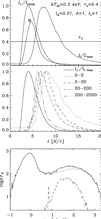
Figure 4: Upper panel: Response of the coronal parameters to a strong dissipation in the corona. The normalised $l_{\mathrm{c}}$ profile defined by Eq. (1) is shown together with the volume averaged temperature, $\theta=kT_{\mathrm{e}}/m_{\mathrm{e}}c^{2}$, response , total optical depth, and the system total luminosity light curve. Middle panel: associated light curves. The profile of the disk dissipation parameter $l_{\mathrm{d}}$ is shown in solid line. Energy bands used are given in keV. All curves are normalised to their maximum. Bottom: Time average spectrum. The primary emission is shown in dotted line, the reflection component in dashed line.

Figure 5: Upper panel: Response of the coronal parameters to a strong dissipation in the corona. The normalised $l_{\mathrm{c}}$ profile defined by Eq. (1) is shown together with the volume averaged temperature, $\theta=kT_{\mathrm{e}}/m_{\mathrm{e}}c^{2}$, response , total optical depth, and the system total luminosity light curve. Middle panel: associated light curves. The profile of the disk dissipation parameter $l_{\mathrm{d}}$ is shown in solid line. Energy bands used are given in keV. All curves are normalised to their maximum. Bottom: Time average spectrum. The primary emission is shown in dotted line, the reflection component in dashed line.

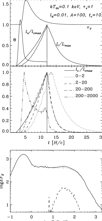
Figure 6: Upper panel: Response of the coronal parameters to a strong dissipation in the corona. The normalised $l_{\mathrm{c}}$ profile defined by Eq. (2) is shown together with the volume averaged temperature, $\theta=kT_{\mathrm{e}}/m_{\mathrm{e}}c^{2}$, and total optical depth response, and the system total luminosity light curve. Middle panel: associated light curves. The profile of the disk dissipation parameter $l_{\mathrm{d}}$ is shown in solid line. Energy bands used are given in keV. All curves are normalised to their maximum. Bottom: Time average spectrum. The primary emission is shown in dotted line, the reflection component in dashed line.

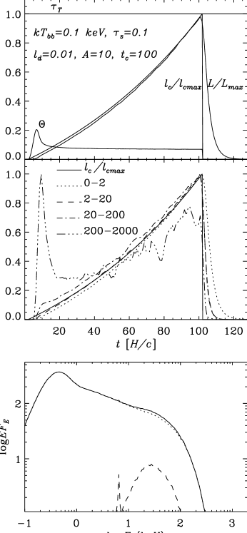
Figure 7: Upper panel: Response of the coronal parameters to a strong dissipation in the corona. The normalised $l_{\mathrm{c}}$ profile defined by Eq. (2) is shown together with the volume averaged temperature, $\theta=kT_{\mathrm{e}}/m_{\mathrm{e}}c^{2}$, and total optical depth response, and the system total luminosity light curve. Middle panel: associated light curves. The profile of the disk dissipation parameter $l_{\mathrm{d}}$ is shown in solid line. Energy bands used are given in keV. All curves are normalised to their maximum. Bottom: Time average spectrum. The primary emission is shown in dotted line, the reflection component in dashed line.

the Schwarschild radius of a 10 $M_{\sun}$ black hole, the light crossing time is $R_{\mathrm{g}}/c=10^{-4}s$. We thus need flare durations which are only one order of magnitude larger than the light crossing time. On the other hand, the invoked dissipation mechanism, magnetic reconnection, is very fast, due to the high speed of Alfvèn waves which approaches the speed of light. The reconnection time could be of a few $H/c$ only. There are thus indications that at least a fraction of the luminosity could be emitted under non-equilibrium conditions.

Let us now consider the case of a short flare in the corona. We assume that the system is initially in a steady state where the corona is not (or almost not) powered. At a given time, a strong dissipation occurs in the corona. We model this flare by increasing abruptly $l_{\mathrm{c}}$. The influence of the temporal profile $l_{\mathrm{c}}(t)$, the characteristic duration and amplitude of the dissipation are then to be studied.

6.2 Results of simulations

As an example, we take the following profile for the temporal dependence of the dissipation parameter:

$$l_{\mathrm{c}}(t) = 0\qquad\mathrm{when}\quad t<2$$

$$l_{\mathrm{c}}(t) = A(t-2)^{2}\exp\left(-\frac{t-2}{t_{\mathrm{c}}}\right)\qquad\mathrm{when}\quad t>2$$ (1)

Fig. 4 shows the coronal parameters response for $A=1$, $t_{\mathrm{c}}=H/c$. At the beginning of the shot the radiative losses are negligible since the photon energy density is very weak. The energy dissipation leads to a quick increase of the coronal temperature.

A higher temperature means higher Compton losses. But as the thermal plasma is still photon-starved, cooling is not efficient and the temperature still increases. However, a high energy photon component forms in the medium. Approximately half of these photons, directed upward escapes. The others travel toward the disk. There, they are instantaneously reprocessed and reinjected in the corona as soft radiation. The radiative energy is conserved through reprocessing. However, a few high energy photons are transformed in numerous soft photons which are able to cool the plasma efficiently. Then the temperature decreases and the escaping photon spectrum softens. This feedback mechanism is delayed in time of a few $H/c$ due to the photon travel time effect. Thus, if the dissipation parameter increases significantly over this time scale, the system cannot adjust gradually and a brutal temperature increase is unavoidable.

The time (and angle) averaged spectrum of the flare is shown in Fig. 4. This spectrum is roughly similar to those we get in stationary situations; however there are some important differences that we have to point out.

The maximum temperature during the flare ($kT_{\mathrm{e,max}}\sim 400$ keV) is about 4 times higher than the allowed maximum temperature in steady situations for a slab geometry. As a consequence the overall averaged spectral shapes differ. In the steady state situation, for optical depth, $\tau_{\mathrm{T}}=0.4$, the equilibrium temperature is only 87 keV, leading to a sharp cut-off in the spectrum above 100 keV. The intrinsic 4-20 keV slope of the angle averaged spectra is then $\Gamma=2.04$. The spectrum shown in Fig 4 has a slightly harder spectral slope $\Gamma=1.89$. It also extends to higher energies than the steady state spectrum does. In the example of Fig. 4 about 9 % of the total luminosity is emitted above 200 keV, while in the steady state case this fraction is only of 2 %.

The associated light curves shown in Fig. 4 exhibit the hard-to-soft spectral evolution of the flare. We can also note the time delay between the light curves and the dissipation profile. This delay is due to photon trapping and multiple reflections in the disk/corona.

The maximum temperature achieved depends mainly on the dissipation amplitude $A$ and characteristic time $t_{\mathrm{c}}$. Higher temperatures are obtained for higher amplitudes and shorter durations. The maximum temperature is also higher when the initial photon energy density is small (i.e. small dissipation parameter $l_{\mathrm{d}}$). By manipulating these parameters one can thus obtain very large temperature jumps. For instance, Fig 5 shows the evolution of the parameters during a flare similar to that of Fig. 4 with the amplitude $A$, however, larger by a factor of 20. The maximum temperature is around 1.5 MeV. At such a high temperature, numerous photons with energy higher than the pair production threshold are produced. Pair production then increases the optical depth by a factor of two. After the end of the dissipation, it takes a few $H/c$ for these pairs to annihilate. This annihilation process leads to the formation of an annihilation line in the average spectrum of the flare (shown in Fig. 5). Note also the high energy tail which extends up to MeV energies. This tail is formed at the beginning of the flare when the temperature is very high. However, due to the important increase of the optical depth during the flare, the 4-20 keV spectral slope is softer ($\Gamma=2.07$) than in the example of Fig. 4.

The light curves presented in Fig 5 are very similar to those of the previous example (Fig. 4). The lag between hard and soft photons is a general feature of the corona where heating is too fast to enable a quasi-static evolution.

This jump in temperature always occurs at the beginning of the dissipation since the soft photon energy density is then minimum. After the bulk of energy has been dissipated, it takes $\sim 10-20H/c$ for it to leave the corona as radiation and for the system to relax.

We can try another shape for the dissipation profile. Fig. 6 shows the evolution of the coronal parameters as a response to a dissipation with exponential rise and instantaneous decay:

$$l_{\mathrm{c}}(t) = 0\qquad\mathrm{when}\quad t<2\qquad{\mathrm{and}}\qquad t>2+t_{\mathrm{c}}$$

$$l_{\mathrm{c}}(t) = A\frac{\mathrm{e}^{(t-2)/t_{\mathrm{c}}}-1}{\mathrm{e}-1}\qquad\mathrm{when}\quad 2<t<2+t_{\mathrm{c}}$$ (2)

The shot amplitude and duration have been fixed respectively at $A=100$ and $t_{\mathrm{c}}=10$ $H/c$. The optical depth associated with ions is $\tau_{\mathrm{s}}=1$. The temperature, after having reached its maximum ($\sim$ 550 keV) at the very beginning of the flare, decreases to its steady state equilibrium value ($\sim$ 50 keV) as the dissipation parameter still rises.

The initial temperature increase leads to an intense pair production raising the optical depth by $\Delta\tau_{\mathrm{T}}=0.6$. The annihilation of the pair excess does not form an annihilation line. Due to the high impulse amplitude, the line emissivity is negligible compared to the continuum high energy flux. Thus a large increase of the optical depth during the flare does not systematically involve the formation of an annihilation line.

The flare light curves are shown in Fig. 6. One can see that the 200-2000 keV light curve reaches its maximum at the very beginning of the shot unlike the lower energy bands which follow the dissipation curve. This peak is obviously linked with the temperature maximum. Here again the spectral evolution leads to soft-photon lags.

If the shot duration is long ($t_{c}\gg 1$), as in the example of Fig. 7 where $A=10$ and $t_{c}=100H/c$, the system is in quasi equilibrium state during 80% of the flare duration. The radiation produced during the initial temperature excess is negligible in the integrated spectrum. This resulting spectrum (shown in Fig. 7) is the same as the one obtained in the steady state approximation. The 4-20 keV slope is $\Gamma=2.33$; it is then interesting to compare this spectrum to that of Fig. 6 which is harder ($\Gamma=2.00$) and presents a high energy tail.

Although it is not a characteristic linked with the dynamics, we can also note that the large optical depth of order unity considered here wipes out the reflection features, reducing the apparent amount of reflection.

6.3 Discussion

Our simulations show that when the dissipation time is short, the spectral evolution during the flare evolves from hard to soft producing soft-photon lags. As expected, a fast dissipation induces a temperature jump at the beginning of the flare, followed by a cooling.

This arises from the response time of the disk due to photon travelling in the corona. The slab corona geometry considered here has the shortest response time. Other geometries where the corona is physically separated from the disk have a longer feedback time. We thus expect this effect to be amplified in such configurations.

Such soft lags are not compatible with hard lags generally observed in X-ray binaries (e.g., Cui 1999 and references therein). Observations, however, generally show hard lags in X-ray binaries only up to 30 Hz. The lags cannot presently be measured at higher frequencies.

If we assume that the size of the corona is of the order of the Schwarschild radius of a 10 $M_{\sun}$ black hole, the light crossing time is $R_{\mathrm{g}}/c=10^{-4}\mathrm{s}$. The observed lags are thus associated with variability on time scales greater than 50 $R_{\mathrm{g}}/c$, probably large enough for a quasi-static evolution to take place.

This low frequency variability could be due to long (quasi-static) independent events, then the observed hard lags would be the consequence of the individual flare spectral evolution which is then quasi-steady. More likely, the low frequency variability could be due to a succession of correlated shorter events (Poutanen & Fabian 1999). The observed time lags would then depend on the spectral evolution of the avalanche and not necessarily on the individual flare spectral evolution.

Each short flare event can then have a hard to soft spectral evolution. The only constraint, in order to be consistent with the observations, is that the flares should be on average softer at the beginning, and harder at the end of the avalanche.

Anyway models where variability is driven by the dissipation in the corona predict that the lags should invert from hard to soft lags at some frequency related to the size of the emitting region. We showed that a dissipation occuring on time scales of $\sim 10H/c$ can produce soft lag while dissipations on time scales $\sim 100H/c$ enable a quasi-steady state evolution. Thus the lag inversion lies somewhere in between these two time scales. If we assume $H/c\sim R_{\mathrm{g}}/c\sim 10^{-4}\mathrm{s}$, then the lag inversion occurs below $\sim 150$ Hz. In other words, the observation of such a lag inversion would put constraints on the size of the emitting region. Detailed Monte-Carlo simulations can help in determining precisely where the lag inversion should fall, depending mainly on geometry.

We can also note that coronal flare heating and subsequent cooling by reprocessing might explain the soft lags observed in neutron star systems such as the millisecond pulsar SAX J1808.4-3658 (Cui et al., 1998) or in the kHz QPO of 4U 1608-52 (Vaughan et al., 1997, 1998).

In addition, we showed that the dynamical processes can also have an influence on the average spectra. As a consequence of the rise in temperature, which reaches higher values than in steady state situations, it is possible to obtain harder spectra. This could relax somewhat the geometry constraints on spectral shape.

With convenient parameters, this thermal model can even produce annihilation lines. The details of the physics of accretion disk coronae are presently unknown. We have thus very few physical constraints, and the parameters required in order to get an annihilation line seem to us plausible. The line appears however for a limited range of parameter values. An intense pair production rate is required at the beginning of the flare and thus a huge dissipation on very short time scales. If, however, the dissipation amplitude is too large the line disappears because of the strong luminosity in the continuum around 511 keV.

The fact that these lines are not observed (see however Bouchet et al. 1991; Goldwurm et al. 1992 ) is consistent with a nearly steady situation in compact sources, but does not imply it.

Another interesting feature is the formation of a high-energy tail at MeV energies. The observed tail in Cyg X-1 (Ling et al. 1997; McConnell et al. 1997) can probably be explained by pure non-equilibrium thermal comptonisation without need for hybrid models.

7 Conclusion

The NLMC method has significantly contributed to the study of the spectral properties of a steady corona radiatively coupled with an accretion disk (e.g. Stern et al. 1995b). However, in order to understand the short term X-ray variability of accreting black hole sources, it seems necessary to take into account the dynamical aspect of the coupling. We have shown that, here again, the NLMC method can be an efficient tool. Our code is able to deal with different situations in which the disk-corona equilibrium is perturbed by a violent energy dissipation in the disk or the corona. The few examples given here are far from being a definitive study of these problems. However, they enable us to outline some important general properties.

On the one hand, we showed that models invoking a variability in the injection of soft seed photons as the origin of hard X-ray variability have to take into account the response of the corona to such fluctuations. Indeed, the corona is quickly Compton cooled when the soft photons flux increases. As long as the coronal heating is kept constant, the whole luminosity of the Comptonised radiation is constant, even if the thermal emission is strongly variable. There is however an important spectral evolution, leading to complex correlations between different energy bands. Details of these correlations depend on the intrinsic soft flux variability.

On the other hand, if the variability arises from dissipation in the corona, the quasi-static approximation is valid as long as the dissipation time scale is far larger than the corona light crossing time. If this is not the case the feedback from the disk leads to a hard-to-soft spectral evolution. Such models thus predict soft lags at high fourier frequencies ($>\sim$ 150 Hz). We also showed that a short dissipation time scale produces harder spectra than steady state dissipation. Moreover, in such conditions, a pure thermal model can produce spectral features such as high-energy tails or annihilation lines which are generally considered as the signature of non-thermal processes.

The present work could be developed in numerous ways. For example, as the disk and corona may be coupled by some physical mechanism, it is likely that the observed variability originates from nearly simultaneous perturbations of the disk and the corona. It is also not very realistic to consider that the dissipation occurs both homogeneously and instantaneously in the corona or the disk: effects of propagation should be introduced. Other complications may arise, such as bulk motions or modifications of the geometry of the emitting region during a flare. The studies of the individual flare evolution should provide predictions for the lag inversion frequencies that can be used to put constraints on the geometry of the sources.

Then, it would be interesting to investigate different stochastic models describing the interaction between flares. Taken together with the evolution of individual flares it would make it possible to generate the light curves in different energy bands, and compute the time-averaged energy spectra and various temporal characteristics such as power spectral density, time/phase lags between different energy bands, cross-correlation functions, coherence function, and compare them with the observations.