Limits of Crystallographic Methods for Detecting Space Topology

Abstract

We investigate to what extent the cosmic crystallographic methods aimed to detect the topology of the universe using catalogues of cosmic objects would be damaged by various observational uncertainties. We find that the topological signature is robust in the case of Euclidean spaces, but is very fragile in the case of compact hyperbolic spaces. Comparing our results to the presently accepted range of values for the curvature parameters, the best hopes for detecting space topology rest on elliptical space models.

Preprint: LPT–ORSAY 00/51; UGVA-DPT 00/05–1082

1 Introduction

The search for the topology of the spatial sections of the universe has made tremendous progress in the past years (see Lachièze–Rey and Luminet (1995) for an introduction to the subject and early references, Luminet and Roukema (1999) and Uzan et al. (1999b) for a review of the late developments). Methods using two–dimensional data sets, such as the cosmic microwave background maps planned to be obtained by the MAP and Planck Surveyor satellite missions, and three–dimensional (3D) data sets, such as galaxy, cluster and quasar surveys with redshifts, have been developped.

Following our previous works (Lehoucq et al. 1996, Lehoucq et al. 1999 and Uzan et al. 1999a), we focus on the topological information that can be extracted from a 3D catalogue of cosmic objects. The key point of all the topology–detecting methods is based on the “topological lens effect”, i.e. on the fact that if the spatial section of the universe has at least one characteristic size smaller than the spatial scale of the catalogue, then one should observe different images of the same object. The original crystallographic method (Lehoucq et al. 1996) used a pair separation histogram (PSH) depicting the number of pairs of catalogue’s objects having the same three–dimensional separations in the universal covering space, with the idea that spikes should stand out dramatically at characteristic lengths related to the size of the fundamental domain and to the holonomies of space. However, following a remark by Weeks (1998), we proved (Uzan et al. 1999a and Lehoucq et al. 1999) that sharp spikes can emerge in the PSH only if the holonomies of space are Clifford translations – a result independently derived by Gomero et al. (1998). As a consequence, the PSH method does not apply to the detection of topology in universes with hyperbolic spatial sections.

Since then, various generalisations of the crystallographic method were proposed. Fagundes and Gaussman (1998) suggested to map the differences between the PSH of a simulated catalogue in a compact hyperbolic universe and the PSH in the corresponding simply–connected universe having the same distribution of objects and cosmological parameters. They noticed sharp oscillations on the scale of the bin width, modulated by a broad oscillation on the scale of the curvature radius. However in Uzan et al. (1999b), we calculated on one hand the differential PSH between a simulated distribution in a compact hyperbolic Weeks space and a similar distribution in the simply–connected hyperbolic space $\bf{H}^{3}$, on the other hand the differential PSH between two different distributions (with the same total number of objects) in the simply–connected hyperbolic space $\bf{H}^{3}$. Both curves (fig. 10 of Uzan et al. 1999b) exhibit the same pattern of sharp and broad oscillations, which shows that the topological significance of such a pattern is highly doubtful.

Fagundes and Gaussman (1999) next proposed a modified crystallographic method in which the topological images in simulated catalogues are pulled back to the fundamental domain before the set of 3D distances is calculated. The distribution of pair distances is expected to be peaked around zero. The main drawback of this method is that the nature of the signal strongly depends on the topological type, on the orientation of the fundamental domain and on the position of the observer inside the latter. Thus the pullback method can be useful only if the exact topology is already known. On the other hand, Gomero et al. (1999) introduced a mean PSH, aimed to reduce the statistical noise that may mask the topological signature. They claimed that such a technique should detect the contribution of non-translational isometries to the topological signal, whatever the curvature of space, but the applicability of their method to real data has not been demonstrated.

In order to improve the signal–to–noise ratio inherent to PSH’s , instead of reducing the statistical noise we can enhance the topological signal by collecting all distance correlations into a single index. Such was our purpose in Uzan et al. 1999a, where we reformulated cosmic crystallography as a collecting-correlated-pairs method (CCP). The CCP technique rests on the basic fact that in a multiply connected universe, equal distances appear more often than just by chance, whatever the curvature of space and the nature of holonomies. We also showed that the extraction of a topological signal drastically depends on the rather accurate knowledge of the cosmological parameters, namely the density parameter, $\Omega_{0}$, and the cosmological constant parameter, $\Omega_{\Lambda 0}$. This is due to the fact that all cosmic crystallography methods require the determination of 3D separations between two any images: observations use redshifts for determining the coordinate distance in the universal covering space (in addition to the angular positions on the celestial sphere), and the redshift–distance relation involves the cosmological parameters. Conversely, the detection of a topological signal would help to determine accurately the curvature parameters (see also Roukema and Luminet 1999).

However it is to be recognized that, in the framework of cosmic crystallography, the application of numerical simulations to real data rest on two idealized assumptions, namely:

1. all objects are strictly comoving

2. the catalogues of observed objects (quasars, galaxy clusters) are complete.

Although quoted in Lachièze–Rey and Luminet (1995), the quantitative effects of such simplifications have not been fully discussed in the literature. In Lehoucq et al. (1996), the authors qualitatively argued that the distortion due to peculiar velocities was negligible, and they performed numerical simulations to study the influence of the angular resolution of the surveys. In Roukema (1996), the influence of the astrophysical uncertainties (mainly of spectroscopic measurements and of peculiar velocities) on a method trying to find quintuplets of quasars with the same geometry (and thus which may be topological images) was evaluated. It was shown that, in such a case, the most serious uncertainty comes from the radial peculiar velocities. In Uzan et al. (1999a), we discussed the effect of the peculiar velocities and of the errors in the spatial position arising from the imprecisions on the values of the cosmological parameters. To finish, the errors on the determination of the position and of the peculiar velocities were discussed in Roukema (1996), and the way that the constraints on $\Omega_{0}$ and $\Omega_{\Lambda 0}$ depend on the redshifts of multiple topological images and on their radial and tangential separations was calculated in Roukema and Luminet (1999).

The goal of the present article is to have a critical attitude on the methods we have developped so far, by listing all the sources of observational uncertainties and by evaluating their effects on the theoretical efficiencies of the PSH method (Lehoucq et al. 1996) and of the CCP method (Uzan et al. 1999a) respectively. In § 2, we discuss the nature of uncertainties and in § 3 the numerical methods used to estimate their effects on the topological signal. We then quantify the magnitude of each effect in the Euclidean and hyperbolic cases (§ 4) (we postpone the case of elliptic spaces to a further study). In conclusion (§ 5) we compare our results to the performances of current and future observational programs aimed to detect the topology of the universe.

Notations and descriptions

We keep the notations of our previous articles (Lehoucq et al. 1999, Uzan et al. 1999a). The local geometry of the universe is described by a Friedmann–Lemaître metric

$${\rm d}s^{2}=-{\rm d}t^{2}+a^{2}(t)\left[{\rm d}\chi^{2}+f^{2}(\chi)\left({\rm d}\vartheta^{2}+\sin^{2}\vartheta{\rm d}\varphi^{2}\right)\right],$$ (1)

where $a$ is the scale factor, $t$ the cosmic time, $\chi$ the comoving radial distance, and $f(\chi)=(\sin\chi,\chi,{\rm sinh}\chi)$ according to the sign of the space curvature $k=(+1,0,-1)$. The time evolution of $a$ is obtained by solving the Friedmann and the conservation equations

$$H^{2} = \kappa\frac{\rho}{3}-\frac{k}{a^{2}}+\frac{\Lambda}{3},$$ (2)

$$\dot{\rho} = -3H(\rho+P)$$ (3)

where $\kappa\equiv 8\pi G/c^{4}$, $\rho$ and $P$ are respectively the matter density and the pressure, $\Lambda$ is the cosmological constant and $H\equiv\dot{a}/a$ is the Hubble parameter (with a dot referring to a time derivative). We also use the standard parameters

$$\Omega\equiv\frac{\kappa\rho}{3H^{2}}\quad\hbox{and}\quad\Omega_{\Lambda}\equiv\frac{\Lambda}{3H^{2}}.$$ (4)

This completely specifies the properties and the dynamics of the universal covering space. In the following, we assume that we are in the matter dominated era, so that $P=0$ and $\rho\propto a^{-3}$.

The topology of the spatial sections is described by the fundamental domain, a polyhedron whose faces are pairwise identified by the elements $g$ of the holonomy group $\Gamma$ (see Lachièze–Rey and Luminet (1995) for the details).

2 Observational uncertainties

Early methods used to put a lower bound on the size of the universe and based on the direct recognition of multiple images of given objects – such as our Galaxy (Sokolov and Schvartsman 1974), the Coma cluster (Gott 1980) – had to face a major drawback due to the fact that the same object would be seen at different lookback times. Thus, evolution effects such as photometric or morphologic changes will, in most cases, render the identification of objects impossible (see however Roukema and Edge, 1997). Statistical techniques such as the PSH method (Lehoucq et al. 1999) and the CCP method (Uzan et al. 1999a) are free from such biases.

The two main sources of uncertainties for all the statistical methods trying to detect the topology of the universe in catalogues of cosmic objects are

1. the errors in the positions of observed objects, which can be separated into:

   1. the uncertainty in the determination of the redshifts due to spectroscopic imprecision; such an effect is purely experimental and exists even if the objects are strictly comoving

   2. the uncertainty in the position due to peculiar velocities of objects, which induce peculiar redshift corrections

   3. the uncertainty in the cosmological parameters, which induces an error in the determination of the radial distance (via the redshift – distance relation)

   4. the angular displacement due to gravitational lensing by large scale structure.

2. the incompleteness of the catalogue, which has two main origins:

   1. selection effects implying that some objects are missing from the catalogue

   2. the partial coverage of the celestial sphere, due either to the presence of the galactic plane, or to the fact that surveys are performed within solid angles much less than $4\pi$.

Effects of peculiar velocities

A peculiar velocity has two effects on the determination of the position of a cosmic object:

1. An integrated effect, coming from the fact that if a galaxy has a proper velocity, then its true position differs from its comoving one.

2. An instantaneous effect, due to the fact that the radial component of the proper velocity will add to the cosmological redshift an extra term, $\Delta z_{Dop}$.

Assuming that the vector velocity $\@vec{v}$ of a galaxy is constant, which is indeed a good enough approximation to estimate the effects of peculiar velocities, a galaxy at redshift $z$ has moved from its comoving position by a comoving distance

$$\delta\@vec{\ell}=\@vec{v}\tau[z]$$ (5)

where $\tau[z]$ is the look–back time, obtained by integrating the photon geodesic equation

$$\tau[z]=\frac{1}{H_{0}}\int_{\frac{1}{1+z}}^{1}\frac{{\rm d}x}{\sqrt{\Omega_{\Lambda 0}x^{2}+(1-\Omega_{0}-\Omega_{\Lambda 0})+\Omega_{0}/x}}.$$ (6)

This reduces to the well known expression

$$\tau[z]=\frac{2}{3H_{0}}\left(1-\frac{1}{(1+z)^{3/2}}\right)$$ (7)

when $\Omega_{0}=1$ and $\Omega_{\Lambda 0}=0$.

Now, $\delta\@vec{\ell}$ can be expressed in terms of a peculiar redshift, $\Delta z_{\rm pos}$, and of an angular displacement, $\Delta\theta_{\rm pos}$, which depend on the galaxy velocity as

$$\Delta z_{\rm pos} = \frac{v_{\parallel}}{c}\frac{c\tau[z]}{\chi^{\prime}[z]}$$ (8)

$$\Delta\theta_{\rm pos} = \frac{|\@vec{v}_{\perp}|}{c}\frac{c\tau[z]}{\chi[z]}$$ (9)

where a prime refers to derivative with respect to $z$, $v_{\parallel}$ is the component of the velocity $\@vec{v}$ with respect to the line–of–sight direction $\@vec{\gamma}$, and $\@vec{v}_{\perp}$ is the non–radial peculiar velocity, defined as

$$v_{\parallel}\equiv\@vec{v}.\@vec{\gamma}\quad\hbox{and}\quad\@vec{v}_{\perp}\equiv\@vec{v}-v_{\parallel}\@vec{\gamma}.$$ (10)

$\chi[z]$ is the observer area distance, given by

$$\chi[z]=\frac{c}{a_{0}H_{0}}\int_{\frac{1}{1+z}}^{1}\frac{{\rm d}x}{\sqrt{\Omega_{\Lambda 0}x^{4}+(1-\Omega_{0}-\Omega_{\Lambda 0})x^{2}+\Omega_{0}x}}.$$ (11)

In figures 1 and 2, we respectively depict the variations of $\Delta z_{\rm pos}$ and $\Delta\theta_{\rm pos}$ as a function of the redshift.

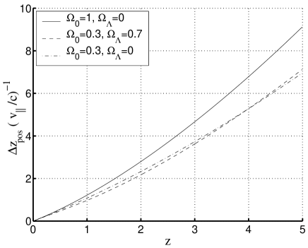
Figure 1: Variation of $\Delta z_{\rm pos}$ in units of $(v_{\parallel}/c)$ as a function of the redshift, assuming the galaxy peculiar velocity is constant.

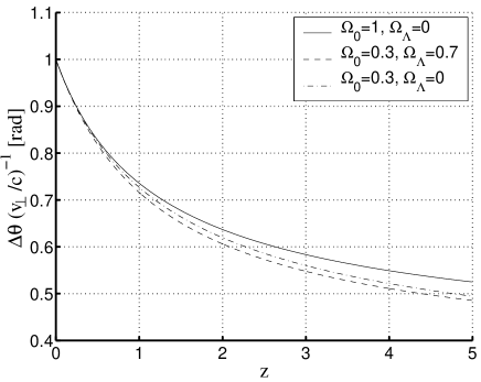
Figure 2: Variation of $\Delta\theta_{\rm pos}$ as a function of the redshift. As long as $z<5$, we have that $\Delta\theta_{\rm pos}/1\,{\rm rad}<0.5(v_{\perp}/c)$. Note also that when $z\rightarrow 0$, $\Delta\theta_{\rm pos}/1\,{\rm rad}\rightarrow(v_{\perp}/c)$.

Concerning the instantaneous effect ii), the redshift uncertainty $\Delta z_{\rm Dop}$ can be related to the galaxy proper velocity as follows.

If we consider the trajectory of a photon $x^{\mu}(s)$, $s$ being the affine parameter along the null geodesic, the relation between the emission (E) wavelength $\lambda_{\rm E}$ and the reception (R) wavelength $\lambda_{\rm R}$ can be expressed as

$$\frac{\lambda_{\rm R}}{\lambda_{\rm E}}=\frac{\left(k^{\mu}u_{\mu}^{\rm obs}\right)_{\rm E}}{\left(k^{\mu}u_{\mu}^{\rm gal}\right)_{\rm R}}$$ (12)

where $k^{\mu}\equiv dx^{\mu}/ds$ is the tangent vector to the photon geodesic; $u_{\mu}^{\rm obs}$ and $u_{\mu}^{\rm gal}$ are respectively the 4–velocity of the observer and of the galaxy. Neglecting the perturbations of the metric and of the matter and focusing on the Doppler effect, one can easily show that

$$k^{\mu}u_{\mu}=-\frac{1}{a(t)}\left[1+\gamma^{i}\frac{v_{i}}{c}\right],$$ (13)

where $\gamma^{i}$ is the direction in which the galaxy is observed and $v^{i}$ is its (Newtonian) velocity. The observed (spectroscopic) redshift, $z_{\rm obs}$, and the cosmological redshift, $z_{\rm cosm}$, respectively defined by

$$1+z_{\rm obs}\equiv\frac{\lambda_{R}}{\lambda_{E}},\quad 1+z_{\rm cosm}\equiv\frac{a(t_{E})}{a(t_{R})}$$ (14)

are thus related by

$$1+z_{\rm obs}=(1+z_{\rm cosm})\left[1+\gamma^{i}\frac{(v_{i}^{\rm gal}-v_{i}^{\rm obs})}{c}\right].$$ (15)

Assuming that we can substract the Earth’s velocity, an error $\Delta z\equiv z_{\rm obs}-z_{\rm cosm}$ in the determination of $z_{\rm obs}$ can be interpreted in terms of a radial peculiar velocity given by

$$\Delta z_{\rm Dop}=\frac{v_{\parallel}^{\rm gal}}{c}(1+z_{\rm cosm}).$$ (16)

As expected, a galaxy receding from us, i.e. with $\gamma^{i}v_{i}^{\rm gal}>0$ will have an additional redshift, whereas a galaxy drawing nearer to us will induce a Doppler blueshift correction.

The considerations above are also useful for discussing the effects of angular displacement $\Delta\theta_{\rm gl}$ due to gravitational lensing by large scale structure (Mellier 1999, van Waerbeke et al. 2000). A typical value $\Delta\theta_{\rm gl}\sim 1$ arcsec corresponds to a peculiar velocity a few km.s^-1 as long as the redshift is less than 5 (as can be seen from Fig. 2). Thus effect $(A4)$ is much less important than effect $(A2)$.

Effects of catalogue incompleteness

Objects can be missing from a catalogue due to strong evolution effects (this is particularly the case for quasars), and to absorption of light by intergalactic gas or dust in some sky directions. Another well known selection effect is the Malmquist bias: statistical samples of astronomical objects which are limited by apparent magnitude have mean absolute magnitudes which are different than those of distance–limited samples. An apparent magnitude–limited sample contains, if luminosity function has a finite width, some very luminous objects which, in spite of their large distances, can jump the apparent-magnitude limit of the catalogue. While one looks further and further out one finds more and more luminous objects. The consequence for an apparent–magnitude catalog (which is the case with galaxy catalogues) is that dwarf galaxies fade out quickly with distance, and finally at the largest distances the extremely luminous and rare galaxies are the only ones which can enter the catalogue.

In addition to effects (B1) and (B2), some noise spikes may appear due to gravitational clustering of objects. The large scale distribution of galaxies shows a variety of landscapes containing voids, walls, filaments and clusters in a complex 3D sponge-like pattern. For instance, since there are many galaxies in clusters, the distances associated to cluster-cluster separations may appear as fake spikes in the PSH for galaxies. Typical cluster – cluster separations are $130h^{-1}$ Mpc (Guzzo et al. 1999). Such effects currently occur in N–body simulations that show clustering (Park and Gott 1991). The trouble can be relieved if galaxy clusters instead of galaxies are used as typical objects for probing the topology, although in that case supercluster-supercluster separations might also introduce noise spikes (at a lower level).

3 Numerical implementation

In the following, we perform numerical simulations to evaluate separately the magnitudes of the effects listed above. As usual, we start from a random distribution of cosmic objects in the fundamental domain. In a first step we generate a complete catalogue of comoving objects by unfolding the distribution in the universal covering space. We refer to this catalogue as the ideal catalogue since it would correspond to ideal observations. In a second step we introduce the various errors $(A_{i})-(B_{i})$ in order to build more realistic catalogues which depart from the ideal one.

3.1 Uncertainties on positions

To study numerically the errors on the positions, we first assume that the cosmological parameters are known with good enough accuracy, so that we do not discuss (A3). Then we perform the following calculations.

1. To evaluate the effect of the observational imprecision, we give to each object of the ideal catalogue (built on the assumption that the objects are strictly comoving) a redshift error to be added to its ideal redshift. We assume that the distribution of the redshift error is Gaussian, with mean value $\bar{z}=0$ and dispersion $\Delta z$.

   Note that, since $\Delta z$ is absolute, the relative error will be less important when we deal with catalogues of higher redshift objects.

2. To discuss (A2), we associate a peculiar velocity to each point of the catalogue before unfolding. Hence, there will be correlations between the velocities of two topological images. It follows that, assuming that the time evolution of the peculiar velocity is small, the observed velocities of two topological images of the same object can have different directions but similar magnitudes (see e.g. Roukema and Bajtlik 1999). As in the previous case, we assume that the velocity distribution is Gaussian. Moreover, velocities at different points of space are assumed to be uncorrelated both in magnitude and direction, which is indeed not strictly the case in real data since large scale streaming motions of galaxies have been observed (Strauss and Willick 1995).

More precisely, to generate the catalog of topological images taking into account the peculiar velocities, we proceed as follows:

1. We generate a random collection of points $M_{i}$ (named original sources) uniformly distributed inside the fundamental domain. Each point is assigned a velocity $v_{i}$ according to a Gaussian distribution with mean $\bar{v}$ and dispersion $\Delta v$.

2. We unfold this catalogue of original sources to obtain the set of points $M_{k,i}$, images of $M_{i}$ by the holonomies $g_{k}\in\Gamma$.

3. Each image $M_{k,i}$ has a redshift $z_{k,i}$ corresponding to a look–back time $\tau_{k,i}\equiv\tau(z_{k,i})$ calculated with formula (6).

4. The final catalogue accounting for the peculiar velocities of the original sources is obtained by applying the $g_{k}$ to $M_{i}+v_{i}\times\tau_{k,i}$ for all couples $(k,i)$.

Since $\Delta z$ can be interpreted either as an uncertainty on the redshift determination or as due to a radial peculiar velocity, both errors (A1) and (A2) can be investigated with the same calculations. The interpretation of $\Delta z$ in terms of a radial peculiar velocity is useful to compare the orders of magnitude of (A1) and (A2). In real data, the error due to (A2) is expected to be greater than the error due to (A1).

3.2 Catalogue incompleteness

Starting from an ideal catalogue, we simulate two kinds of incomplete catalogues:

1. To account for effect (B1), we randomly throw out $p\%$ of the objects from the ideal catalogue. In our various runs we vary $p$ while keeping approximately constant the number of catalogue objects, which means that we must increase the number of “original” objects in the fundamental domain when $p$ is increasing.

2. To simulate effect (B2), we generate a catalogue limited in solid angle by selecting only the objects that lie in a beam of aperture $\theta$. The sky coverage is related to $\theta$ via

   $$q\%=\frac{1}{2}\left(1-\cos(\theta/2)\right).$$ (17)

   Again, we keep constant the number of objects in the catalogue when we vary $\theta$. Table 1 below gives typical numbers.

Table 1: The multiplication factor, i.e. the ratio between the total number of entries in the catalogue and the number of “original” objects randomly distributed in the fundamental domain, is given as a function of the solid angle of the survey. We have also indicated the corresponding sky coverage.

$\theta$	multiplication factor	sky coverage ($q$%)
160o	6.75	41.3
80o	1.92	11.7
70o	1.45	9.0
60o	1.06	6.7

As a matter of fact, more than the aperture angle, the depth of the survey will be critical for the multiplication factor, since within a beam of given angle, if the redshift cut-off is great enough to encompass a distance (in the universal covering space) N times greater than the size of the fundamental domain, at least N topological images will be expected in the beam.

4 General Results

4.1 Euclidean spaces

We first consider the Euclidean case and we apply the PSH crystallographic method as described in Lehoucq et al. (1996), restricting to a typical situation where $\Omega_{0}=0.3$ and $\Omega_{\Lambda 0}=0.7$. We choose the topology of the universe to be a cubic 3–torus $T_{1}$ (see e.g. Lachièze–Rey and Luminet (1995) for description), with identification length $L=3,000\,{\rm Mpc}$ for a Hubble parameter $H_{0}=75\,{\rm km.s}^{-1}{\rm Mpc}^{-1}$. In the various runs, the number of objects in the catalogue is kept constant at $8500$ (this is the order of magnitude of the number of objects in current quasar catalogues). We examine separately the effects of errors in position due to redshift uncertainty $\Delta z$ and peculiar velocities $\Delta v$, and the effects of catalogue incompleteness due to selection effects and partial sky coverage. Each of these effects will contribute to spoil the sharpness of the topological signal. For a given depth of the catalogue, namely a redshift cut-off $z_{cut}$, we perform the runs to look for the critical value of the error at which the topological signal fades out.

Figure 3 gives the critical redshift error $\Delta z_{l}$ above which the topological spikes disappear.

Figure 3: Plot of $\Delta z_{l}$ as a function of the depth of the catalogue, for a cubic hypertorus of size $3,000$ Mpc which corresponds to 45% of the Hubble radius ($4,950\,h^{-1}$ Mpc) when $\Omega_{0}=0.3$, $\Omega_{\Lambda 0}=0.7$ and $h=0.75$, using the PSH method.

The effect of peculiar velocities is very weak, since we find that the peculiar velocity must exceed $\Delta v_{l}=10,000\,{\rm km.s}^{-1}$ when $z_{cut}=1$ and $\Delta v_{l}=40,000\,{\rm km.s}^{-1}$ when $z_{cut}=5$ in order to make the topological signal disappear. As already pointed out in Lachièze–Rey and Luminet (1995), the observed peculiar velocities of galaxies have typical values much less that $\Delta v_{l}$.

The effects of catalogue incompleteness are summarized in tables 2 and 3. The topological signal would be destroyed only for a very large rejection percentage or a small aperture angle.

Table 2: Values of the critical percentage of rejection above which the PSH spikes disappear, as a function of the redshift cut–off.

$z_{\rm cut}$	$\qquad 1\qquad$	$\qquad 2\qquad$	$\qquad\geq 3\qquad$
$p_{l}[\%]$	$\qquad 70\qquad$	$\qquad 80\qquad$	$\qquad>90\qquad$

Table 3: Values of the aperture angle below which the PSH spikes disappear, as a function of the redshift cut–off.

$z_{\rm cut}$	$\qquad 2\qquad$	$\qquad 3\qquad$	$\qquad 4\qquad$	$\qquad 5\qquad$
$\theta_{l}$	$\qquad 110^{\rm o}\qquad$	$\qquad 80^{\rm o}\qquad$	$\qquad 70^{\rm o}\qquad$	$\qquad 60^{\rm o}\qquad$

4.2 Hyperbolic spaces

We now turn to universes with hyperbolic spatial sections and apply the CCP method as described in Uzan et al. (1999a). The obtention of a topological signal (the so–called CCP index) strongly depends on the correct determination of the cosmological parameters. In Uzan et al. (1999a) we discussed the problems arising from the spanning of the cosmological parameters space with a required “accuracy bin” $\varepsilon$. Latest independent constraints on these cosmological parameters from the cosmic microwave background (de Bernardis et al. 2000), the study of supernovae (Efstathiou et al. 1999), of large scale structure at $z=2$ (Roukema and Mamon, 2000) and of gravitational lensing (Mellier 1999), make us hope that we can restrict further the parameters space to apply efficiently the CCP method. In the following, we assume that the cosmological parameters are known with the required accuracy.

We choose the topology of the universe to be described by a Weeks manifold (Weeks, 1985) (see also Lehoucq et al. (1999) for the numerical implementation of this topology), assuming the cosmological parameters given by $\Omega_{0}=0.3$ and $\Omega_{\Lambda 0}=0$. In such a case the number of copies of the fundamental domain within the horizon is about 190. However our simulated catalogues are much smaller than the horizon volume. We fix the number of objects to $1300$, which is a compromise between a realistic catalogue population and a reasonable computing time.

Again we perform the tests by varying the errors $\Delta z$ and $\Delta v$ around their average values $\bar{z}=0$ and $\bar{v}=0$ until when the CCP index falls down to noise level.

Contrarily to the Euclidean case, both slight changes in redshift and in peculiar velocity induce errors in position which dramatically eradicate the topological signal: an error of only $\sim 50\,{\rm kms}^{-1}$ in velocity and an error in redshift of the order of the bin accuracy $\varepsilon\sim 10^{-6}$ drown the CCP index into noise.

The incompleteness effects are less dramatic, as shown in figures 4 and 5. Again, for a given redshift cut–off, we performed the runs by varying $p$ and $\theta$ in order to find the critical values at which the topological signal disappears.

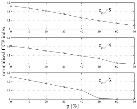
Figure 4: Plot of the CCP–index (normalized to background noise) as a function of the rejection percentage of objects $p_{l}$, for various values of of the depth of the catalogue. The topological signal disappears when the rejection percentage is greater than $p_{l}$.

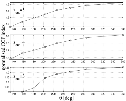
Figure 5: Plot of the CCP–index as a function of $\theta_{l}$ for various values of the depth of the catalogue. The topological signal disappears when the aperture angle falls down below $\theta_{l}$.

5 Conclusions and perspectives

Our numerical results have now to be compared with the precisions of present experimental 3D data, and to the performances of observational programs started or expected to be achieved in the next decade.

At present day, a typical precision practical for the spectroscopic uncertainty is $\Delta z\sim 0.001$ for an object such as a quasar. In clusters, spectroscopic redshifts can be found very precisely for individual galaxies.

Concerning peculiar velocities, the typical dispersion velocity is $1000\,\mathrm{km.s}^{-1}$ in rich clusters. The X-ray velocity of the peak of the X-ray distribution would also provide a way to estimate the true cluster redshift, including the peculiar velocity of the cluster as a whole. For a quasar, a conservative upper limit to the peculiar velocity, assuming the quasar to be at the centre of a galaxy, can be taken as $\Delta z\sim 0.002$. So, from an experimental point of view, the uncertainties on the redshifts will be dominated by effect (A2), namely the peculiar velocities, rather than by the spectroscopic imprecision.

The main limitation of present 3D samples is the small volume of existing redshift data. Future surveys will significantly improve both the redshift cut–off and the sky coverage. For instance, the Sloan Digital Sky Survey (SDSS) (Loveday 1998) will map in detail one-quarter of the entire sky, determining the positions and absolute brightnesses of more than 100 million celestial objects. It will also measure distances to more than a million galaxies and quasars. More precisely, SDSS will map a contiguous $\pi$ steradians area in the north Galactic cap, up to a limiting magnitude 23 for two thirds of the observing time, together with three southern stripes centred at RA $\alpha=5^{\circ}$ and with central declinations of $\delta=+15^{\circ},0^{\circ}$ and $-10^{\circ}$ for the remaining one third of the time. Concerning the distance determinations, $10^{6}$ galaxies and $10^{5}$ quasars will be observed spectroscopically with a resolution $\Delta z/z\sim 5.10^{-4}$. The main galaxy sample will consist of $\sim 900,000$ galaxies up to magnitude 18, with a median redshift $z\sim 0.1$. A second galaxy sample will consist in $\sim 100,000$ luminous red galaxies to magnitude 19.5 with a median redshift $z\sim 0.5$. Precision on redshifts can be estimated for the reddest galaxies to $\Delta z\sim 0.02$. A sample of $\sim 100,000$ quasars will be observed, an order of magnitude larger than any existing quasar catalogue. The complete survey data will become public by 2005. We can also mention the ESO–VLT Virmos Deep Survey Project (Lefèvre 2000), a comprehensive imaging and redshift survey of the deep universe based on more than 150 000 redshifts.

In the field of X–ray observations, the XMM satellite (Arnaud 1996) will provide deep insight on X–ray galaxy clusters and active galactic nuclei. Also, the XEUS project under study by ESA (Parmar et al. 1999) will be a long–term X–ray observatory at 1 keV, with a limiting sensitivity around 250 times better than XMM, allowing XEUS to study the properties of galaxy groups at $z=2$ and active galactic nuclei at $z\lesssim 3$.

In the present paper we have investigated how the various observational uncertainties will spoil the topological signal expected to arise in the ideal situation when crystallographic methods are applied to complete catalogues of perfectly comoving objets with zero proper velocities and whose 3D–positions are known with infinite accuracy. By numerical simulations we have introduced random errors for each possible uncertainty, and we varied the parameters to determine the limits at which the topological signal vanishes.

Our numerical calculations of the spoiling effects due to the various uncertainties $(A_{i})-(B_{i})$ clearly show that the crystallographic methods are stable (in the sense that the topological signal is robust when data depart from the ideal ones) in the Euclidean case, but highly unstable in the hyperbolic case. Indeed in a small multi–connected flat space, realistic values of peculiar velocities of objects, errors in redshift determinations and partial sky coverage will not make the PSH method to fail. This can be understood by the fact that the topological images of a given object are related together by Clifford translations which enhance the topological signal. On the contrary, in a compact hyperbolic model, holonomies are not Clifford translations. The topological signal, built as a CCP index, is destroyed as soon as small errors are introduced in the position of objects, due either to peculiar velocities or to redshift measurement imprecision.

The same kind of critical analysis should be made with the 2D topology–detecting methods based on the analysis of CMB data. For instance, in the pairs of matched circles method (Cornish et al. 1998), it would be necessary to investigate how deviations to the ideal situation, such as a non zero thickness of the last scattering surface or peculiar motions of the emitting primordial plasma regions, would alter the pattern of perfectly matched circles.

To conclude, let us comment on the future of observational cosmic topology, at the light of observational constraints on the curvature parameters recently provided by BOOMERanG and MAXIMA balloon measurements (de Bernardis et al. 2000, Hanany et al. 2000). Under specific assumptions such as a cold dark matter model and a primordial density fluctuation power spectrum, the range of values allowed for the energy-density parameter $\Omega=\Omega_{0}+\Omega_{\Lambda 0}$ is restricted to $0.88<\Omega<1.12$ with $95\%$ confidence. This means that the curvature radius of space is as least as great as the radius of the observable universe (delimited by the last scattering surface). Such results, if accepted, leave open all three cases of space curvature as well as most of multi–connected topologies.

A strictly flat space is quite improbable. Even inflationary scenarios predict a value of $\Omega$ asymptocally close to 1, but not strictly equal. From a topological point of view, a strictly Euclidean space would be interesting since we have shown that the PSH method is robust enough to provide a topological signal even when realistic uncertainties on the data are taken into account.

For compact hyperbolic spaces, if we accept the recent observational constraints $0.88<\Omega_{0}+\Omega_{\Lambda 0}<1$, a number of spaceforms such as the Weeks or the Thurston manifolds still have topological lengths smaller than the horizon size (Weeks: SnapPea). However the topological lens effects would be weaker in spaceforms with $\Omega$ close to 1 than in spaceforms with $\Omega\sim 0.3$ (see figs. 2 and 3 of Lehoucq et al. 1999). Furthermore, only the CCP method can be applied for detecting the topology, and the present article shows that the topological signal will fall to noise level as soon as uncertainties smaller than the experimental ones are taken into account in the simulations.

Eventually, elliptical spaceforms appear to be the most interesting case. On a theoretical point of view, as far as we know, no inflationary model is able to drive the density parameter to a value greater than 1, so that if space happened to be really elliptical, new models should be built in order to explain, e.g., the primordial fluctuations spectrum or the horizon problem. From a topological point of view, since the volumes of (all closed) spaceforms are not bounded below (the order of the holonomy group can be arbitrarily large), one can always find an elliptical space which fits into the Hubble radius even if $1<\Omega_{0}+\Omega_{\Lambda 0}<1.12$. On the other hand, the holonomies of such spaces are Clifford translations, so that we can hope to apply the robust PSH method to detect a topological signal. This will be the purpose of our subsequent paper.

Acknowledgements: It is a pleasure to thank N. Aghanim, R. Juszkiewicz, Y. Mellier and B. Roukema for discussions.

References

- (1) M. Arnaud, 1996, J.A.F. 52 26.
- (2) P. de Bernardis et al., 2000, Nature, 404 955.
- (3) N. Cornish, D. Spergel and G. Starkman, 1998, Class. Quant. Grav. 15 (1998) 2657.
- (4) G. Efstathiou, S.L. Bridle, A.N. Lasenby, M.P. Hobson and R.S. Ellis, 1998, [astro-ph/9812226].
- (5) H.V. Fagundes and E. Gaussman, 1998, [astro-ph/9811368].
- (6) H.V. Fagundes and E. Gaussman, 1999, Phys. Lett. A261 235.
- (7) G.I. Gomero, A.F.F. Teixeira, M.J. Rebouças and A. Bernui, 1998, [gr-qc/9811038].
- (8) G.I. Gomero, M.J. Rebouças and A.F.F. Teixeira, 1999 [astro-ph/9909078]; ibid, [astro-ph/9911049].
- (9) J.R. Gott III, Month. Not. R. Astron. Soc., 1980, 193 153.
- (10) L. Guzzo, 1999, Proc. of the XIXth Texas meeting, Paris 14–18 december 1998, Eds. E. Aubourg, T. Montmerle, J. Paul and P. Peter, [astro-ph/9911115]
- (11) S. Hanany et al., 2000, [astro-ph/0005123].
- (12) M. Lachièze-Rey and J.-P. Luminet, 1995 Phys. Rep. 254 (1995) 135.
- (13) O. Lefèvre, in Clustering at high redshift, 1996, ASP Conference Series, Mazure A. et al. (eds.) (in press) [astro-ph/9605028].
- (14) R. Lehoucq, M. Lachièze-Rey and J-P. Luminet, 1996, Astron. Astrophys. 313 339.
- (15) R. Lehoucq, J-P. Luminet and J-P. Uzan, 1999, Astron. Astrophys. 344 735.
- (16) J. Loveday, 1998, in Dwarf Galaxies and Cosmology, Thuan T.X. et al. (eds.), Editions Frontières, Gif sur Yvette, France.
- (17) J-P. Luminet and B.F. Roukema, 1999, in Theoretical and Observational Cosmology, M. Lachièze-Rey (Ed.), Kluwer Ac. Pub., pp.117-157.
- (18) Y. Mellier, 1999, Ann. Rev. Astron. Astrophys. 37 127.
- (19) A.N. Parmar et al., 1999, [astro-ph/9911494].
- (20) C. Park and J.R. Gott III, 1991, Month. Not. R. Astron. Soc. 249 288.
- (21) B.F. Roukema, 1996, Month. Not. R. Astron. Soc. 283 1147.
- (22) B.F. Roukema and A.C. Edge, 1997, Mon. Not. R. Astron. Soc. 292 105.
- (23) B.F. Roukema and J-P. Luminet, 1999, Astron. Astrophys. 348 8.
- (24) B.F. Roukema and S. Bajtlik, 1999, Mon. Not. R. Astron. Soc. 308 309.
- (25) B.F. Roukema and G. A. Mamon, 2000, Astron. Astrophys. (to appear) [astro-ph/9911413].
- (26) D.D Sokolov and V.F. Schvartsman, 1974, Sov. Phys. JETP 39 196.
- (27) M.A. Strauss and J.A. Willick, 1995, Phys. Rep. 261 271.
- (28) J-P. Uzan, R. Lehoucq and J-P. Luminet, 1999a, Astron. Astrophys. 351 766.
- (29) J-P. Uzan, R. Lehoucq and J-P. Luminet, 1999b Proc. of the XIXth Texas meeting, Paris 14–18 december 1998, Eds. E. Aubourg, T. Montmerle, J. Paul and P. Peter, article no 04/25.
- (30) L. van Waerbeke et al., 2000, Astron. Astrophys. (to appear) [astro-ph/0002500].
- (31) J. Weeks, 1985, PhD. thesis, Princeton University.
- (32) J. Weeks, 1998, private communication.
- (33) J. Weeks : Snappea program http://www.geom.umn.edu:80/software.