Epochs of Maximum Light and Bolometric Light Curves of Type Ia Supernovae

Abstract

We present empirical fits to the $\mathit{UBVRI}$ light curves of type Ia supernovae. These fits are used to objectively evaluate light curve parameters. We find that the relative times of maximum light in the filter passbands are very similar for most objects. Surprisingly the maximum at longer wavelengths is reached earlier than in the $\mathit{B}$ and $\mathit{V}$ light curves. This clearly demonstrates the complicated nature of the supernova emission.

Bolometric light curves for a small sample of well-observed SNe Ia are constructed by integration over the optical filters. In most objects a plateau or inflection is observed in the light curve about 20$-$40 days after bolometric maximum. The strength of this plateau varies considerably among the individual objects in the sample. Furthermore the rise times show a range of several days for the few objects which have observations early enough for such an analysis. On the other hand, the decline rate between 50 and 80 days past maximum is remarkably similar for all objects, with the notable exception of SN 1991bg. The similar late decline rates for the supernovae indicate that the energy release at late times is very uniform; the differences at early times is likely due to the radiation diffusing out of the ejecta.

With the exception of SN 1991bg, the range of absolute bolometric luminosities of SNe Ia is found to be at least a factor of 2.5. The nickel masses derived from this estimate range from 0.4 to 1.1 $M_{\sun}$. It seems impossible to explain such a mass range by a single explosion mechanism, especially since the rate of $\gamma-$ray escape at late phases seems to be very uniform.

1 Introduction

The temporal evolution of a supernova’s luminosity contains important information on the physical processes driving the explosion. The peak luminosity of a Type Ia Supernova (SN Ia) is directly linked to the amount of radioactive $\@element[56]{\mathrm{Ni}}$ produced in the explosion (Arnett et al. arn85 (1985), Branch & Tammann bra92 (1992), Höflich et al. hoe97 (1997), Eastman eas97 (1997), Pinto & Eastman 2000a ). The rise time of the light curve is determined primarily by the explosion energy and the manner in which the ejecta become optically thin to thermalized radiation, i.e. the opacity (Khokhlov et al. kho93 (1993)). The late decline of the light curve is governed by the combination of the energy input by the radioactive material and the rate at which this input energy is converted to optical photons in the ejecta (Leibundgut & Pinto lei92 (1992)).

The apparent uniformity of SN Ia light curves in photographic (pg), $\mathit{B}$, and $\mathit{V}$ filters (Minkowski min64 (1964)) prompted the adoption of standard light curve templates (e.g. Elias et al. eli85 (1985), Doggett & Branch dog85 (1985), Leibundgut et al. 1991b , Schlegel schle95 (1995)). Early indications that the standard templates fail to describe the full range of SN Ia light curves came from the observations of SN 1986G, which displayed a much more rapid evolution than any other SN observed up to that time (Phillips et al. phi87 (1987)). The demise of the simple standard candle treatment was brought about by the observations of the faint SN 1991bg (Filippenko et al. fil92a (1992), Leibundgut et al. lei93 (1993), Turatto et al. tur96a (1996)) and the subsequent derivation of a correlation between peak luminosity and decline rate after maximum (Phillips phi93 (1993), Hamuy et al. 1996a , Riess et al. 1996a ). A clear demonstration that SNe Ia do not display a uniform photometric evolution was provided earlier from the infrared $\mathit{J}$, $\mathit{H}$, and $\mathit{K}$ light curves (Elias et al. eli85 (1985), Frogel et al. fro87 (1987)). Observations and analyses of the near-IR $\mathit{R}$ and $\mathit{I}$ light curves (Suntzeff sun96 (1996), Vacca & Leibundgut vac97 (1997)) confirm this variation. The red and near-infrared light curves exhibit a second maximum $\sim$ 20 to 30 days after the $\mathit{B}$ peak. This second maximum occurs at different phases and with differing strengths in individual SNe Ia and in at least one case (SN 1991bg; Filippenko et al. fil92a (1992), Leibundgut et al. lei93 (1993), Turatto et al. tur96a (1996)) is altogether absent.

The light curves of SNe Ia are often described as a one-parameter family. The correlation of the $\mathit{BVRI}$ light curve shapes with the peak absolute magnitudes has been employed to improve the distance measurements derived from SNe Ia (Hamuy et al. 1996a , Riess et al. 1996a , Garnavich et al. gar98 (1998), Schmidt et al. sch98 (1998), Riess et al. 1998a ) and is of fundamental importance to keep the systematic uncertainties in the derivation of cosmological parameters small. Techniques that fit standard templates (e.g., Hamuy et al. 1996a ), or modified versions of these templates (e.g., Riess et al. 1996a ; Perlmutter et al. per97 (1997)), to the observed light curves make use of this one parameter description of the light curves. These methods have the advantage that they can be applied even to rather sparsely sampled light curves. In a more extreme form, the photometry can be supplemented by spectroscopy to provide a distance measurement with minimal data coverage. This “snapshot” method has been advocated by Riess et al. (1998b ). All these methods make the assumption that SNe Ia form an “ordered class”. This description is validated by the improvement in the scatter around the linear expansion line in the local Universe and also by the fact that new objects can be successfully corrected with the correlations derived from an independent sample.

While clearly useful for comparing local SNe with high redshift SNe, the template method does not allow one to investigate finer and more individual features in a large sample of SN Ia light curves. Hence, the detailed study of the explosion and radiation physics cannot be carried out with such an analysis. For data sets which are densely sampled, however, template methods are not necessary. Recent bright SNe Ia have been observed extensively and very detailed, and accurate light curves have become available. Most of these supernovae have been used as the defining objects for the templates to correct other, more sparsely observed, SNe Ia.

To analyze light curves of many SNe Ia in an individual fashion a parameter fitting method which can be applied to single filter light curves has been devised (Vacca & Leibundgut vac96 (1996, 1997)). The photometric data are approximated by a smooth fitting function. We are not fitting model light curves based on explosion physics, but simply attempt to match the data in an objective way. We have investigated well-observed SNe in a small sample to check our method. It allows us to search for correlations among various light curve parameters, to accurately fit the filter light curves at any phase, and to construct continuous bolometric light curves. The application to the light curves of SN 1994D has already provided one of the first bolometric light curves of SNe Ia (Vacca & Leibundgut vac96 (1996)).

Observationally-derived bolometric light curves provide a measure of the total output of converted radiation of SNe Ia, and therefore serve as a crucial link to theoretical models and calculations of SN explosions and evolution. The total luminosity from a SN Ia is much easier to calculate from theoretical models than the individual filter light curves, which are dominated by line blending effects requiring complicated multi-group calculations (Leibundgut & Pinto lei92 (1992), Eastman eas97 (1997), Höflich et al. hoe97 (1997)). In addition, the observed bolometric peak luminosity of SNe Ia provides a measure of the total amount of nickel synthesized in the explosion and can be used to test various explosion models. Although no SN Ia has ever been observed in every region of the electromagnetic spectrum simultaneously, fortunately bolometric light curves can be constructed almost entirely from optical data alone (Suntzeff sun96 (1996), Leibundgut lei96a (1996)).

In Sect. 2 we describe the sample of objects and the data set used. The parameter fitting method employed for our analysis is described in Sect. 3. This is followed by a discussion of the phases of the maximum epoch in different filters (Sect. 4). The construction of the bolometric light curves is presented in Sect. 5 followed by a discussion of the uncertainties in the bolometric light curves. We summarize our findings in Sect. 6; our conclusions are given in Sect. 7.

2 Observational Data

The data for our analysis come from recent photometric observations of bright SNe Ia, consisting of the large data collections presented by Hamuy et al. (1996b ) and Riess (rie96c (1996), see also Riess et al. rie99 (1999)). Table 1 summarizes the objects which have sufficient data, in at least the $\mathit{BVRI}$ filters, to construct accurate individual filter light curves. Listed are the available filters (column 2) and the references of the SN photometry (column 3), the adopted distance modulus (column 4) and its source (column 5). The distance modulus is taken either from direct distance measurements via cepheids, surface brightness fluctuations or Tully-Fisher luminosity–line width relation or by adopting a $H_{0}$ of 65 km s^-1 Mpc^-1 for galaxies in the Hubble flow ($v>2500$ km s^-1). We use the host galaxy dust extinction values of Phillips et al. (phi99 (1999)) (column 6). The Galactic extinction given by the COBE dust maps is provided in column 7 (Schlegel et al. schle98 (1998)).

Not all objects have sufficient observations in all filters to guarantee that our method will work. In some cases, the light curve fits had to be restricted to a limited phase range. Only three objects (SN 1989B, SN 1991T, and SN 1994D) have a significant number of $\mathit{U}$ filter observations. Our analysis does not include any $\mathit{JHK}$ or ultraviolet data.

Table 1: Photometry of well-observed SN Ia

SN	Filter	ref.a	DM	ref.a	$\mathit{E(B-V)}$host	$\mathit{E(B-V)}$gal
					Phillips et al. (phi99 (1999))	Schlegel et al. (sch98 (1998))
(1)	(2)	(3)	(4)	(5)	(6)	(8)
SN1989B	$\mathit{UBVRI}$	1	30.22	14	0.340	0.032
SN1991T	$\mathit{UBVRI}$	2	31.07	15	0.140	0.022
SN1991bg	$\mathit{BVRI}$	3, 4, 5	31.26	16	0.030	0.040
SN1992A	$\mathit{BVRI}$	6	31.34	17	0.000	0.017
SN1992bc	$\mathit{BVRI}$	7	34.82	7	0.000	0.022
SN1992bo	$\mathit{BVRI}$	7	34.63	7	0.000	0.027
SN1994D	$\mathit{UBVRI}$	8, 9, 10, 11	30.68	9	0.000	0.022
SN1994ae	$\mathit{BVRI}$	12	31.86	18	0.120	0.031
SN1995D	$\mathit{BVRI}$	12, 13	32.71	12	0.040	0.058
aReferences:
1 - Wells et al. wel94 (1994), 2 - Lira et al. lir98 (1998), 3 - Filippenko et al. fil92a (1992),
4 - Leibundgut et al. lei93 (1993), 5 - Turatto et al. tur96a (1996), 6 - Suntzeff sun96 (1996),
7 - Hamuy et al. 1996b , 8 - Richmond et al. ric95 (1995), 9 - Patat et al. pat96 (1996),
10 - Meikle et al. mei96 (1996), 11 - Smith et al. priv. comm., 12 - Riess et al. rie99 (1999),
13 - Sadakane et al. sad96 (1996), 14 - Saha et al. sah99 (1999), 15 - Fisher et al. fis99 (1999),
16 - Hamuy et al. 1996a and references therein, 17 - Suntzeff et al. sun99 (1999) and references therein,
18 - Riess et al. 1996a and references therein

3 Fitting filter light curves

3.1 Method

The light curves are analyzed using a descriptive model (Vacca & Leibundgut vac96 (1996)). For each supernova the observed light curve in each filter is fit with an empirical model consisting of a Gaussian (for the peak phase) atop a linear decay (late-time decline), a second Gaussian (to model the secondary maximum in the $\mathit{V}$, $\mathit{R}$, and $\mathit{I}$ band light curves), and an exponentially rising function (for the pre-maximum segment). The functional form of the fit is:

$$m=\frac{f_{0}+\gamma(t-t_{0})+g_{0}\exp\left({\frac{-(t-t_{0})^{2}}{2\sigma_{0}^{2}}}\right)+g_{1}\exp\left({\frac{-(t-t_{1})^{2}}{2\sigma_{1}^{2}}}\right)}{1-\exp\left({\frac{\tau-t}{\theta}}\right)}$$ (1)

The first Gaussian and the decline are normalized to the phase $t_{0}$, while the second Gaussian occurs at a later phase $t_{1}$. The exponential cutoff function for the rise has a characteristic time $\theta$ and a separate phase zero-point $\tau$. The amplitudes of the two Gaussians, $g_{0}$ and $g_{1}$, as well as the intercept of the line, $f_{0}$, the slope, $\gamma$, the phases $t_{0}$ and $t_{1}$, and the widths, $\sigma_{0}$ and $\sigma_{1}$, the characteristic rise time $\theta$ and its phase $\tau$ are free parameters in the fit. Each filter light curve is fitted individually and independently using a $\chi^{2}$-minimization procedure to determine the best-fit values of the parameters. Other parameters which characterize the shape of the light curve, such as the time of maximum brightness or $\Delta m_{15}$, can then be derived from the best-fit model. Although the model is a completely empirical description of the general shape of SNe Ia light curves, we note that theoretical models (Pinto & Eastman 2000a ) predict a Gaussian shape for the peak in models with constant opacity and $\@element[56]{\mathrm{Ni}}$ buried well within the ejecta.

Fig. 1 shows the example of the fit to the $\mathit{R}$ light curve of SN 1992bc.

Figure 1: Fit of Eq. (1) to the $\mathit{R}$ photometry of SN 1992bc. The various components of the fit are displayed as the following: a linear (in magnitudes) decay (dotted line), an exponential rise factor (solid line) from 0 to 1 as indicated by the right ordinate, two Gaussians for the peak and the second maximum (dashed and dashed-dotted line) with the amplitude in magnitudes as indicated by the right ordinate. The inset shows the light curve around maximum light. $\Delta m_{15}$ can be obtained easily because of the continuous representation of the data by the fit. The residuals from the fit are displayed in the bottom panel with the observational error bars.

The various components of the fit are displayed. The exponential function (solid line) rises steeply to unity, modeling the rapid brightness increase of the supernova. The decline rate (dotted line) is set by the long tail beginning about 50 days past maximum. The first Gaussian (dashed line) fully describes the maximum phase, as further demonstrated in the inset. The second Gaussian (dashed-dotted line) reproduces the “bump” in the light curve. The bottom panel of Fig. 1 displays the residuals of the fit with the observational error bars. It is clear that the function is an accurate, continuous description of the data. The small systematic undulations of the residuals indicate that the fit is not perfect and can be used to make detailed comparisons between individual supernovae. We have fitted this model to the filter light curves of more than 50 supernovae. These fits will be presented in forthcoming papers.

The fits produce objective measures of the magnitude and date of maximum, the extent of the peak phase, the amplitude and extent of the secondary peak, the late decline rate, and an estimate of the rise time. The accuracy of these parameters depends strongly on the number and quality of the observations in each phase. While in most cases the late decline can be derived fairly easily, the rise time is undetermined when no pre-maximum observations are available. It is possible to derive other light curve shape descriptions, such as $\Delta m_{15}$, for each filter objectively and independently without comparison to templates.

Other functional forms could be imagined for the fit. However, the late decline (linear in magnitudes) and the steep rise can be assumed to have simple functional forms. Fitting polynomials or spline functions, for example, could not produce the transition to the linear decline as observed, but would simply transfer the undulations of the early phases to the late decline and fail to match the observed linear decline. Furthermore, such functions would not provide a small set of adjustable parameters which can be compared between different objects.

Nevertheless, the adopted functional form is not a perfect representation of all optical filter light curves. When fitting the $\mathit{I}$ light curves of some SNe Ia we found that the model had difficulties to match the observations with the same accuracy as in the other filters. This can be seen in Fig. 2.

Figure 2: Fit of Eq. (1) to the observed $\mathit{I}$ data of SN 1992bc. The description of the lines is given in Fig. 1.

The slope of the $\mathit{I}$ band light curve decline (dotted line) is so steep that the model cannot reproduce the observed light curve. This steep slope causes the function to overshoot the observed values near the second maximum and the fitting program inverts the second Gaussian to produce the observed minimum in the light curve. If the fitting routine is constrained to fit only positive Gaussians, the exponential rising function (solid line) is shifted to late times and depresses the linear decay (dotted line) before the second maximum; in addition the first Gaussian (dashed line) is enhanced and shifted to earlier times. This implies that, for the $\mathit{I}$ band, the fitted parameters describing the first Gaussian (i.e. its magnitude, its center and its standard deviation) cannot be used to characterize the first maximum, even if the light curve appears fitted well. In spite of this problem, the I band light curves of the SNe in our sample can all be reasonably well fit by the model and the data can be represented by the continuous fits. This also means that the derived light curve parameters, e.g. decline rates, are meaningful.

This steep decline in the $\mathit{I}$ band is a rather unexpected result. The physical explanation behind this behavior is that the $\mathit{I}$ filter light curve is dominated by a rapidly decreasing flux component and significant flux redistribution takes place in the evolution. Similar results have been found by Suntzeff (sun96 (1996)) in the observations of SN 1992A and Pinto & Eastman (2000b , see also Eastman eas97 (1997)) in theoretical models.

3.2 Uncertainties in the model parameters

The fitting procedure provides an estimate of the goodness-of-fit, as well as the associated uncertainties on the fit parameters. Uncertainties on the derived quantities depend strongly on the quality and number of data points. If there are no data before 5 days prior to maximum, e.g., the rise time cannot be determined reliably. We have estimated the uncertainties using a Monte Carlo method. We constructed synthetic data sets with the same temporal sampling as the observed light curve. The magnitude at each point was computed from the best fit model, with the assumption of a Gaussian probability distribution whose width was given by the observational uncertainty. The standard deviations of the observed data points range from 0.03 to 0.14 magnitudes. In this manner, 2000 synthetic data sets were simulated. Each synthetic data set was fit and the frequency distribution for each model parameter was constructed. Two examples of the resulting distributions (the time of $\mathit{B}$ maximum and the $\mathit{B}$ magnitude at maximum for SN 1992bc) are shown as histograms in Fig. 3. The differences between the mean and the best fit is less than 0.03 days for the time of maximum and less than 0.01 magnitudes for the peak brightness. In this example the skewness and kurtosis are negligible. Non-zero values of skewness and kurtosis provide an indication of the unreliability of the derived fit parameters.

Figure 3: Distributions of the differences between the best fit and the Monte Carlo simulations for the time of $\mathit{B}$ maximum (left) and $\mathit{B}$ magnitude at maximum (right) for SN 1992bc.

Occasionally the standard deviations obtained for a fit parameter from the fitting procedure differed significantly from the values obtained from the Monte Carlo simulations. This arises because the standard deviations derived from the fit are calculated from the diagonal elements of the curvature matrix, while the standard deviations derived from the Monte Carlo simulations result from actual frequency distributions. (Both standard deviations should be the same for a perfect light curve, i.e. well sampled data, where the brightness differs from the analytical shape of the light curve by only a small error. We confirmed our code with this test.) In all cases we adopted the uncertainties given by the Monte Carlo simulations.

4 Epochs of maxima

For all 22 SNe Ia whose light curves were well-sampled around the peak (SNe 1989B, 1991T, 1991bg, 1992A, 1992bc, 1992bo, 1994D, 1995D, see Table 1; SN 1990N, Lira et al. lir98 (1998); SNe 1990af, 1992P, 1992al, 1992bh, 1992bp, 1992bs, 1993H, 1993O, 1993ag, Hamuy et al. 1996b ; SNe 1994S, 1994ae, 1995E, 1995ac, 1995al, 1995bd, 1996X, Riess rie96c (1996), Riess et al. rie99 (1999)) we determined the epochs of individual filter maxima. A general trend can be observed in Fig. 4, which presents the time of the filter maxima relative to the epoch of the maximum in $\mathit{B}$.

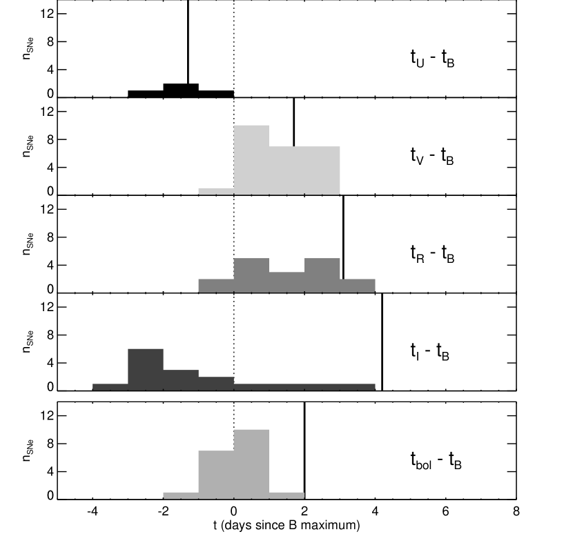
Figure 4: Histograms showing the times of the filter maxima from $\mathit{U}$ to $\mathit{I}$ and of the bolometric luminosity relative to the $\mathit{B}$ maximum. The vertical lines show the time differences as expected for an expanding, adiabatic cooling sphere according to Arnett (arn82 (1982)).

The $\mathit{U}$ band appears to rise faster than the $\mathit{B}$ band, although the limited number of objects (4 supernovae) precludes any definitive statements. The $\mathit{V}$ light curve clearly peaks some time after the $\mathit{B}$ maximum for all observed SNe Ia. This behavior is more or less expected from models of an expanding cooling atmosphere (Arnett arn82 (1982)), as indicated by the lines in Fig. 4. However, the behavior of the $\mathit{R}$ and $\mathit{I}$ band maxima do not agree with this simple model; for these bands, the light curve maxima are reached earlier than in a thermal model. The $\mathit{I}$ histogram is very broad but for most objects the rise in $\mathit{I}$ is clearly faster than in $\mathit{B}$. This trend is further continued in the $\mathit{JHK}$ light curves which all peak before $\mathit{B}$ (Elias et al. eli85 (1985), Leibundgut lei88 (1988), Meikle pme00 (2000)). The early appearance of the peak in the infrared rules out the idea of an expanding, cooling sphere.

5 Bolometric light curves of SNe Ia

The flux emitted by a SN Ia in the UV, optical, and IR wavelengths, the so-called “uvoir bolometric flux”, traces the radiation converted from the radioactive decays of newly synthesized isotopes. As nearly 80% of the bolometric luminosity of a typical SN Ia is emitted in the range from 3000 to 10000 Å (Suntzeff sun96 (1996)), the integrated flux in the $\mathit{UBVRI}$ passbands provides a reliable measure of the bolometric luminosity and therefore represents a physically meaningful quantity. This luminosity depends directly on the amount of nickel produced in the explosion, the energy deposition, and the $\gamma$-ray escape, but not on the exact wavelengths of the emitted photons.

We used the fits of the filter light curves in the $\mathit{UBVRI}$ passbands to construct an optical bolometric light curve for the SNe in our sample. All objects with well-sampled ($\mathit{U}$)$\mathit{BVRI}$ light curves and sufficient coverage from pre-maximum to late decline phases have been included. The objects are listed in Table 1. To calculate the absolute bolometric luminosities, one has to account for reddening and distance moduli; the values we adopted were taken from the literature as listed in Table 1. A galactic extinction law has been employed, as justified by Riess et al. (1996b ).

The bolometric light curves of our sample of SNe Ia are shown in Fig. 5. Only the time range with all available filter photometry is plotted. The peak luminosities are clearly different for the objects in the sample, and these differences are larger than the uncertainties in the derivation. The most striking feature, however, is the varying strength of the secondary shoulder, which stems from the $\mathit{R}$ and $\mathit{I}$ light curves (see also Suntzeff sun96 (1996)).

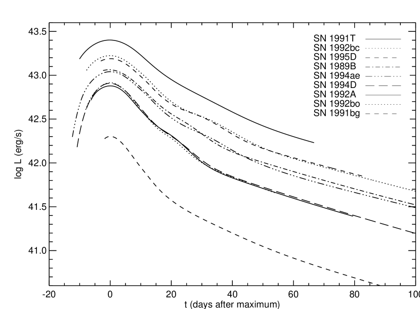
Figure 5: Bolometric luminosities for 9 well observed SNe. Only the time range with the maximum number of filters for each supernova is displayed. The reddening and distance moduli have been taken from the literature as listed in Table 1 and corrections for missing $\mathit{U}$ band are applied as described in Sect. 5.1.1.

The distribution of the epochs of the bolometric peak luminosity relative to the $\mathit{B}$ maximum is shown at the bottom of Fig. 4. The time of bolometric maximum suffers from the additional uncertainty that the contributions from the different wavelength regimes change rapidly before and during the peak phase. Since we are not including any UV flux in our calculations and SNe Ia become optically thin in the UV around this phase, the epoch of the maximum could actually shift to earlier times than what we measure. This might explain the discrepancy with the earlier determination of the bolometric maximum for SN 1990N and SN 1992A by Leibundgut (lei96a (1996)) and Suntzeff (sun96 (1996)), respectively, who included IUE and HST measurements.

5.1 Uncertainties introduced by the data

5.1.1 Missing passbands

Flux outside $\mathit{UBVRI}$:

In our analysis we have neglected any flux outside the optical wavelength range. In particular, contributions to the bolometric flux from the ultraviolet (below 3200 Å) and the infrared above 1 ${\mu}$m ($\mathit{JHK}$) regimes should be considered in the calculations of the bolometric flux. Using HST and IUE spectrophotometry for SN 1990N and SN 1992A, Suntzeff (sun96 (1996)) estimated the fraction of bolometric luminosity emitted in the UV. He found that the bolometric light curve is dominated by the optical flux; the flux in the UV below the optical window drops well below 10% before maximum. The $\mathit{JHK}$ evolution was assumed to be similar to that presented by Elias et al. (eli85 (1985)); these passbands add at most 10% at early times and no more than about 15% 80 days after maximum. For example, examination of the data of SNe 1980N and 1981D (infrared data from Elias et al. (eli81 (1981)) and optical from Hamuy et al. (ham91 (1991))) shows that not more than 6% of the total flux is emitted beyond $\mathit{I}$ until 50 days past maximum, when the IR data stop.

Corrections for passbands missing in the optical range:

For missing passbands between $\mathit{U}$ and $\mathit{I}$ one can infer corrections derived from those SNe Ia which have observations in all filters. Fig. 6 shows the correction factors obtained from SN 1994D. A cautionary note is appropriate here: SN 1994D displayed some unusual features, in particular a very blue color at maximum.

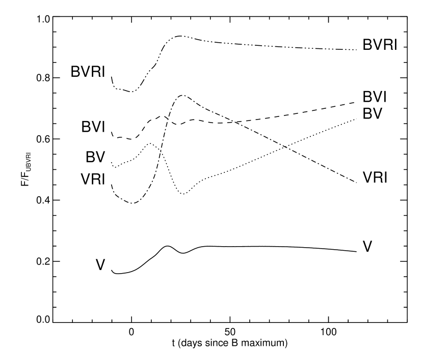
Figure 6: Correction factors for missing passbands. The correction factors are obtained by comparing the flux in the passbands with the total $\mathit{UBVRI}$-flux.

To estimate the flux corrections we divided the flux in each passband by the bolometric flux. Since the filter transmission curves do not continuously cover the spectrum (i. e., there are gaps between $\mathit{U}$ and $\mathit{B}$ as well as between $\mathit{B}$ and $\mathit{V}$ and overlaps between $\mathit{V}$ and $\mathit{R}$, and $\mathit{R}$ and $\mathit{I}$) the coaddition suffers from the interpolation between these passbands.

An interesting result from Fig. 6 is the nearly constant bolometric correction for the $\mathit{V}$ filter. This filter has been used in the past as a surrogate for bolometric light curves (e.g. Cappellaro et al. cap97b (1997)). We confirm the validity of this assumption for phases between 30 and 110 days after $\mathit{B}$ maximum where the overall variation is less than 3%.

In order to test our procedure, we calculated bolometric light curves for the three SNe Ia which have the full wavelength coverage after purposely omitting one or more passbands and applying the correction factors we derived from SN 1994D. As Fig. 7 demonstrates, the error is less than 10% at all times even if more than one filter is missing, although the errors vary considerably during the peak and the secondary shoulder phases. The results of this exercise gave us confidence that we could correct the bolometric light curves of the remaining six SNe for the missing $\mathit{U}$ band without incurring large errors.

Figure 7: Residuals for substituting individual passband observations of SN 1989B by the corrections derived from SN 1994D. The errors never exceed 10% even when more than one filter is missing.

5.1.2 Effects of systematic differences in photometry sets on bolometric light curves

Filter light curves from different observatories often show systematic differences of a few hundredths of a magnitude. We examined the effect such systematic errors might have on our bolometric light curves by artificially shifting individual filter light curves by 0.1 magnitudes and recomputing the bolometric light curves. In all cases the effect on the bolometric light curve is far less than the uncertainties in the distances and the extinction of the supernovae. Shifting the $\mathit{R}$ or $\mathit{I}$ light curve by 0.1 magnitude we found that the bolometric luminosity changed by 2% at maximum and 5% 25 days later (approximately at second maximum). For typical systematic uncertainties of 0.03 magnitudes in all filters, a maximal error of 2 to 3% is incurred.

We also constructed the bolometric light curve of SN 1994D for the individual data sets available (see references to Table 1). The difference never exceeds 4% out to 70 days after maximum even though the photometry in the individual filters differs up to 0.2 magnitudes in $\mathit{U}$, 0.1 mag in $\mathit{BRI}$ and 0.05 mag in $\mathit{V}$.

5.2 Uncertainties introduced by external parameters

While uncertainties in the distance moduli will affect the absolute luminosities in each passband (as well as the bolometric luminosity), the shape of the light curve is unaffected. As all distances used here are scaled to a Hubble constant of $H_{0}=65\,\mathrm{km\,s^{-1}\,Mpc^{-1}}$, the luminosity differences are affected only by errors in the determination of the relative distance modulus.

Reddening, however, affects both the absolute luminosity and the light curve shape. The influence of extinction changes as a function of phase with the changing color of the supernova. A color excess of $\mathit{E(B-V)}$ $=0.05$ decreases the observed bolometric luminosity at $t=t_{\mathrm{max}}(\mathrm{bol})$ by 15%, while near the time of the second maximum in the $\mathit{R}$ and $\mathit{I}$ light curves ($t=20\,\mathrm{days}$) the observed bolometric luminosity is reduced by 12%. A stronger extinction of $\mathit{E(B-V)}$ $=0.35$ reduces the observed bolometric luminosity by 67% (56%) at $t=t_{\mathrm{max}}$ ($t=20\,\mathrm{days}$).

The uncertainty in the reddening estimate introduces subtle additional effects. If $\delta$$\mathit{E(B-V)}$$=0.02$ mag at low reddenings ($\mathit{E(B-V)}$$<0.05$), an additional uncertainty of 5% in the bolometric luminosity is introduced. At higher reddening values ($\mathit{E(B-V)}$ $=0.3$), uncertainties of $\delta$$\mathit{E(B-V)}$=0.05 and 0.10 produce changes of 15% and 31% in the bolometric luminosity, respectively.

The decline rate of the bolometric light curve decreases with increasing reddening due to the color evolution of the supernova and the selective absorption. For SN 1994D $\Delta m_{15}$(Bol) would evolve linearly from 1.13 at hypothetical $\mathit{E(B-V)}$ $=0$ to 0.99 at $\mathit{E(B-V)}$ $=0.35$. The linearity breaks down at about $\mathit{E(B-V)}$ $\approx 0.5$.

As described by Leibundgut (lei88 (1988)) the reddening depends on the intrinsic color of the observed object (Schmidt-Kaler sch82 (1982)). This implies that the color evolution influences the shape of the filter light curves. A color difference of $\mathit{B-V}$$=0.7$ for SNe Ia in the first 15 days results in an increase of $\Delta m_{15}$($\mathit{B}$) by $0.2\times{\mbox{$\mathit{E(B-V)}$}}$ simply due to the color dependence of the reddening. The increase of $\Delta m_{15}$ for blue filters is larger than for the redder passbands.

5.3 Uncertainties introduced by the method

The effect of fitting the light curves before constructing the bolometric light curves can be seen in Fig. 8. The bolometric flux for SN 1992bc determined in this way is compared against the straight integration over the wavelengths of the filter observations. The agreement between the two approaches is excellent and no differences can be observed. This also applies to the correction for the missing $\mathit{U}$ filter observations. Deviations can be found only for those parameters derived from the light curve, which extrapolate far from the observed epochs, e.g. the rise time.

Figure 8: Constructing the bolometric light curves before and after fitting the filter light curves of SN 1992bc. The stars indicate the bolometric luminosity as calculated directly from the observations. The correction for missing $\mathit{U}$ band is applied as described in Sect. 5.1.1, only the epochs with the maximum number of filters are shown. The dotted line is the bolometric luminosity calculated from the fits to the individual passbands.

The integration over wavelengths to calculate the bolometric light curve can be performed in different ways. A straight integration of the broad-band fluxes has to take into account the transmission of and any overlaps and gaps between filters. We experimented with several integration techniques, but found that for all interpolation methods, we reproduced the bolometric flux to within 2% at any epoch we considered. This has already been shown for SN 1987A by Suntzeff & Bouchet (sun90 (1990)). We chose to calculate the bolometric flux by summing the flux at the effective filter wavelength multiplied with the filter bandwidth.

6 Discussion

6.1 Peak Bolometric Flux

The bolometric light curves presented in Fig. 5 were constructed from $\mathit{UBVRI}$ light curves where available (SN 1989B, SN 1991T and SN 1994D). All others are based on $\mathit{BVRI}$ light curves with a correction for the missing $\mathit{U}$ band applied as described in Sect. 5.1.1. The luminosities depend directly on the assumed distance moduli to the individual supernovae. We have used the current best estimates from the literature (Table 1), but some of the distance estimates may change when more accurate distances become available. We also corrected the magnitudes for extinction, which, for some objects, can be fairly substantial (SN 1989B, SN 1991T, and SN 1994ae). From Table 2 it is clear that our sample displays a rather large range in luminosities, both in $\mathit{B}$ and the bolometric maximum. SN 1991bg is 11 times less luminous in $\mathit{B}$ than the brightest SN Ia in the sample, SN 1991T. For the bolometric maximum we find a factor of 12.3. Excluding this peculiar object we still find a range in luminosity of a factor 4.7 in the filter passband and a factor of 3.3 in the bolometric peak flux.

6.2 Light Curve Shape

The shapes of the bolometric light curves are unaffected by the distance modulus and are only marginally influenced by reddening (see Sect. 5). The most striking feature in these light curves is the inflection near 25 days past maximum (Suntzeff sun96 (1996)). It is observed in all SNe Ia, with the notable exception of SN 1991bg (Fig. 5). The strength of this shoulder varies from a rather weak flattening in the bolometric light curve of SN 1991T to a very strong bump in SN 1994D. This bump arises from the strong secondary maximum in the $\mathit{R}$ and $\mathit{I}$ light curves. The secondary maximum is also observed in the near-IR $\mathit{JHK}$ light curves (Elias et al. eli85 (1985), Meikle pme00 (2000), Meikle & Hernandez mei00 (2000)) which have not been used for the calculation of bolometric light curves presented here.

Table 2: Absolute $\mathit{B}$ magnitudes and bolometric luminosities. The bolometric luminosities have been corrected for the missing $\mathit{U}$ band where appropriate. The nickel mass is derived from the luminosity for a rise time of 17 days to the bolometric peak.

SN	$M_{\mbox{$\mathit{B}$}}$	$\Delta m_{15}^{\mbox{$\mathit{B}$}}$	$\log L_{\mathrm{bol}}$	$\Delta m_{15}^{\mathrm{bol}}$	$M_{\mathrm{Ni}}$	$t_{-1/2}$	$t_{+1/2}$
	(mag)	(mag)	(erg s-1)	(mag)	($M_{\sun}$)	(days)	(days)
(1)	(2)	(3)	(4)	(5)	(6)	(7)	(8)
SN1989B	-19.37	1.20	43.06	0.91	0.57	—	13.1
SN1991T	-20.06	0.97	43.36	0.83	1.14	11.6	14.0
SN1991bg	-16.78	1.85	42.32	1.42	0.11	—	8.8
SN1992A	-18.80	1.33	42.88	1.15	0.39	8.6	10.3
SN1992bc	-19.72	0.87	43.22	0.93	0.84	10.1	13.0
SN1992bo	-18.89	1.73	42.91	1.27	0.41	8.3	9.6
SN1994D	-18.91	1.46	42.91	1.16	0.41	7.5	10.8
SN1994ae	-19.24	0.95	43.04	0.97	0.55	9.6	12.6
SN1995D	-19.66	0.98	43.19	1.00	0.77	—	12.2

Inspection of Fig. 5 clearly shows the brighter SNe having wider primary peaks than the fainter SNe.

In order to quantify this statement we have measured the width of the bolometric light curve at half the peak luminosity (with $t_{-1/2}$ denoting the time it takes to rise and $t_{+1/2}$ to decline, see Table 2). There are sufficient pre-maximum observations available for six supernovae (SN 1991T, SN 1992A, SN 1992bc, SN 1992bo, SN 1994D, and SN 1994ae) from which the full width of the peaks can be reliably determined. In three cases the first observations were obtained well below the half-maximum flux level; in the case of SN 1991T we extrapolated our bolometric light curve by about 1.5 days and for SN 1992A and SN 1992bc by 2.5 days. The bright SN 1991T and SN 1992bc show a peak width of 26 and 23 days, respectively, the intermediate SN 1994ae one of 22 days, while the fainter SN 1994D, SN 1992A, and SN 1992bo remained brighter than half their maximum luminosity for about 18 to 19 days.

The pre-maximum rise $t_{-1/2}$ in the bolometric light curve is, in all cases, substantially faster than the decline $t_{+1/2}$ by between 20 to 30% or a time difference of between 2 to almost 4 days (Table 2).

The decline to half the supernova’s peak luminosity $t_{+1/2}$ varies from 9 days to 14 days. A weak correlation between maximum brightness and decline rate can be seen (Fig. 9). The sample of SNe was extended to the one used in Sect. 4. In Fig. 9 only those SNe with sufficient time coverage are shown.

Figure 9: Rise to and decline from maximum in bolometric light curves. The time between maximum luminosity and half its value is plotted. The sample of SNe was extended to the one used in Sect. 4, the SNe from Table 1 are shown as filled symbols. Only SNe with sufficient coverage (rise: first observation not later than 3 days after $t_{-1/2}$, decline: first observation before $t_{\mathrm{max}}$(Bol)) have been included.

Significant coverage of the rise to maximum is available for only two supernovae. There are too few SNe to make a definitive statement here about the rise times of SNe Ia in general. Nevertheless, our formal fits to SN 1994D and SN 1994ae give rise times of 16.4 and 18.2 days, respectively, for their bolometric light curves. The formal errors in this parameter, derived with the Monte Carlo algorithm described in Sect. 3.2, is 2 days for SN 1994D and 1 day for SN 1994ae. If the bolometric luminosities are calculated by fitting the bolometric light curve from the individual observations, the derived rise times are slightly different ($18$ and $19$ days, respectively). A previous analysis of SN 1994D derived a rise time for the bolometric light curve of 18 days (Vacca & Leibundgut vac96 (1996)) in fair agreement with our current analysis.

These rise times are significantly larger than most light curve calculation of explosion models (Höflich et al. hoe96 (1996), Pinto & Eastman 2000a ). These theoretical calculations typically yield rise times of 15 days.

The secondary bump clearly indicates a change in the emission mechanism of SNe Ia. Its varying strength might be related to the release of photons “stored” in the ejecta (the “old” photons described in Pinto & Eastman 2000b and Eastman eas97 (1997)). In such a scenario the bump arises from the fact that the ejecta become optically thin during this phase, due to subtle differences in the ejecta structure and ejecta velocity.

The exponential decline of the bolometric light curves between 50 and 80 days past bolometric maximum is remarkably similar for all supernovae. The decline at this phase is still dominated by the $\@element[56]{\mathrm{Co}}$ decay and the $\gamma-$ray escape fraction (Milne et al. mil99 (1999)). We find a decline rate of 2.6$\pm$0.2 mag per 100 days. The sample is still very small but SN 1991bg stands out with a decline rate of 3.0 mag/(100 days). The uniformity of the late declines indicates that the differences observed at earlier phases are due to photospheric effects when the optical depth for optical radiation is large and not because of the explosion mechanism. In particular the fraction of energy converted to optical radiation at late phases appears to change in an identical fashion for the majority of the objects, although SN 1991bg proves to be the exception to the rule once again. The change in the column density in the different supernovae must be very similar, despite the different luminosities at these epochs. This indicates that the kinetic energy is somehow coupled to the pre-supernova mass.

The decline rate during the same period in the $\mathit{V}$ filter is identical with 2.6$\pm$0.2 mag/(100 days) as is also confirmed by the constant fraction of the $\mathit{V}$ to the bolometric flux (cf. Fig. 6). These decline rates have been shown to correlate very well with measurements derived by others (Vacca & Leibundgut vac97 (1997)). The comparison with other determinations of the decline rate is difficult as the slope of the decline continues to vary even at late epochs (e.g. Suntzeff sun96 (1996), Turatto et al. tur96a (1996)). This dependence on the epochs observed has to be considered when a comparison is attempted. In most cases the decline was estimated out to phases of 200 days (Turatto et al. tur90 (1990)), which leads to smaller decline rates than we find here. In the case of SN 1991bg the decline rate was measured at early phases, which led to a significantly steeper decline estimate (Filippenko et al. fil92a (1992)).

Note that the phase range of bolometric light curves presented in this paper is well before any effects of positron escape could be measured (Milne et al. mil99 (1999)) or the IR catastrophe takes place (Fransson et al. fra96 (1996)).

6.3 Nickel mass

Given the peak luminosity it is straight forward to derive the nickel mass which powers the supernova emission. Near maximum light the photon escape equals the instantaneous energy input and is directly related to the total amount of $\@element[56]{\mathrm{Ni}}$ synthesized in the explosion (Arnett arn82 (1982), Arnett et al. arn85 (1985), Pinto & Eastman 2000a ). We have used our bolometric peak luminosities to derive the nickel masses (Table 2). Since we are not sampling all the emerging energy from the SNe Ia, but are restricted to the optical fluxes, we are underestimating the total luminosity. Suntzeff (sun96 (1996)) estimated that about 10% are not accounted by the optical filters near maximum light. All masses thus have to be increased by a factor 1.1. Another uncertainty is the exact rise time, which is an important parameter in the calculation. We have assumed a rise time of 17 days to the bolometric maximum for all supernovae. It is likely that there are significant differences in the rise times and this would alter the estimates for the Ni mass. A longer rise time would imply a larger nickel mass for a given measured luminosity. Decreasing the rise time to 12 days yields only 70% $M_{\mathrm{Ni}}$ of the values given in Table 2. Such a short rise time is excluded for most of the SNe Ia, where observations as early as 14 days have been recorded (SN 1990N: Leibundgut et al. 1991a , Lira et al. lir98 (1998), SN 1994D: Vacca & Leibundgut vac96 (1996)), but could still be feasible for SN 1991bg. For a more realistic range of 16 to 20 days between explosion and bolometric maximum the nickel mass would change by only $\mp$10% from the values provided here. Clearly, the dominant uncertainty in the determination of the nickel mass stems from the uncertainties in the distances and the extinction corrections.

For a few of the supernovae, nickel masses have been measured by other methods. SN 1991T has an upper limit for the radioactive nickel produced in the explosion of about 1 $M_{\sun}$ based on the 1.644$\mu$m Fe lines (Spyromilio et al. spy92 (1992)). This value depends on the exact ionization structure of the supernova one year after explosion and a conservative range of 0.4 to 1 $M_{\sun}$ had been derived. This is fully consistent with our estimate. Bowers et al. (bow97 (1997)) have derived nickel masses for several SNe Ia in a similar way. Their best estimates for SN 1991T, SN 1994ae, and SN 1995D are all about half the value found here, when converted to their distances and extinctions. However, they point out that their values should be increased by a factor of 1.2 to 1.7 to account for ionization states not included in their analysis. With this correction we find a good agreement. Cappellaro et al. (cap97b (1997)) derived masses from the late $\mathit{V}$ light curves. There are four objects in common with our study: SN 1991bg, SN 1991T, SN 1992A, and SN 1994D. Adjusting the determinations to the same distances and re-normalizing to our SN 1991T Ni mass, we find a general agreement, although there are differences at the 0.1 $M_{\sun}$ level.

Nickel masses were also derived from the line profiles of [Fe II] and [Fe III] lines in the optical by Mazzali et al. (ma98 (1998)). These measurements depend critically on the ionization structure in the ejecta and had been normalized to a nickel mass of SN 1991T of 1 $M_{\sun}$. When we scale their masses to our measurement we find a reasonable agreement.

The nickel masses derived in our analysis are well within the bounds of the current models for SN Ia explosions (Höflich et al. hoe96 (1996), Woosley & Weaver woo94 (1994)). There seems to be no real difference in $\@element[56]{\mathrm{Ni}}$ produced by the various explosion models and hence a distinction by the bolometric light curve alone is not possible.

7 Conclusions

Fitting light curves with a descriptive model has a number of advantages over template methods. It is suited to explore the variety among SN Ia and provides an independent way to look for correlations. A simple application of our fitting procedure has been presented to demonstrate the complicated nature of SN Ia emission through the occurrence of the peak luminosity in individual filters. The most obvious signatures for non-thermal emission from SNe Ia have so far been the infrared light curves (Elias et al. eli85 (1985)) and the lack of emission near 1.2$\mu$m (Spyromilio et al. spy94 (1994), Wheeler et al. whe98 (1998)). It had also been demonstrated through spectral synthesis calculations (Höflich et al. hoe96 (1996), Eastman eas97 (1997)). Although there is a fairly large scatter of about 2 days in the relative epoch of filter maximum light a clear trend to earlier maxima in $\mathit{R}$ and $\mathit{I}$ is observed. In fact, the $\mathit{I}$ maximum occurs clearly before the $\mathit{B}$ maximum, a trend also observed in the $\mathit{JHK}$ light curves (Elias et al. eli85 (1985), Meikle pme00 (2000)).

Another application of the continuous approximation of the observations is the construction of bolometric light curves. Bolometric light curves form an important link between the explosion models and the radiation transport calculations for SNe Ia ejecta. We have demonstrated that the effects of missing passbands, distance modulus, reddening, light curve fitting and the integration methods are not critical to the shape. Amongst these, the uncertainties from the distance modulus towards individual supernovae dominate.

The shapes of the bolometric light curve of individual SNe Ia vary significantly. The secondary maxima observed in the $\mathit{R}$ and $\mathit{I}$ light curves show up with varying strength in the bolometric light curves as well. The variety of light curve shapes indicates subtle variations in the energy release of these explosions. Pinto & Eastman (2000b ) try to explain these secondary maxima as due to the distribution of material in the inner core of the explosion, possibly connected to the explosion mechanism. If this is the case, then the detailed study of the bolometric light curves and their differences among individual SNe Ia might provide a direct “window” into the explosion.

With the currently best available distances we find that the peak luminosities of the SNe Ia in our sample display a rather large range. They imply a factor of 2.5 in the $\@element[56]{\mathrm{Ni}}$ masses. SN 1991bg produced about 8 times less $\@element[56]{\mathrm{Ni}}$ than the brightest object, SN 1992bc. The range of nickel masses indicates significant differences in the explosions of SNe Ia. From the late-phase decline, we find that the change of the decline rate is rather uniform indicating similarity in change of the $\gamma-$ray escape fraction for all SNe Ia independent of the amount of nickel produced in the explosion.

- (1) Arnett W. D., 1982, ApJ 253, 785
- (2) Arnett W. D., Branch D., Wheeler J. C., 1985, Nat 314, 337
- (3) Bowers E. J. C., Meikle W. P. S., Geballe T. R., et al., 1997, MNRAS 290, 663
- (4) Branch D., Tammann G. A., 1992, ARA&A 30, 359
- (5) Cappellaro E., Mazzali P. A., Benetti S., et al., 1997, A&A 328, 203
- (6) Doggett J. B., Branch D., 1985, AJ 90, 2303
- (7) Eastman R. G., 1997, In: Thermonuclear Supernovae, Ruiz-Lapuente P., Canal R., Isern J. (eds.), Kluwer, Dordrecht, p. 571
- (8) Elias J. H., Frogel J. A., Hackwell J. A., et al., 1981, ApJ 251, L13
- (9) Elias J. H., Matthews K., Neugebauer G., et al., 1985, ApJ 296, 379
- (10) Filippenko A. V., Richmond M. W., Branch D., et al., 1992, AJ 104, 1543
- (11) Fisher A., Branch D., Hatano K., et al., 1999, MNRAS 304, 67
- (12) Fransson C., Houck J., Kozma C., 1996, In: IAU Colloquium 145: Supernovae and Supernova Remnants, McCray R., Wang Z. (eds.), Cambridge University Press, Cambridge, p. 211
- (13) Frogel J. A., Gregory B., Kawara K., et al., 1987, ApJ 315, L129
- (14) Garnavich P. M., Kirshner R. P., Challis P., et al., 1998, ApJ 493, L53
- (15) Hamuy M., Phillips M. M., Maza J., et al., 1991, AJ 102, 208
- (16) Hamuy M., Phillips M. M., Schommer R. A., et al., 1996a, AJ 112, 2391
- (17) Hamuy M., Phillips M. M., Suntzeff N. B., et al., 1996b, AJ 112, 2408
- (18) Höflich P., Khokhlov A., Wheeler J. C., et al., 1996, ApJ 472, L81
- (19) Höflich P., Khokhlov A., Wheeler J., et al., 1997, In: Thermonuclear Supernovae, Ruiz-Lapuente P., Canal R., Isern J. (eds.), Kluwer, Dordrecht, p. 659
- (20) Khokhlov A., Müller E., Höflich P., 1993, A&A 270, 223
- (21) Leibundgut B., 1988, Ph.D. thesis, Universität Basel
- (22) Leibundgut B., 1996, In: IAU Colloquium 145: Supernovae and Supernova Remnants, McCray R., Wang Z. (eds.), Cambridge University Press, Cambridge, p. 11
- (23) Leibundgut B., Pinto P. A., 1992, ApJ 401, 49
- (24) Leibundgut B., Kirshner R. P., Filippenko A. V., et al., 1991a, ApJ 371, L23
- (25) Leibundgut B., Tammann G. A., Cadonau R., et al., 1991b, A&AS 89, 537
- (26) Leibundgut B., Kirshner R. P., Phillips M. M., et al., 1993, AJ 105, 301
- (27) Lira P., Suntzeff N. B., Phillips M. M., et al., 1998, AJ 115, 234
- (28) Mazzali P. A., Cappellaro E., Danziger I. J., et al., 1998, ApJ 499, L49
- (29) Meikle W. P. S., 2000, MNRAS 314, 782
- (30) Meikle W. P. S., Hernandez M., 2000, In: Future Directions of Supernova Research, Cassisi S. Mazzali P. (eds.), Mem. Soc. Astron. Ital., in press (astro-ph/9902056)
- (31) Meikle W. P. S., Cumming R. J., Geballe T. R., et al., 1996, MNRAS 281, 263
- (32) Milne P. A., The L.-S., Leising M., 1999, ApJS 124, 503
- (33) Minkowski R., 1964, ARA&A 2, 247
- (34) Patat F., Benetti S., Cappellaro E., et al., 1996, MNRAS 278, 111
- (35) Perlmutter S., Gabi S., Goldhaber G., et al., 1997, ApJ 483, 565
- (36) Phillips M. M., 1993, ApJ 413, L105
- (37) Phillips M. M., Phillips A. C., Heathcote S. R., et al., 1987, PASP 99, 592
- (38) Phillips M. M., Lira P., Suntzeff N. B., et al., 1999, AJ 118, 1766
- (39) Pinto P. A., Eastman R. G., 2000a, ApJ 530, 744
- (40) Pinto P. A., Eastman R. G., 2000b, ApJ 530, 757
- (41) Richmond M. W., Treffers R. R., Filippenko A. V., et al., 1995, AJ 109, 2121
- (42) Riess A. G., 1996, Ph.D. thesis, Harvard University, Cambridge, MA
- (43) Riess A. G., Press W. H., Kirshner R. P., 1996a, ApJ 473, 88
- (44) Riess A. G., Press W. H., Kirshner R. P., 1996b, ApJ 473, 588
- (45) Riess A. G., Filippenko A. V., Challis P., et al., 1998a, AJ 116, 1009
- (46) Riess A. G., Nugent P., Filippenko A. V., et al., 1998b, ApJ 504, 935
- (47) Riess A. G., Kirshner R. P., Schmidt B. P., et al., 1999, AJ 117, 707
- (48) Sadakane K., Yokoo T., Arimoto J.-I., et al., 1996, PASJ 48, 51
- (49) Saha A., Sandage A., Tammann G. A., et al., 1999, ApJ 522, 802
- (50) Schlegel E. M., 1995, AJ 109, 2620
- (51) Schlegel D. J., Finkbeiner D. P., Davis M., 1998, ApJ 500, 525
- (52) Schmidt-Kaler T., 1982, In: Landolt-Börnstein Vol. VI/2b, Schaifer K., Voigt H. (eds.), Springer, Berlin, p. 10
- (53) Schmidt B. P., Suntzeff N. B., Phillips M. M., et al., 1998, ApJ 507, 46
- (54) Spyromilio J., Meikle W. S. P., Allen D. A., et al., 1992, MNRAS 258, 53
- (55) Spyromilio J., Pinto P. A., Eastman R. G., 1994, MNRAS 266, L17
- (56) Suntzeff N. B., 1996, In: IAU Colloquium 145: Supernovae and Supernova Remnants, McCray R., Wang Z. (eds.), Cambridge University Press, Cambridge, p. 41
- (57) Suntzeff N. B., Bouchet P., 1990, AJ 99, 650
- (58) Suntzeff N. B., Phillips M. M., Covarrubias R., et al., 1999, AJ 117, 1175
- (59) Turatto M., Cappellaro E., Barbon R., et al., 1990, AJ 100, 771
- (60) Turatto M., Benetti S., Cappellaro E., et al., 1996, MNRAS 283, 1
- (61) Vacca W. D., Leibundgut B., 1996, ApJ 471, L37
- (62) Vacca W. D., Leibundgut B., 1997, In: Thermonuclear Supernovae, Ruiz-Lapuente P., Canal R., Isern J. (eds.), Kluwer, Dordrecht, p. 65
- (63) Wells L. A., Phillips M. M., Suntzeff N. B., et al., 1994, AJ 108, 2233
- (64) Wheeler J. C., Höflich P., Harkness R. P., et al., 1998, ApJ 496, 908
- (65) Woosley S. E., Weaver T. A., 1994, ApJ 423, 371