Numerical Simulations in Cosmology III: Dark Matter Halos

Abstract

We give a review of different properties of dark matter halos. Taken from different publications, we present results on (1) the mass and velocity functions, (2) density and velocity profiles, and (3) concentration of halos. The results are not sensitive to parameters of cosmological models, but formally most of them were derived for popular flat $\Lambda$CDM  model. In the range of radii $r=(0.005-1)\mbox{$r_{\rm vir}$}$ the density profile for a quiet isolated halo is very accurately approximated by a fit suggested by Moore et al.(1997): $\rho\propto 1/x^{1.5}(1+x^{1.5})$, where $x=r/\mbox{$r_{\rm s}$}$ and $r_{\rm s}$  is a characteristic radius. The fit suggested by Navarro et al.(1995) $\rho\propto 1/x(1+x)^{2}$, also gives a very satisfactory approximation with relative errors of about 10% for radii not smaller than 1% of the virial radius. The mass function of $z=0$ halos with mass below $\approx 10^{13}\mbox{$h^{-1}$M${}_{\odot}$}$ is approximated by a power law with slope $\alpha=-1.85$. The slope increases with the redshift. The velocity function of halos with $\mbox{$V_{\rm max}$}<500$ km/s is also a power law with the slope $\beta=-3.8-4$. The power-law extends to halos at least down to 10 km/s. It is also valid for halos inside larger virialized halos. The concentration of halos depends on mass (more massive halos are less concentrated) and environment, with isolated halos being less concentrated than halos of the same mass inside clusters. Halos have intrinsic scatter of concentration: at $1\sigma$ level halos with the same mass have $\Delta(\log{c_{\rm vir}})=0.18$ or, equivalently, $\Delta\mbox{$V_{\rm max}$}/\mbox{$V_{\rm max}$}=0.12$. Velocity anisotropyfor both subhalos and the dark matter is approximated by $\beta(r)=0.15+2x/[x^{2}+4]$, where $x$ is radius in units of the virial radius.

1 Introduction

During the last decade there was an increasingly growing interest in testing predictions of variants of the cold dark matter (CDM) models at subgalactic ($\lesssim 100{\rm\ kpc}$) scales. This interest was first induced by indications that observed rotation curves in the central regions of dark matter dominated dwarf galaxies are at odds with predictions of hierarchical models. Specifically, it was argued (Moore 1994; Flores & Primack 1994) that circular velocities, $v_{c}(r)\equiv[GM(<r)/r]^{1/2}$, at small galactocentric radii predicted by the models are too high and increase too rapidly with increasing radius compared to the observed rotation curves. The steeper than expected rise of $v_{c}(r)$ implies that the shape of the predicted halo density distribution is incorrect and/or that the DM halos formed in CDM models are too concentrated (i.e., have too much of their mass concentrated in the inner regions).

In addition to the density profiles, there is an alarming mismatch in predicted abundance of small-mass ($\lesssim 10^{8}-10^{9}\mbox{$h^{-1}$M${}_{\odot}$}$) galactic satellites and the observed number of satellites in the Local Group (Kauffmann, White & Guiderdoni 1993; Klypin et al. 1999; Moore et al. 1999). Although this discrepancy may well be due to feedback processes such as photoionization that prevent gas collapse and star formation in the majority of the small-mass satellites (e.g., Bullock, Kravtsov & Weinberg 2000), the mass scale at which the problem sets in is similar to the scale in the spectrum of primordial fluctuations that may be responsible for the problems with density profiles. In the age of precision cosmology that forthcoming MAP and Planck cosmic microwave background anisotropy satellite missions are expected to bring, tests of the cosmological models at small scales may prove to be the final frontier and the ultimate challenge to our understanding of the cosmology and structure formation in the Universe. However, this obviously requires detailed predictions and checks from the theoretical side and higher resolution/quality observations and thorough understanding of their implications and associated caveats from the observational side. In this paper we focus on the theoretical predictions of the density distribution of DM halos and some problems with comparing these predictions to observations.

A systematic study of halo density profiles for a wide range of halo masses and cosmologies was done by Navarro, Frenk & White (1996, 1997; hereafter NFW), who argued that analytical profile of the form $\rho(r)=\rho_{s}(r/r_{s})^{-1}(1+r/r_{s})^{-2}$ provides a good description of halo profiles in their simulations for all halo masses and in all cosmologies. Here, $r_{s}$ is the scale radius which, for this profile corresponds to the scale at which $d\log\rho(r)/d\log r|_{r=r_{s}}=-2$. The parameters of the profile are determined by the halo’s virial mass $M_{\rm vir}$ and concentration defined as $c\equiv\mbox{$r_{\rm vir}$}/r_{s}$. NFW argued that there is a tight correlation between $c$ and $M_{\rm vir}$, which implies that the density distributions of halos of different masses can in fact be described by a one-parameter family of analytical profiles. Further studies by Kravtsov, Klypin & Khokhlov (1997), Kravtsov et al. (1999), Jing (1999), Bullock et al. (2000), although confirming the $c(\mbox{$M_{\rm vir}$})$ correlation, indicated that there is a significant scatter in the density profiles and concentrations for DM halos of a given mass.

Following the initial studies by Moore (1994) and Flores & Primack (1994), Kravtsov et al. (1999) presented a systematic comparison of the results of numerical simulations with rotation curves of a sample of seventeen dark matter dominated dwarf and low surface brightness (LSB) galaxies. Based on these comparisons, we argued that there does not seem to be a significant discrepancy in the shape of the density profiles at the scales probed by the numerical simulations ($\gtrsim 0.02-0.03\mbox{$r_{\rm vir}$}$, where $r_{\rm vir}$ is halo’s virial radius). However, these conclusions were subject to several caveats and had to be tested. First, observed galactic rotation curves had to be re-examined more carefully and with higher resolution. The fact that all of the observed rotation curves used in earlier analyses were obtained using relatively low-resolution HI observations, required checks of the possible beam smearing effects. Also, a possibility of non-circular random motions in the central regions that could modify the rotation velocity of the gas (e.g., Binney & Tremain 1987, p. 198) had to be considered. Second, the theoretical predictions had to be tested for convergence and extended to scales $\lesssim 0.01\mbox{$r_{\rm vir}$}$.

Moore et al. (1998; see also a more recent convergence study by Ghigna et al. 1999) presented a convergence study and argued that mass resolution has a significant impact on the central density distribution of halos. They argued that at least several million particles per halo are required to model reliably the density profiles at scales $\lesssim 0.01\mbox{$r_{\rm vir}$}$. Based on these results, Moore et al. (1999) advocated a density profile of the form $\rho(r)\propto(r/r_{0})^{-1.5}[1+(r/r_{0})^{1.5}]^{-1}$, that behaves similarly ($\rho\propto r^{-3}$) to the NFW profile at large radii, but is steeper at small $r$: $\rho\propto r^{-1.5}$. Most recently, Jing & Suto (2000) presented a systematic study of density profiles for halo masses range $2\times 10^{12}\mbox{$h^{-1}$M${}_{\odot}$}-5\times 10^{14}\mbox{$h^{-1}$M${}_{\odot}$}$. The study was uniform in mass and force resolution featuring $\sim 5-10\times 10^{5}$ particles per halo and force resolution of $\approx 0.004\mbox{$r_{\rm vir}$}$. They found that galaxy-mass halos in their simulations are well fitted by profile $\rho(r)\propto(r/r_{0})^{-1.5}[1+r/r_{0}]^{-1.5}$, but that cluster-mass halos are well described by the NFW profile, with logarithmic slope of the density profiles at $r=0.01\mbox{$r_{\rm vir}$}$ changing from $\approx-1.5$ for $\mbox{$M_{\rm vir}$}\sim 10^{12}\mbox{$h^{-1}$M${}_{\odot}$}$ to $\approx-1.1$ for $\mbox{$M_{\rm vir}$}\sim 5\times 10^{14}\mbox{$h^{-1}$M${}_{\odot}$}$. Jing & Suto interpreted these results as evidence that profiles of DM halos are not universal.

Rotation curves of a number of dwarf and LSB galaxies have recently been reconsidered using H$\alpha$ observations (e.g., Swaters, Madore & Trewhella 2000; van den Bosch et al. 2000). The results show that for majority of galaxies H$\alpha$ rotation curves are significantly different in their central regions than the rotation curves derived from HI observations. This indicates that the HI rotation curves are affected by beam smearing (Swaters et al. 2000). It is also possible that some of the difference may be due to real differences in kinematics of the two tracer gas components (ionized and neutral hydrogen). Preliminary comparisons of the new H$\alpha$ rotation curves with model predictions show that NFW density profiles are consistent with the observed shapes of rotation curves (van den Bosch 2000; Navarro & Swaters 2000). Moreover, cuspy density profiles with inner logarithmic slopes as steep as $\sim-1.5$ also seem to be consistent with the data (van den Bosch 2000). Nevertheless, CDM halos appear to be too concentrated (Navarro & Swaters 2000; McGaugh et al. 2000; Navarro & Steinmetz 2000) as compared to galactic halos, and therefore the problem remains.

New observational and theoretical developments show that comparison of model predictions to the data is not straightforward. Decisive comparisons require reaching convergence of theoretical predictions and understanding the kinematics of the gas in the central regions observed galaxies. In this paper we present convergence tests designed to test effects of mass resolution on the density profiles of halos formed in the currently popular CDM model with cosmological constant ($\Lambda$CDM) and simulated using the multiple mass resolution version of the Adaptive Refinement Tree code (ART). We also discuss some caveats in drawing conclusions about the density profiles from the fits of analytical functions to numerical results and their comparisons to the data.

2 Dark Matter Halos: the NFW and the Moore et al. profiles

Before we fit the analytical profiles to real dark matter halos or compare them with observed rotational curves, it is instructive to compare different analytical approximations. Although the NFW and Moore et al. profiles predict different behavior of $\rho(r)$ in the central regions of a halo, the scale where this difference becomes significant depends on the specific values of halo’s characteristic density and radius. Table 2 presents different parameters and statistics associated with the two analytical profiles. For the NFW profile more information can be found in Klypin et al. (1999), Lokas & Mamon (2000), and in Widrow (2000).

Each profile is set by two independent parameters. We choose these to be the characteristic density $\rho_{0}$ and radius $r_{s}$. In this case all expressions describing different properties of the profiles have simple form and do not depend on concentration. The concentration or the virial mass appear only in the normalization of the expressions. The choice of the virial radius (e.g., Lokas & Mamon 2000) as a scale unit results in more complicated expressions with explicit dependence on the concentration. In this case, one also has to be careful about definition of the virial radius, as there are several different definitions in the literature. For example, it is often defined as the radius, $r_{200}$, within which the average density is 200 times the critical density. In this paper the virial radius is defined as radius within which the average density is equal to the density predicted by the top-hat model: it is $\delta_{\rm TH}$ times the average matter density in the Universe. For the $\Omega_{0}=1$ case the two existing definitions are equivalent. In the case of $\Omega_{0}=0.3$ models, however, the virial radius is about 30% larger than $r_{200}$.

There is no unique way of defining a consistent concentration for the different analytical profiles. Again, it is natural to use the characteristic radius $r_{s}$ to define the concentration: $c\equiv r_{\rm vir}/r_{s}$. This simplifies expressions. At the same time, if we fit the same dark matter halo with the two profiles, we will get different concentrations because the values of corresponding $r_{s}$ will be different. Alternatively, if we choose to match the outer parts of the profiles (say, $r>r_{s}$) as closely as possible, we may choose to change the ratio of the characteristic radii $r_{s,\rm NFW}/r_{s,\rm Moore}$ in such a way that both profiles reach the maximum circular velocity $v_{\rm circ}$ at the same physical radius $r_{\rm max}$. In this case, the formal concentration of the Moore et al. profile is 1.72 times smaller than that of the NFW profile. Indeed, with this normalization profiles look very similar in the outer parts as one finds in Figure 1. Table 2 also gives two other “concentrations”. The concentration $C_{1/5}$ is defined as the ratio of virial radius to the radius, which encompasses 1/5 of the virial mass (Avila-Reese et al. 1999). For halos with $C_{\rm NFW}\approx 5.5$ this 1/5 mass concentration is equal to $C_{\rm NFW}$. One can also define the concentration as the ratio of the virial radius to the radius at which the logarithmic slope of the density profile is equal -2. This scale corresponds to $r_{s}$ for the NFW profile and $\approx 0.35r_{s}$ for the Moore et al. profile.

Table 1: Comparison of NFW and Moore et al. profiles

Parameter	NFW	Moore et al.
Density	$\rho=\frac{\displaystyle\rho_{0}}{\displaystyle x(1+x)^{2}}$	$\rho=\frac{\displaystyle\rho_{0}}{\displaystyle x^{1.5}(1+x)^{1.5}}$
$x=r/r_{s}$	$\quad\rho\propto x^{-3}$ for $x\gg 1$	$\quad\rho\propto x^{-3}$ for $x\gg 1$
	$\quad\rho\propto x^{-1}$ for $x\ll 1$	$\quad\rho\propto x^{-1.5}$ for $x\ll 1$
	$\quad\rho/\rho_{0}=1/4\phantom{string}$ at $x=1$	$\quad\rho/\rho_{0}=1/2\phantom{string}$ at $x=1$
	$\quad\rho/\rho_{0}=1/21.3$ at $x=2.15$	$\quad\rho/\rho_{0}=1/3.35$ at $x=1.25$
Mass
$M=4\pi\rho_{0}r_{s}^{3}f(x)$	$f(x)=\ln(1+x)-\frac{\displaystyle x}{\displaystyle 1+x}$	$f(x)=\frac{2}{3}\ln(1+x^{3/2})$
$\phantom{string}=M_{\rm vir}f(x)/f(C)$
$M_{\rm vir}=\frac{4\pi}{3}\rho_{\rm cr}\Omega_{0}\delta_{\rm th}r_{\rm vir}^{3}$
Concentration	$C_{\rm NFW}=1.72C_{\rm Moore}$	$C_{\rm Moore}=C_{\rm NFW}/1.72$
$C=r_{\rm vir}/r_{s}$	(for the same $M_{\rm vir}$ and $r_{\rm max}$)
	$C_{1/5}\approx\frac{\displaystyle C_{\rm NFW}}{\displaystyle 0.86f(C_{\rm NFW})+0.1363}$	$C_{1/5}=\frac{\displaystyle C_{\rm Moore}}{[\displaystyle(1+C_{\rm Moore}^{3/2})^{1/5}-1]^{2/3}}$
	string(error $<\approx\frac{\displaystyle C_{\rm Moore}}{\displaystyle[C_{\rm Moore}^{3/10}-1]^{2/3}}$
	$C_{\gamma=-2}=C_{\rm NFW}$	$C_{\gamma=-2}=2^{3/2}C_{\rm Moore}$
		string$\approx 2.83C_{\rm Moore}$
Circular Velocity
$v_{\rm circ}^{2}=\displaystyle\frac{GM_{\rm vir}}{r_{\rm vir}}\frac{C}{x}\frac{f(x)}{f(C)}$	$x_{\rm max}\approx 2.15$	$x_{\rm max}\approx 1.25$
$\phantom{string}=\displaystyle v_{\rm max}^{2}\frac{x_{\rm max}}{x}\frac{f(x)}{f(x_{\rm max})}$	$v_{\rm max}^{2}\approx 0.216v_{\rm vir}^{2}\displaystyle\frac{C}{f(C)}$	$v_{\rm max}^{2}\approx 0.466v_{\rm vir}^{2}\displaystyle\frac{C}{f(C)}$
$v_{\rm vir}^{2}\phantom{.}=\displaystyle\frac{GM_{\rm vir}}{r_{\rm vir}}$

Figure 1 presents comparison of the analytic profiles normalized to have the same virial mass and the same radius $r_{\rm max}$. We show results for halos of low and high values of concentration representative of cluster- and low-mass galaxy halos, respectively. The bottom panels show the profiles, while the top panels show corresponding logarithmic slope as a function of radius. The figure shows that the two profiles are very similar throughout the main body of the halos. Only in the very central region the differences become significant. The difference is more apparent in the logarithmic slope than in the actual density profiles. Moreover, for galaxy-mass halos the difference sets in at a rather small radius $\lesssim 0.01\mbox{$r_{\rm vir}$}$, which would correspond to scales $<1{\rm\ kpc}$ for the typical dark matter dominated dwarf and LSB galaxies. In most analyses involving galaxy-size halos, the differences between NFW and Moore et al. profiles are irrelevant, and NFW profile should provide an accurate description of the density distribution.

Note also that for galaxy-size (e.g., high-concentration) halos the logarithmic slope of the NFW profile does not reach its asymptotic inner value of $-1$ at scales as small as $0.01\mbox{$r_{\rm vir}$}$. For $\sim 10^{12}\mbox{$h^{-1}$M${}_{\odot}$}$ halos the logarithmic slope of the NFW profile is $\approx-1.4-1.5$, while for cluster-size halos this slope is $\approx-1.2$. This dependence of slope at a given fraction of the virial radius on the virial mass of the halo is very similar to the results plotted in Figure 3 of Jing & Suto (2000). These authors interpreted it as evidence that halo profiles are not universal. It is obvious, however, that their results are consistent with NFW profiles and the dependence of the slope on mass can be simply a manifestation of the well-studied $c_{\rm vir}(M)$ relation.

To summarize, we find that the differences between the NFW and the Moore et al. profiles are very small ($\Delta\rho/\rho<10\%$) for radii above 1% of the virial radius. The differences are larger for halos with smaller concentrations. In case of the NFW profile, the asymptotic value of the central slope $\gamma=-1$ is not achieved even at radii as small as 1%-2% of the virial radius.

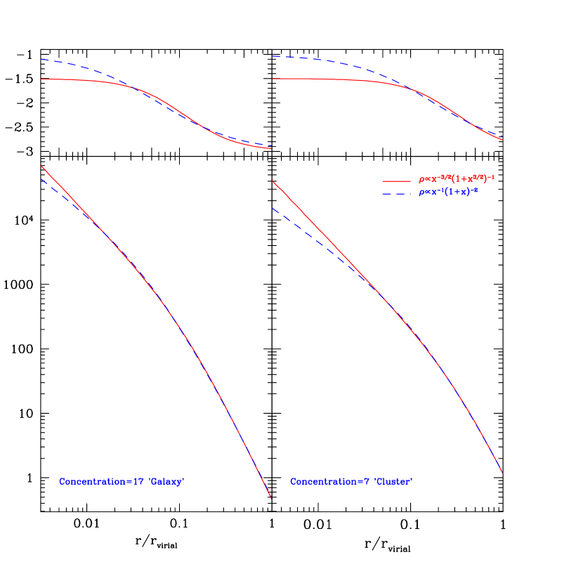
Figure 1: Comparison of the Moore et al. and the NFW profiles. Each profile is normalized to have the same virial mass and the same radius of the maximum circular velocity. Left panels: High concentration halo with concentration typical for small galaxies $C_{\rm NFW}=17$ Right panels: Low concentration halo with concentration typical for clusters of galaxies. The deviations are very small ($<3\%$) for radii $r>1/2r_{s}$. Top panels show the local logarithmic slope of the profiles. Note that for the high concentration halo the slope of the profile is significantly larger than the asymptotic value -1 even at very small radii $r\approx 0.01/r_{\rm vir}$.

3 Properties of Dark Matter Halos

Some properties of halos depend on large-scale environment in which the halos are found. We will call a halo distinct if it is not inside a virial radius of another (larger) halo. Halo is called subhalo, if it is inside of another halo. The number of subhalos depends on the mass resolution – the deeper we go, the more subhalos we will find. Most of the results below are based on a simulation, which was complete to masses down to $10^{11}\mbox{$h^{-1}$M${}_{\odot}$}$ or, equivalently, to the maximum circular velocity of 100 km/s.

Mass and Velocity Distribution functions. Extensive analysis of halo mass and velocity function was done by Sigad et al. (2000) for halos in the $\Lambda$CDM  model. Additional results can also be found in Ghigna et al. (1999); Moore et al. (1999b); Klypin et al. (1999); Gottlöber, Klypin & Kravtsov (1998). Figure 2 compares the mass function of subhalos and distinct halos. The Press-Schechter approximation overestimates the the mass function by a factor of 2 for $M<5\times 10^{12}\mbox{$h^{-1}$M${}_{\odot}$}$ and it somewhat underestimates it at larger masses. More advanced approximation given by Sheth & Tormen is more accurate. On scales below $10^{14}\mbox{$h^{-1}$M${}_{\odot}$}$ the mass function is close to a power law with the slope $\alpha\approx-1.8$. There is no visible difference in the slope for subhalos and for the distinct halos.

Figure 2: Mass function for distinct halos (top) and for subhalos bottom). Raw counts are marked by symbols with error bars. The curves are Schechter-function fits. Press-Schechter (dotted) and Sheth-Tormen (dashed) predictions for distinct halos are also shown. On scales below $10^{14}\mbox{$h^{-1}$M${}_{\odot}$}$ the mass function is close to a power law with the slope $\alpha\approx-1.8$. There is no visible difference in the slope for subhalos and for the distinct halos. (After Sigad et al. (2000))

For each halo one can measure the maximum circular velocity $V_{\rm max}$. In many cases (especially for subhalos) $V_{\rm max}$ is a better measure of how large is the halo. It is also closer related with observed properties of galaxies hosted by halos. Figure 3 presents the velocity distribution function of different types of halos. In addition to distinct halos and subhalos, we show also isolated halos and halos in groups and clusters. Here isolated halos are defined as halos with mass less than $10^{13}\mbox{$h^{-1}$M${}_{\odot}$}$, which are not inside a larger halo and which do not have subhalos more massive than $10^{11}\mbox{$h^{-1}$M${}_{\odot}$}$. The velocity function is approximated by a power law $dn=\Phi_{*}V_{\rm max}^{\beta}dV_{\rm max}$ with the slope $\beta\approx-3.8$ for distinct halos. The slope depends on environment: $\beta\approx-3.1$ for halos in groups and $\beta\approx-4$ for isolated halos. Klypin et al. (1999) and Ghigna et al. (1999) found that the slope $\beta\approx-3.8-4$ of the velocity function extends to much smaller halos with velocities down to 10 km/s.

Figure 3: Velocity functions for isolated halos (squares) and for halos in groups and clusters. Halos with mass less than $10^{13}\mbox{$h^{-1}$M${}_{\odot}$}$ are used for the plots. (After Sigad et al. (2000))

Correlation between characteristic density and radius. The halo density profiles are approximated by the Navarro-Frenk-White profile:

$$\rho=\frac{\rho_{0}}{(r/r_{0})[1+r/r_{0}]^{2}}$$ (1)

Kravtsov et al. (1999) find the correlation between the two parameters of halos $\rho_{0}$ and $r_{s}$. Fifure 4 compares results for the dark matter halos with those for the the dark matter dominated Low Surface Brightness (LSB) galaxies and dwarf galaxies. Halos are consistent with observational data: smaller halos are denser.

Figure 4: Correlation of the characteristic density $\rho_{0}$ and radius $r_{0}$ for the dwarf and LSB galaxies (solid and open circles) and for the dark matter halos (crosses) in different cosmological models. Halos are consistent with observational data: smaller halos are denser. (After Kravtsov et al. (1999))

Correlations between mass, concentration, and redshift. Navarro et al. (1997) argued that the halo profiles have a universal shape in the sense that profile is uniquely defined by virial mass of the halo. Bullock et al. (2000) analyzed concentrations of thousands of halos at different redshifts. To some degree they confirm conclusions of Navarro et al. (1997): halo concentration correlates with its mass. But some significant deviations were also found. There is no one-to-one relation between concentration and mass. It appears the the universal profile should only be treated as a trend: halo concentration does increase as the halo mass decreases, but there are large deviations for individual halos from that “universal” shape. Halos have intrinsic scatter of concentration: at $1\sigma$ level halos with the same mass have $\Delta(\log{c_{\rm vir}})=0.18$ or, equivalently, $\Delta\mbox{$V_{\rm max}$}/\mbox{$V_{\rm max}$}=0.12$.

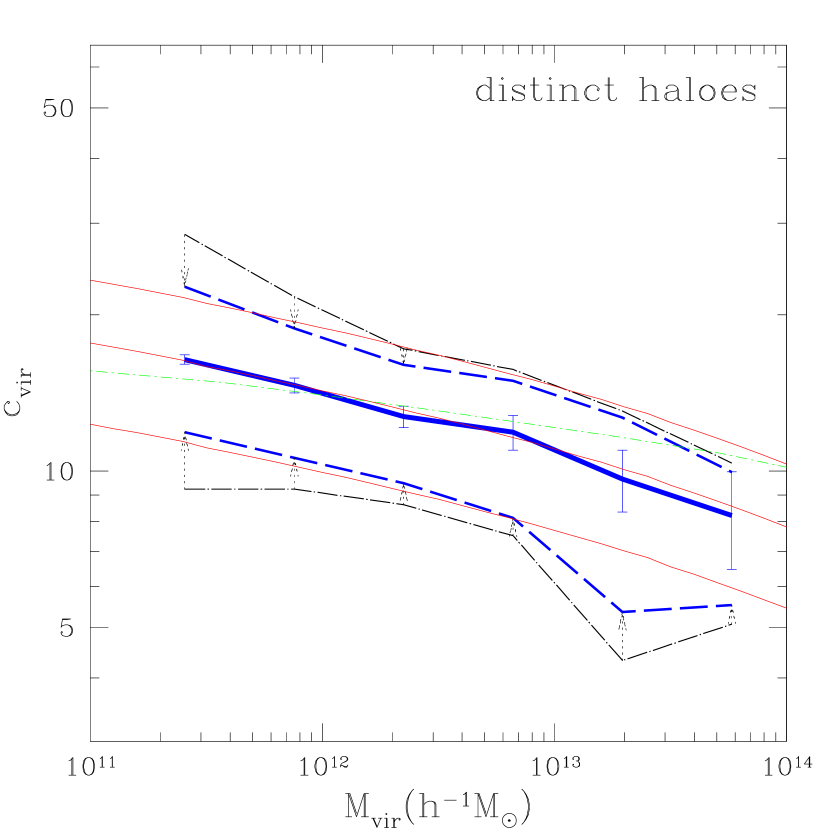
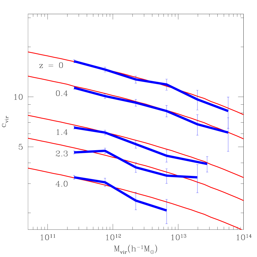
Figure 5: Left Panel Dependence of concentration with mass for distinct halos. The thick solid curve is the median value. The errors are errors of the mean due to sampling. The outer dot-dashed curves encompass 68% of halos in the simulations. The dashed curves and arrows indicate values corrected for the noise in halo profiles.Thin curves are different analytical models. Right Panel Median halo concentration as a function of mass for different redshifts. The thin lines show predictions of an analytical model. (After Bullock et al. (2000)).

Velocity anisotropy. Inside a large halo subhalos or dark matter particles do not move on either circular or radial orbits. Velocity ellipsoid can be measured at each position inside halo. It can be characterized by anisotropy parameter defined as $\beta(r)=1-V^{2}_{\perp}/2V^{2}_{r}$. Here $V^{2}_{\perp}$ is the velocity dispersion perpendicular to the radial direction and $V^{2}_{r}$ is the radial velocity dispersion. For pure radial motions $\beta=1$. For isotropic velocities $\beta=0$. Function $\beta(r)$ was estimated for halos in different cosmological models ( see Colín et al. (1999) for references). By studying 12 rich clusters with many subhalos inside each of them, Colín et al. (1999) found that both the subhalos and dark matter particles can be described by the same anisotropy parameter

$$\beta(r)=0.15+\frac{2x}{x^{2}+4},\quad x=r/r_{\rm vir}$$ (2)

4 Halo profiles: Convergence study

The following results are based on Klypin et al. (2000)

4.1 Numerical simulations

Table 2: Parameters of Halos

	z	$M_{\rm vir}$	$R_{\rm vir}$	$V_{\rm max}$	$N_{\rm part}$	$m_{\rm part}$	Form.res.	$C_{\rm NFW}$	RelEr	RelEr
		$M_{\odot}/h$	kpc/h	km/s		$M_{\odot}/h$	kpc/h		NFW	Moore
(1)	(2)	(3)	(4)	(5)	(6)	(7)	(8)	(9)	(10)	(11)
A1	0	$1.97\cdot 10^{12}$	257	247.0	$1.2\cdot 10^{5}$	$1.6\cdot 10^{7}$	0.23	17.4	0.17	0.20
A2	0	$2.05\cdot 10^{12}$	261	248.5	$1.5\cdot 10^{4}$	$1.3\cdot 10^{8}$	0.91	16.0	0.13	0.16
A3	0	$1.98\cdot 10^{12}$	256	250.5	$1.9\cdot 10^{3}$	$1.1\cdot 10^{9}$	3.66	16.6	0.16	0.10
B	1	$8.5\cdot 10^{11}$	241	195.4	$7.1\cdot 10^{5}$	$1.2\cdot 10^{6}$	0.19	12.3	0.23	0.16
C	1	$6.8\cdot 10^{11}$	208	165.7	$5.0\cdot 10^{5}$	$1.2\cdot 10^{6}$	0.19	11.9	0.37	0.20
D	1	$9.6\cdot 10^{11}$	245	202.4	$7.9\cdot 10^{5}$	$1.2\cdot 10^{6}$	0.19	9.5	0.25	0.60

Using the ART code (Kravtsov, Klypin & Khokhlov, 1997; Kravtsov, 1999), we simulate a flat low-density cosmological model ($\Lambda$CDM) with $\Omega_{0}=1-\Omega_{\Lambda}=0.3$, the Hubble parameter (in units of $100{\rm\ kms^{-1}Mpc^{-1}}$) $h=0.7$, and the spectrum normalization $\sigma_{8}=0.9$. We have run two sets of simulations with $30\mbox{$h^{-1}$Mpc}$ and $25\mbox{$h^{-1}$Mpc}$ computational box. The first simulations were run to the present moment $z=0$. The second set of simulations had higher mass resolution and therefore produced more halos but were run only to $z=1$.

In all of our simulations step in the expansion parameter was chosen to be $\Delta a_{0}=2\times 10^{-3}$ on the zero level of resolution. This gives about 500 steps for an entire run to $z=0$. A test run was done with twice smaller time-step for a halos of comparable mass (but with smaller number of particles) as studied in this paper. We did not find any visible deviations in the halo profile. In the first set of simulations, the highest level of refinement was ten, which corresponds to $500\times 2^{10}\approx 500,000$ time steps at the tenth level. For the second set of simulation, nine levels of refinement were reached which corresponds to $128,000$ steps at the ninth level.

In the following sections we present results for four halos. The first halo ($A$) was the only halo selected for resimulation in the first set of simulations. In this case the selected halo was relatively quiescent at $z=0$ and had no massive neighbors. The halo was located in a long filament bordering a large void. It was about 10 Mpc away from nearest cluster-size halo. After the high-resolution simulation was completed we found that the nearest galaxy-size halo was about 5 Mpc away. The halo had a fairly typical merging history with $M(t)$ track slightly lower than the average mass growth predicted using extended Press-Schechter model. The last major merger event occured at $z\approx 2.5$; at lower redshifts the mass growth (the mass in this time interval has grown by a factor of three) was due to slow and steady mass accretion.

The second set of simulations was done in a different way. In the low resolution run we selected three halos in a well pronounced filament. Two of the halos are neighbors located at about 0.5 Mpc from each other. The third halo was 2 Mpc away from this pair. Thus, the halos were not selected to be too isolated as was the case in the first set of runs. Moreover, the simulation was analyzed at an earlier moment ($z=1$) where halos are more likely to be unrelaxed. Therefore, we consider the halo $A$ from the first set as an example of a rather isolated well relaxed halo. In many respects, this halo is similar to halos simulated by other research groups that used multiple mass resolution techniques. The three halos from the second set of simulations can be viewed as representative of more typical halos, not necessarily well relaxed and located in more crowded environments.

Parameters of the simulated dark matter halos are listed in Table 2. Columns in the table present (1) Halo “name” (halos A₁, A₂, A₃ are the halo A re-simulated times with different resolutions); (2) redshift at which halo was analyzed; (3-5) virial mass, comoving virial radius, and maximum circular velocity. At $z=0$ ($z=1$) the virial radius was estimated as the radius within which the average overdensity of matter is 340 (180) times larger than the mean cosmological density of matter at that redshift; (6) the number of particles within the virial radius; (7) the smallest particle mass in the simulation; (8) formal force resolution achieved in the simulation. As we will show below, convergent results are expected at scales larger than four times the formal resolution; (9) halo concentration as estimated from NFW profile fits to halo density profiles; (10) maximum relative error of the NFW fit: $\rho_{\rm NFW}/\rho_{\rm halo}-1$ (the error was estimated inside $50\mbox{$h^{-1}$kpc}$ radius); (11) the same as in the previous column, but for the fits of profile advocated by Moore et al.

Halo $A$ in the first set of simulations was re-simulated three times with increasing mass resolution. For each simulation, we considered outputs at four time moments in the interval to $z=0-0.03$. Parameters of the halos in these simulations averaged over the four moments are presented in the first three rows of the Table 2. We do not find any systematic change with resolution in the values of halo parameters both on the virial radius scale and around the maximum of the circular velocity ($r=(30-40)\mbox{$h^{-1}$kpc}$).

Left panel in Figure 6 shows the central region of the halo A₁ (see Table 2). This plot is similar to the Fig.1a in Moore et al. (1998) in that all profiles are drawn to the formal force resolution. The straight lines indicate slopes of two power-laws: $\gamma=-1$ and $\gamma=-1.4$. The figure indeed shows that at around 1% of the virial radius the slope is steeper than -1 and the central slope increases as we increase the mass resolution. Moore et al. (1998) interpreted this behavior as evidence that profiles are steeper than predicted by the NFW profile. We also note that the results of our highest resolution run $A_{1}$ are qualitatively consistent with results of Kravtsov et al. (1998). Indeed, if the profiles are considered down to the scale of two formal resolutions, the density profile slope in the very central part of the profile $r\lesssim 0.01r_{\rm vir}$ is close to $\gamma=-0.5$.

The profiles in Figure 6 reflect the density distribution in the cores of simulated halos. However, the interpretation of these profiles is not straightforward because it requires assessment of numerical effects. The formal resolution usually does not even correspond to the scale where the numerical force is fully Newtonian (usually it is still considerably “softer” than the Newtonian value). In the ART code, the interparticle force reaches (on average) the Newtonian value at about two formal resolutions(see Kravtsov et al. 1997). The effects of force resolution can be studied by resimulating the same objects with higher force resolution and comparing the density profiles. Such convergence study was done in Kravtsov et al. (1998) where it was found that for a fixed mass resolution halo density profiles converge at scales above two formal resolutions. Second, local dynamical time for particles moving in the core of a halo is very short. For example, particles on the circular orbit of the radius $1\mbox{$h^{-1}$kpc}$ from the center of halo $A$ makes about 200 revolutions over the Hubble time. Therefore, if the time step is insufficiently small, numerical errors in these regions will tend to grow especially fast. The third possible source of numerical errors is mass resolution. Poor mass resolution in simulations with good force resolution may, for example, lead to two-body effects (e.g., Knebe et al. 2000). Insufficient number of particles may also result in “grainy” potential in halo cores and thereby affect accuracy of orbit integration. In these effects, the mass resolution may be closely inter-related with force resolution.

It is clear thus that in order to make conclusions not affected by numerical errors, one has to determine the range of trustworthy scales using convergence analysis. Right panel in Figure 6 shows that for the halo A simulations the convergence for vastly different mass and force resolution is reached for scales $\gtrsim 4$ formal force resolutions (all profiles in this figure are plotted down to the radius of 4 formal force resolutions). For all resolutions, there are more than 200 particles within the radius of four resolutions from the halo center. For the highest resolution simulation (halo A₁) the convergence is reached at scales $\gtrsim 0.005\mbox{$r_{\rm vir}$}$.

In order to judge which profile provides a better description of the simulated profiles we fitted the NFW and Moore et al. analytic profiles. Figure 7 presents results of the fits and shows that both profiles fit the numerical profile equally well: fractional deviations of the fitted profiles from the numerical one are smaller than 20% over almost three decades in radius. It is clear thus that the fact that numerical profile has slope steeper than $-1$ at the scale of $\sim 0.01\mbox{$r_{\rm vir}$}$ does not mean that good fit of the NFW profile (or even analytic profiles with shallower asymptotic slopes) cannot be obtained.

There is certainly a certain degree of degeneracy in fitting various analytic profile to numerical results. Figure 8 illustrates this further by showing results of fitting profiles (solid lines) of the form $\rho(r)\propto(r/r_{0})^{-\gamma}[1+(r/r_{0})^{\alpha}]^{-(\beta-\alpha)/\gamma}$ to the same (halo $A_{1}$) simulated halo profile shown as solid circles. The legend in each panel indicates the corresponding values of $\alpha$, $\beta$, and $\gamma$ of the fit; the digit in parenthesis indicates whether the parameter was kept fixed ($0$) or not ($1$) during the fit. The right two panels show fits of the NFW and Moore et al. profiles; the bottom left panel shows fit of the profiles used by Jing & Suto (2000). The top left panel shows a fit in which the inner slope was fixed but $\alpha$ and $\beta$ were fit. The figure shows that all four analytic profiles can provide a nice fit to the numerical profile in the whole range $0.005-1\mbox{$r_{\rm vir}$}$.

Figure 6: Left panel Density profiles of halo A simulated with different mass and force resolutions. The profiles are plotted down to the formal force resolution of each simulation.Right panel The profiles plotted down to four formal resolutions. It is clear that for vastly different mass (from 2000 to 120000 particles in the halo) and force (from $3.66\mbox{$h^{-1}$kpc}$ to $0.23\mbox{$h^{-1}$kpc}$) resolutions the convergence is reached at these scales.

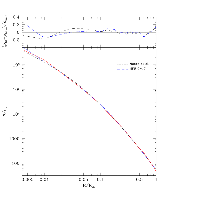
Figure 7: Fits of the NFW and Moore et al. halo profiles to the profile of halo A₁ )bottom panel. The top panel shows fractional deviations of the analytic fits from the numerical profile. Note that both analytic profiles fit numerical profile equally well: fractional deviations are smaller than 20% over almost three decades in radius.

Figure 8: Analytic fits to the density profile of the halo $A_{1}$ (see Table 2) from our set of simulations. The fits are of the form $\rho(r)\propto(r/r_{0})^{-\gamma}[1+(r/r_{0})^{\alpha}]^{-(\beta-\alpha)/\gamma}$. The legend in each panel indicates the corresponding values of $\alpha$, $\beta$, and $\gamma$ of the fit; the digit in parenthesis indicates whether the parameter was kept fixed ($0$) or not ($1$) during the fit. Note that various sets of parameters $\alpha$, $\beta$, $\gamma$ provide equally good fits to the simulated halo profile in the whole range resolved range of scales $\approx 0.005-1\mbox{$r_{\rm vir}$}$. This indicates a large degree of degeneracy in parameters $\alpha$, $\beta$, and $\gamma$

4.2 Halo profiles at $z=1$

As we mentioned in § 4.1, the halo A analyzed in the previous section is somewhat special because it was selected as an isolated relaxed halo. In order to reach unbiased conclusions, in this section we will present analysis of halos from the second set of simulations (halos B, C, and D in Table 2) which were not selected to be relaxed or isolated. Based on the results of convergence study presented in the previous section, we will consider profiles of these halos only at scales above four formal resolutions use results starting only from 4 formal resolutions and not less than 200 particles. Note that these conditions are probably more stringent than necessary because these halos were simulated with $5-7$ times more particles per halo. There is an advantage in analyzing halos at a relatively high redshift. Halos of a given mass will have lower concentration (see Bullock et al. 2000). Lower concentration implies a large scale at which the asymptotic inner slope is reached. Profiles of the high redshift halos should therefore be more useful in discriminating between the analytic models with different inner slopes.

We found that substantial substructure is present inside the virial radius in all three halos. Figure 9 shows profiles of these halos at $z=1$. There profiles are not as smooth as that of halo A₁ due to the substructure. Note that bumps and depressions visible in the profiles cannot are significantly larger amplitude than the shot noise. Halo $C$ appeared to be the most relaxed of the three halos. This halo had the last major merger somewhat earlier than the other two. Halo $D$ had a major merger event at $z\approx 2$. Remnant of the merger are still visible as a hump at radii around $100\mbox{$h^{-1}$kpc}$. The non-uniformities of profiles cause by substructure may substantially bias analytic fits to the entire range of scales below the virial radius. Therefore, we used only the central, presumably more relaxed, regions in the analytic fits: $r<50\mbox{$h^{-1}$kpc}$ for halo D and $r<100\mbox{$h^{-1}$kpc}$ for halos B and C (fits using only central $50\mbox{$h^{-1}$kpc}$ did not change results).

The best fit parameters were obtained by minimizing the maximum fractional deviation of the fit: ${\rm max}({\rm abs}(\log\rho_{\rm fit})-\log\rho_{\rm halo})$. Minimizing the sum of squares of deviations ($\chi^{2}$), as is often done, can result in larger errors at small radii with the false impression that the fit fails because it has a wrong central slope. The fit that minimizes maximum deviations, improves the NFW fit for points in the range of radii $(5-20)\mbox{$h^{-1}$kpc}$, where the NFW fit would appear to be below the data points if the fit was done by the $\chi^{2}$ minimization. This improvement comes at the expense of few points around $1\mbox{$h^{-1}$kpc}$. For example, if we fit halo B by using $\chi^{2}$ minimization, the concentration decreases from 12.3 (see Table 2) to 11.8 We also made a fit for halo B assuming even more stringent limits on the effects of numerical resolution. By minimizing the maximum deviation we fitted the halo starting at six times the formal resolution. Inside this radius there were about 900 particles. Resulting parameters of the fit were close to those in Table 2: $C_{\rm NFW}=11.8$, and maximum error of the NFW fit was 17%.

We found that the errors in the Moore et al. fits were systematically smaller than those of the NFW fits, though the differences were not dramatic. Moore et al. fit failed for halo $D$. It formally gave very small errors, but this was done for a fit with unreasonably small concentration $C=2$. When we constrained the approximation to have about twice larger concentration as compared with the best NFW fit, we were able to obtain a reasonable fit (this fit is shown in Figure 9). Nevertheless, the central part was fit poorly in this case.

Our analysis therefore failed to determine which analytic profile provides a better description of the density distribution in simulated halos. Despite the larger number of particles per halo and lower concentrations of halos, results are still inconclusive. Moore at al. profile is a better fit to the profile of halo C; the NFW profile is a better fit to the central part of halo D. Halo B represents an intermediate case where both profiles provide equally good fits (similar to the analysis of halo A).

Note that there seem to be real deviations in parameters of halos of the same mass. Halos B and D have the same virial radii and nearly the same circular velocities, yet their concentrations are different by 30%. We find the same differences in estimates of $C_{1/5}$ concentrations, which do not depend on specifics of an analytic fit. The central slope at around $1\mbox{kpc}$ also changes from halo to halo.

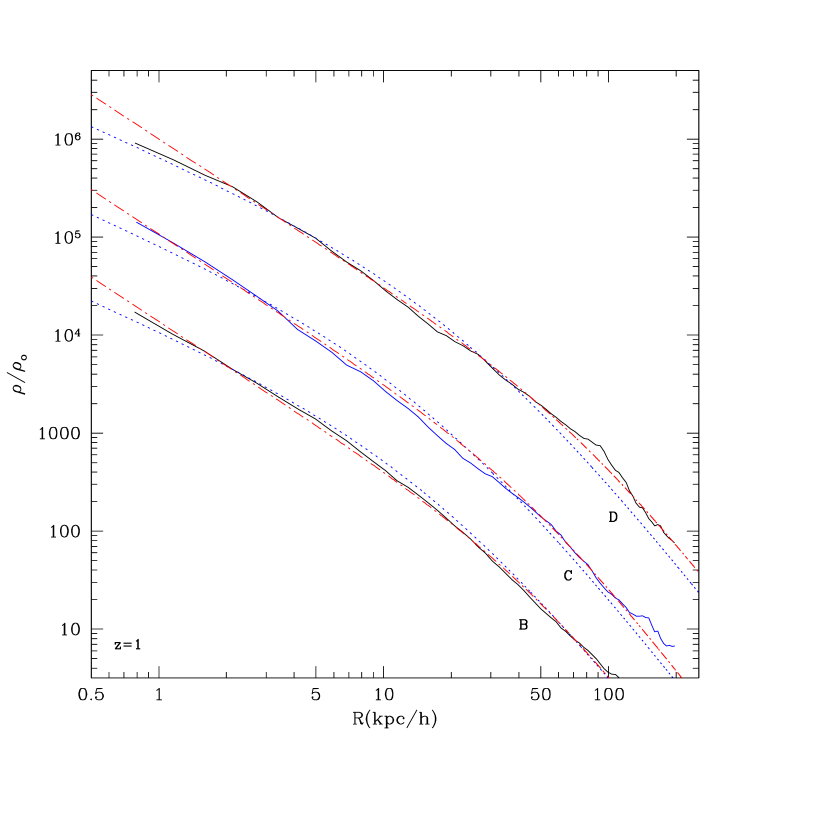
Figure 9: Profiles of halos B, C, D at $z=1$. Profiles of halos C and D were offset downwards by factors of 10 and 100 for clarity. Solid curves show simulated profiles, while dotted and dot-dashed curves show the NFW and Moore et al. fits, respectively. The halo profiles in simulations are plotted down to four formal resolution. Each halo had more than 200 particles inside the smallest plotted scale.

5 Summary

We run a series of simulations with vastly different mass and force resolution with the goal of studying the shape of the dark matter halo profile in central parts of galaxy-size halos. We use a modified version of the ART code, which is capable of handling particles with different masses, variable force, and time resolution. In runs with the highest resolution, the code achieved (formal) dynamical range of $2^{17}=131,072$ with 500,000 steps for particles at highest level of resolution.

Our conclusions regarding the convergence of the profiles differ from those of Moore et al. (1997). If we take into account only radii, at which we believe numerical effects (the force resolution, the resolution of initial perturbations, and the two-body scattering) are small, then we find that the slope and the amplitude of the density do not change when we change the force and mass resolution. This result is consistent with what was found in simulations of the “Santa Barbara” cluster (Frenk et al., 1999): at a fixed resolved scale results do not change as the resolution increases. For the ART code the results converged at 4 times the formal force resolution and more than 200 particles. These limits of convergence very likely depend on particular code used and on the duration of integration.

We reproduce results of Moore et al. regarding the convergence and results of Kravtsov et al. (1998) regarding shallow central profiles, but only when we consider points inside unresolved scales. We conclude that those results followed from overly optimistic interpretation of numerical accuracy of simulations.

For the galaxy-size halos considered in this paper with masses $M_{\rm vir}=7\times 10^{11}\mbox{$h^{-1}$M${}_{\odot}$}-2\times 10^{12}\mbox{$h^{-1}$M${}_{\odot}$}$ and concentrations $C=9-17$ both the NFW profile $\rho\propto r^{-1}(1+r)^{-2}$ and the Moore et al. profile $\rho\propto r^{-1.5}(1+r^{1.5})^{-1}$ give good fits with accuracy about 10% for radii not smaller than 1% of the virial radius. None of the profiles is significantly better then the other.

Halos with the same mass may have different profiles. No matter what profile is used – NFW or Moore et al. – there is no universal profile: just halo mass does not yet define the density profile. Nevertheless, the universal profile is extremely useful notion which should be interpreted as the general trend $C(M)$ of halos with larger mass to have lower concentration. Deviations from the general $C(M)$ are real and significant (Bullock et al., 2000). It is not yet clear, but seems very likely that the central slopes of halos also have real fluctuations. The fluctuations in the concentration and the central slopes are important for interpretation of the central parts of rotation curves.

References

- Binney & Tremaine (1987) Binney, J., & Tremaine, S. 1987, Galactic Dynamics, Princeton: Princeton Univ. Press
- Bullock et al. (2000) Bullock, J.S., Kolatt, T.S., Sigad, Y., Somerville, R.S., Kravtsov, A.V., Klypin, A., Primack, J.P., Dekel, A. 2000, MNRAS submitted ( astro-ph/9908159)
- Bullock, Kravtsov & Weinberg (2000) Bullock, J.S., Kravtsov, A.V., & Weinberg, D.H. 2000, ApJ in press (astro-ph/0002214)
- Colín et al. (1999) Colín, P., Klypin, A.A., Kravtsov, A.V., & A.M. Khokhlov. 1999, ApJ in press (astro-ph/9809202)
- Gottlöber, Klypin & Kravtsov (1998) Gottlöber, S., Klypin, A., & Kravtsov, A.V. 1998, in ASP Conference Series Vol. 176, 1999, ”Observational Cosmology: The Development of Galaxy Systems”, eds.: G. Giuricin, M. Mezetti, P. Salucci, p. 418
- Flores & Primack (1994) Flores, R.A., & Primack, J.R. 1994, ApJ 427, L1
- Ghigna et al. (1998) Ghigna, S., Moore, B., Governato, F., Lake, G., Quinn, T., Stadel, J. 1998, MNRAS, 300, 146
- Ghigna et al. (1999) Ghigna, S., Moore, B., Governato, F., Lake, G., Quinn, T., Stadel, J. 1999, ApJ submitted (astro-ph/9910166)
- Jing (1999) Jing, Y.P. 1999, ApJ submitted (astro-ph/9901340)
- Jing & Suto (2000) Jing, Y.P. & Suto, Y. 2000, ApJ 529, L69
- Kauffmann et al. (1993) Kauffmann, G., White, S.D.M., & Guiderdoni, B. 1993, MNRAS 264, 201
- Klypin et al. (1998) Klypin, A., Gotlöber, S., Kravtsov, A.V., Khokhlov, A.. 1998, ApJ, 516, 530 (KGKK)
- Klypin et al. (1999) Klypin, A., Kravtsov, A.V., Valenzuela, O., & Prada, F. 1999, ApJ, 522, 82
- Klypin et al. (2000) Klypin, A., Kravtsov, A.V., Bullock, J.S., & Primack, J.P. 2000, in preparation
- Knebe et al. (2000) Knebe A., Kravtsov, A.V., Gottlöber, S., & Klypin A. 2000, MNRAS in press ( astro-ph/9912257)
- Kravtsov (1999) Kravtsov, A.V. 1999, Ph.D. Thesis, New Mexico State University
- Kravtsov et al. (1999) Kravtsov, A.V., Klypin, A., Bullock, J.S., & Primack, J.P. 1999, ApJ 502, 48
- Kravtsov & Klypin (1999) Kravtsov, A.V., & Klypin, A. 1999, ApJ 520, 437
- Kravtsov, Klypin & Khokhlov (1997) Kravtsov, A.V., Klypin, A., & Khokhlov, A.M. 1997, ApJS 111, 73
- Moore et al. (1998) Moore, B., Governato, F., Quinn, T., Stadel, J., Lake, G. 1998, ApJ 499, L5
- Moore et al. (1999a) Moore, B., Quinn, T., Governato, F., Stadel, J., Lake, G. 1999, MNRAS 310, 1147
- Moore et al. (1999b) Moore, B., Ghigna, S., Governato, F., Lake, G., Quinn, T., Stadel, J., & Tozzi, P. 1999, ApJL, in press. (astro-ph/9907411)
- Moore (1994) Moore, B. 1994, Nature 370, 629
- Navarro et al. (1996) Navarro, J.F., Frenk, C.S., & White, S.D.M. 1996, ApJ 462, 563
- Navarro et al. (1997) Navarro, J.F., Frenk, C.S., & White, S.D.M. 1997, ApJ 490, 493
- Navarro & Steinmetz (2000) Navarro, J.F., & Steinmetz, M. 2000, ApJ 528, 607
- Navarro & Swaters (2000) Navarro, J.F., & Swaters, R.A. 2000, in preparation
- Sigad et al. (2000) Sigad, Y., Kolatt, T.S., Bullock, J.S., Kravtsov, A.V., Klypin, A., Primack, J.R., & Dekel, A. 2000, in preparation
- Swaters et al. (2000) Swaters, R.A., Madore, B.F., Trewhella, M. 2000, ApJ 531, L107
- van den Bosch et al. (2000) van den Bosch, F.C., Robertson, B.E., Dalcanton, J.J., de Blok W.J.G. 2000, AJ 119, 1579
- van den Bosch (2000) van den Bosch, F.C. 2000, in preparation