The Spatial and Kinematic Distributions of Cluster Galaxies in a $\Lambda$CDM Universe – Comparison with Observations

Abstract

We combine dissipationless N-body simulations and semi-analytic models of galaxy formation to study the spatial and kinematic distributions of cluster galaxies in a $\Lambda$CDM cosmology. We investigate how the star formation rates, colours and morphologies of galaxies vary as a function of distance from the cluster centre and compare our results with the CNOC1 survey of galaxies from 15 X–ray luminous clusters in the redshift range $0.18<z<0.55$. In our model, gas no longer cools onto galaxies after they fall into the cluster and as a result, their star formation rates decline on timescales of $\sim 1-2$ Gyr. Galaxies in cluster cores have lower star formation rates and redder colours than galaxies in the outer regions because they were accreted earlier. Our colour and star formation gradients agree with those derived from the data. The difference in velocity dispersions between red and blue galaxies observed in the CNOC1 clusters is also well reproduced by the model. We assume that the morphologies of cluster galaxies are determined solely by their merging histories. A merger between two equal mass galaxies produces a bulge and subsequent cooling of gas results in the formation of a new disk. Morphology gradients in clusters arise naturally, with the fraction of bulge-dominated galaxies highest in cluster cores. The fraction of bulge-dominated galaxies inside the virial radius depends on the mass of the cluster, but is independent of redshift for clusters of fixed mass. Galaxy colours and star formation rates do not depend on cluster mass. We compare the distributions of galaxies in our simulations as a function of bulge-to-disk ratio and as a function of projected clustercentric radius to those derived from the CNOC1 sample. We find excellent agreement for bulge-dominated galaxies. The simulated clusters contain too few galaxies of intermediate bulge-to-disk ratio, suggesting that additional processes may influence the morphological evolution of disk-dominated galaxies in clusters. Although the properties of the cluster galaxies in our model agree extremely well with the data, the same is not true of field galaxies. Both the star formation rates and the colours of bright field galaxies appear to evolve much more strongly from redshift 0.2 to 0.4 in the CNOC1 field sample than in our simulations.

1 Introduction

In recent years, there has been a huge observational effort aimed at understanding the evolution of galaxy populations in clusters. High resolution images from the Hubble Space Telescope have been used to study the morphologies of cluster galaxies and to quantify the incidence of interacting or disturbed systems out to $z\sim 1$ (see for example Oemler et al 1997; Lubin et al 1998) . Multi-object spectroscopy has been used to confirm cluster membership and to study the star formation histories and kinematics of cluster galaxies (e.g. Dressler et al 1999; Poggianti et al 1999). Some recent studies (e.g. Abraham et al 1996; Balogh et al 1999, Van Dokkum et al 1998) have focused on the observed trends in star formation and morphology as a function of position within the cluster. These studies demonstrate that there is a smooth transition from a blue, disk-dominated population of galaxies in the outskirts of clusters to a red, bulge-dominated population in the cluster cores. In spite of this wealth of new data, the physical processes responsible for driving the transformation of galaxies in groups and clusters remain poorly understood. Galaxy-galaxy interactions and mergers (Lavery & Henry 1988), tidal disruption (Byrd & Valtonen 1990), interactions with the intracluster medium (Farouki & Shapiro 1980; Abadi, Moore & Bower 1999) and repeated high-speed galaxy encounters with the cluster potential (“harassment”; Moore et al 1996) are all popular explanations of some of the properties of the blue galaxies seen in intermediate redshift clusters (Butcher & Oemler 1978). In order to understand trends in galaxy properties as a function of environment and of redshift, it is necessary to consider both the physical processes that affect galaxies in dense environments and the assembly of the cluster itself. The formation of clusters has traditionally been studied in one of two ways: 1) using methods based on the extended Press-Schechter (EPS) theory (Bower 1991; Bond et al 1991), 2) using N-body simulations of gravitational clustering.

Kauffmann (1995 a,b) used the EPS approach to show that the evolutionary history is different for a rich cluster seen at high redshift than for a cluster of the same mass observed today. When simplified prescriptions for gas cooling, star formation, supernova feedback and galaxy-galaxy merging were included in the models, the fraction of blue star-forming galaxies in rich clusters was shown to increase with redshift. The best fit to the data was obtained for a high-density CDM cosmology. Because clusters evolve more slowly in a low-density Universe, the low-$\Omega$ models produced a much weaker trend in blue fraction with redshift, in apparent contradiction with the observations. The disadvantage of the EPS approach is that it is not possible to model the spatial distribution of galaxies within rich clusters. The models do not follow substructure within individual dark matter halos. It is thus not possible to study whether the observed radial gradients in clusters arise because processes such as ram-pressure stripping operate more efficiently in cluster cores, or because galaxies in the central regions were accreted at an earlier epoch than galaxies on the outside.

Evrard, Silk & Szalay (1990) modelled the spatial distribution of galaxies in an N-body simulation of a cluster by associating galaxies with peaks in the initial density field. They proposed that elliptical galaxies were associated with the highest peaks and that spiral galaxies were associated with smaller peaks and demonstrated that they could obtain a morphology-density relation in reasonable agreement with observations. The disadvantage of this study was that galaxy formation was treated in an extremely simplistic way and it was not possible to make close contact with observational data.

In this paper, we study the evolution of galaxies in clusters using an N-body simulation in which the formation and evolution of galaxies are followed using prescriptions taken directly from semi-analytic models. We focus on how the properties of galaxies vary as a function of position in the clusters and how these trends evolve with redshift. The techniques used for constructing dark matter halo merger trees from the simulation and the recipes used for cooling, star formation, feedback, and galaxy-galaxy merging were described in Kauffmann et al (1999a, hereafter KCDW). This paper also described the global properties of galaxies at $z=0$ including their luminosity functions and two-point correlation functions.

In previous papers (KCDW; Kauffmann et al 1999b; Diaferio et al. 1999), we have explored two different cosmologies: a high-density CDM model ($\tau$CDM) with $\Omega=1$, $\sigma_{8}=0.6$ and $H_{0}=50$ km s^-1 Mpc^-1, and a low-density model with $\Omega=0.3$, $\Lambda=0.7$ $\sigma_{8}=0.9$ and $H_{0}=70$ km s^-1 Mpc^-1 ($\Lambda$CDM). We found that the $\tau$CDM model consistently failed to fit the observations as well as the $\Lambda$CDM model. In particular, $\tau$CDM produced a field galaxy luminosity function with too many very bright galaxies (Kauffmann et al 1999a) and was unable to reproduce the topology of the large scale galaxy distribution (Schmalzing and Diaferio 2000). In this paper, we only consider the more successful $\Lambda$CDM model. All quantities are for $H_{0}=70$ km s^-1 Mpc^-1.

The simulation volume is 14000 km s^-1 on a side and contains $\sim 140$ clusters with masses greater than $10^{14}M_{\odot}$ at $z=0$. The clusters contain between 5000 and 80000 dark matter particles. As discussed in KCDW, the B-band luminosities of galaxies in the simulation can be reliably determined down to $\sim 1.5$ magnitudes below $L_{*}$. Because the morphologies of galaxies depend on their detailed merging histories, galaxy types can only be determined for objects brighter than $\sim L_{*}$. To obtain reasonable statistics, we stack all the clusters in the simulation and rescale the clustercentric distances by dividing by $R_{200}$, the virial radius of the cluster. This approach follows the one adopted by Yee et al (1996) and Balogh et al (1997,1998,1999) in a series of papers analyzing the observed radial trends in clusters in the CNOC1 survey. Where explicit comparisons with observational data are made, we analyze galaxy properties as a function of projected clustercentric distance $R_{proj}$ and exclude galaxies with large velocity differences from the central cluster galaxy. This will be discussed in more detail in section 4.

In section 2, we discuss those aspects of our model that influence the evolution of cluster galaxies. Section 3 summarizes the properties of the simulated clusters. The CNOC1 cluster sample is discussed in section 4. Results on the cluster luminosity function, star formation gradients, colour gradients, morphology gradients and the kinematics of cluster galaxies are presented in sections 5-9. Finally, we summarize our results in section 10.

2 Model assumptions that influence the evolution of cluster galaxies

In this section, we review the processes that influence the evolution of galaxies in clusters in our model.

1. Gas supply and star formation. As discussed in KCDW, the star formation rate in a galaxy is regulated by the rate at which gas cools from the surrounding hot halo and the rate at which supernovae eject cold gas out of the galaxy. When a galaxy is accreted by a more massive group or cluster, it loses its supply of infalling cold gas. Its star formation rate then declines as its existing reservoir of cold gas is used up. The time taken for a blue, star-forming galaxy to exhaust its fuel supply and become red, depends on the assumed star formation timescale. In KCDW we adopted the empirically-motivated star formation law of Kennicutt (1998), which has the form $\dot{M}_{*}=\alpha M_{cold}/t_{dyn}$, where $M_{cold}$ is the mass of cold gas left in the galaxy and $t_{dyn}$ is the dynamical time of the galaxy. The dynamical time of the galaxy is defined when the galaxy was last a central galaxy in a halo, and is given by $t_{dyn}=0.1R_{200}/V_{c}$, where $R_{200}$ and $V_{c}$ are the virial radius and circular velocity of the surrounding halo. The parameter $\alpha$, which controls the efficiency of star formation, was chosen to obtain a cold gas mass of $\sim 8\times 10^{9}M_{\odot}$ for a Milky Way–type galaxy at the present day and has a value $\sim 0.1$. This means that a Milky–Way galaxy in a halo with circular velocity $220$ km s^-1 and virial radius $0.4$ Mpc, will run out of cold gas $\sim 1.5$ Gyr after being accreted by a more massive halo. Note that this calculation of the gas consumption timescale neglects the effects of recycling due to mass loss and supernova ejecta, which may increase it by a factor of 1.5-3, depending upon the assumed IMF (Kennicutt, Tamblyn & Congdon 1994). However, it is also possible that ram-pressure stripping may accelerate the rate at which the gas is removed from galaxies (Abadi et al 1999).

   As shown by Kauffmann & Haehnelt (2000), if $\alpha$ is a constant independent of redshift, the ratio of gas mass to stellar mass in galaxies evolves weakly with redshift. In order to reproduce the observed increase in the total mass of cold gas in the Universe inferred from damped Lyman-alpha systems and to explain the strong increase in the space density of quasars and starburst galaxies from the present day to $z\sim 2$ Kauffmann & Haehnelt adopted a redshift-dependent $\alpha$ of the form $\alpha\propto(1+z)^{-1.5}$. In this case, the fraction of gas converted into stars per dynamical time is lower for high redshift galaxies, so galaxies falling into clusters at high redshift will take longer to exhaust their cold gas reservoirs. Somerville, Primack & Faber (2000) showed that the same star formation law could reproduce the observed evolution of cold gas in damped systems and the properties of Lyman-break galaxies at $z\sim 3$.

   Figure 1 compares the evolution of the gas fractions in field and cluster galaxies for the two star formation prescriptions. If $\alpha$ is constant, the mean ratio of gas to stars in galaxies more massive than $3\times 10^{10}M_{\odot}$ increases by a factor $\sim 2$ from $z=0$ to $z=1$. If $\alpha\propto(1+z)^{-1.5}$, this ratio increases by a factor $\sim 10$ over the same redshift interval. A similar effect is seen in clusters, where the gas-to-star ratios of galaxies are typically a factor of 10 lower than in the field.

   We have explored both star formation laws in this analysis. At the relatively low redshifts of the CNOC1 cluster sample ($0.18<z<0.55$), there is no observationally discernable difference in the star formation rates or colours of cluster galaxies for the two prescriptions. On the other hand, an evolving $\alpha$ results in slightly stronger evolution of the star formation rates of bright field galaxies and is in better agreement with the CNOC1 field sample, so we adopt $\alpha\propto(1+z)^{-1.5}$ as the fiducial model in this paper.

   

   Figure 1: The evolution of the mean ratio of gas mass to stellar mass for galaxies more massive than $3\times 10^{10}M_{\odot}$ in clusters and in the field. The dashed line is for the model with constant $\alpha$ and the solid line is for the model with $\alpha\propto(1+z)^{-1.5}$.

2. Definition of the cluster boundary As described in KCDW, the clusters in our model are selected using a friends-of-friends group-finding algorithm with a linking length $b=0.2$. This means that clusters are defined at an overdensity of $\sim 200$ times the background density at each redshift. A galaxy is said to have been “accreted” by a cluster if it is included in the list of particles that are linked together by the groupfinder. After a galaxy has been accreted, no further cooling of gas onto the galaxy takes place and its star formation rate declines on a timescale that is short compared to the Hubble time. Note that the same thing occurs for galaxies that “escape” temporarily and are not included within the boundary of any halo. Balogh, Navarro & Morris (2000) noted that this occurred quite frequently in the simulations they studied. We note that in their study, “galaxies” were chosen to be a random subset of the particles in the cluster at the end of the simulation, rather than the most-bound particles of the cluster progenitors at high redshift.

   As a result of our approach, a fairly sharp transition occurs at the cluster boundary from a gas-rich, star-forming population of “field” galaxies on the outside to a gas-poor, red population of cluster galaxies on the inside. The cluster boundary lies at a distance of $\sim 1.5-2R_{200}$ from the cluster centre in our $\Lambda$CDM model (Recall that $R_{200}$ is defined relative to the critical density). A more physically realistic treatment of the accretion process would consider how the hot gas surrounding infalling galaxies is shock-heated and tidally stripped from their halos.

3. Merging and morphology. In our model, the morphologies of cluster galaxies are determined by the rate at which they merge and this is in turn set by the merging history of the dark matter component of the cluster. High resolution N-body simulations have shown that if a dark matter satellite falls into a larger halo, the satellite can preserve its identity for some time (e.g. Klypin et al 1999). Smaller satellites may survive for a long time, whereas larger satellites quickly sink to the centre of the halo and merge with the central mass concentration. Since our simulations do not have sufficient resolution to follow the orbits of individual satellites, we have modelled the rate at which dynamical friction causes a satellite halo of given mass to sink to the centre of the larger halo and merge (see KCDW). Detailed comparisons of the simple analytic formula with N-body simulations have shown that on average this treatment provides a reasonably accurate description of merging timescales (Navarro, Frenk & White 1995; Tormen, Diaferio & Syer 1998; van den Bosch 1999; Springel et al 2000). However, some of the most massive satellites take significantly longer to merge than predicted by the simple formula and this has a significant effect on the mass distribution of the brightest galaxies in the clusters (Springel et al 2000).

   If two galaxies of roughly equal mass merge, the remnant is classified as a “bulge”. The stars in the two galaxies are combined and all the cold gas is transformed into stars in a burst lasting $10^{8}$ years. Further cooling leads to the formation of a new disk component. We have made morphological classifications according to the B-band bulge-to-disk ratios of the galaxies in the simulation. Following Balogh et al (1998), we split our sample into three classes: a bulge-dominated class (B), a disk-dominated class (D) and an intermediate class (Int). We choose the boundaries between the classes so as to reproduce the fraction of field galaxies in each class in the CNOC1 data (see figure 17). Bulge-dominated galaxies then have $B/T>0.4$, disk-dominated galaxies have $B/T<0.2$ and the intermediate class has $0.2<B/T<0.4$. (In the CNOC1 data, the corresponding divisions are at $B/T>0.7$ (B), $B/T<0.4$ (D) and, $0.4<B/T<0.7$ (Int) in the $r$-band (see section 4).)

   In our models, satellite galaxies merge only with the central galaxy of the halo. We do not consider the effect of collisions or close encounters between satellites. Springel et al (2000) have found that in high resolution N-body simulations of cluster formation, mergers between satellites are relatively rare (only one in twenty mergers took place between two satellite halos, rather than a satellite and the central halo). On the other hand, the rate of close enounters is high (Tormen, Diaferio & Syer 1998; Kolatt et al 1999) and may be sufficient to explain the observed incidence of blue galaxies with disturbed morphologies in rich clusters at $z\sim 0.4$. Moore at al (1999) have demonstrated that these close encounters may transform low surface brightness disk galaxies into dwarf spheroidals and high surface brightness disks into S0s.

   In our models, bulge-dominated galaxies in clusters are formed by mergers occurring in smaller groups that are later accreted by the cluster. The only galaxy affected by mergers in the cluster itself is the central object, which grows steadily in mass by accreting smaller satellites.

4. Positions of galaxies within the cluster: a reflection of incomplete violent relaxation. As discussed in KCDW, the galaxy formed from gas cooling in a dark matter halo is assigned the index of the most bound particle in that halo. The galaxy is always identified with the same particle, even after it is accreted by a larger group or cluster.

   High-resolution N-body simulations show that the dense cores of dark matter halos often survive after they are accreted by a larger system , even after many crossing times. Springel et al (2000) have developed methods of picking out surviving “subhalos” orbiting within a larger halo and have studied how the subhalos are tidally stripped over time. Subhalos were studied down to a threshold of 10 particles. In 90% of cases, surviving subhalos still contain the most-bound particle identified before the halo was accreted. This result is independent of the resolution of the simulation and it indicates that our technique of using the most-bound particle to mark the positions of galaxies within clusters is robust, particularly for the galaxies with luminosities $>L_{*}$, which always form in dark matter halos of at least 100 particles in our simulations.

   It should be noted that radial trends in galaxy clusters cannot be studied using the simplified procedures for assigning galaxies to halos adopted by Kauffmann, Nusser & Steinmetz (1997) or Benson et al (2000). These authors do not follow the merging histories of the halos in the simulations and simply assign galaxies to a random subset of the halo particles.

5. Spatial bias and the properties of galaxies in the vicinity of clusters. Clusters and rich groups correspond to high peaks in the initial field of density fluctuations and are consequently more highly clustered than dark matter halos of lower mass (Bardeen et al 1986). As a result of this bias, the properties of galaxies in the vicinity of clusters will not be the same as the properties of galaxies in the field. Our procedure of following the formation and evolution of galaxies in the halos defined by the dark matter simulation means that these spatial bias effects are automatically taken into account.

In summary, we have made a set of extremely simple assumptions about the gas physical processes operating within clusters. The true situation is undoubtedly more complicated. Our intention is to concentrate on the radial trends induced by the assembly of the dark matter component of the cluster. If these trends disagree with the observations, we may then learn something about additional physical processes at work in the cluster.

3 The cluster sample in the simulations

We have selected dark matter halos with virial masses $M_{200}\geq 10^{14}M_{\odot}$ at a series of different redshifts. $M_{200}$ is the mass inside $R_{200}$, the radius within which the mass overdensity is 200 times the critical density. The mass distribution of the objects in our sample is shown at a series of redshifts in Fig. 2. Although there are three clusters at z=0 with masses comparable to the Coma cluster ($\geq 10^{15}M_{\odot}$), by z=0.8 the most massive clusters in the simulation volume are more comparable to Virgo. Our sample of high-redshift clusters is therefore not strictly comparable to samples such CNOC1, which include only the most X-ray luminous systems in a substantially larger volume of the Universe. The CNOC1 clusters range from $3.4\times 10^{14}M_{\odot}$ to $4.3\times 10^{15}M_{\odot}$, with a median mass of $1\times 10^{15}M_{\odot}$. In this paper we will attempt to indicate whether or not our results depend on cluster selection by studying how cluster galaxy properties vary as a function of cluster mass in our model.

Cluster galaxies are identified in one of two ways: 1) We use the galaxy positions from the simulations to study the properties of galaxies as a function of physical radius from the cluster centre. 2) We study galaxy properties as a function of two-dimensional projected radius from the central cluster galaxy. In this case, we exclude galaxies with large velocity differences from the central cluster galaxy in exactly the same way as in the observations (see section 4).

Figure 2: The number of clusters in our samples as a function of the logarithm of the virial mass in units of $M_{\odot}$.

4 The CNOC1 cluster sample

The CNOC 1 cluster sample consists of fifteen X–ray luminous clusters in the redshift range $0.18<z<0.55$. Full details of the survey are given in Yee, Ellingson & Carlberg (1996).

Star formation rates for the galaxies were determined from measurements of the equivalent width of the [OII]$\lambda$3727 emission line ($W_{\circ}(OII)$) as described in Balogh et al. (1998), using the calibration of Barbaro & Poggianti (1997). We add a small amount (0.04 h^-2 M_⊙ yr^-1) to the measured rates to compensate for the fact that the $W_{\circ}(OII)$ index is slightly negative in the absence of any emission. The statistical uncertainty in derived star formation rates is typically $\sim$0.2 h^-2 M_⊙ yr^-1. However, there are many systematic uncertainties in the conversion of $W_{\circ}(OII)$ to a star formation rate, as discussed for example by Kennicutt (1998). For this reason, we choose to concentrate on relative star formation rates (for example by comparing cluster and field galaxies), rather than absolute ones.

Morphological parameters for the $r$–band multi-object spectrograph (MOS) images were measured by fitting two dimensional exponential disk and $R^{1/4}$ law profiles to the symmetrized components of the light distribution, as described in Schade et al. (1996a, 1996b). The images are symmetrized to minimize the effects of nearby companions and asymmetric structure, and a $\chi^{2}$ minimization procedure is applied to the models, convolved with the image point spread function, to obtain best fit values of the galaxy size, surface brightness and fractional bulge luminosity (bulge–to–total, or B/T ratio). Simulations show that the B/T measurements are reliable to within about 20% for images of this quality (Schade et al 1996a,b). These measurements are the same as used in Balogh et al (1998).

A proper consideration of selection effects is important, because spectra are not obtained for all the galaxies that were observed photometrically. We correct for these effects using the statistical weights discussed in detail in Yee et al. (1996). The main selection criterion is apparent magnitude; a smaller fraction of faint galaxies are observed spectroscopically, relative to brighter galaxies. The magnitude weight $W_{m}$ compensates for this effect. A second order, geometric weight $W_{xy}$ is computed which compensates for effects such as the undersampling of denser regions, and vignetting near the corners of the chip. Finally, a color weight $W_{c}$ is computed to account for the fact that bluer galaxies are more likely to show emission lines, thus facilitating redshift determination. This is a small effect and we have checked that the inclusion of this weight does not significantly affect any of the results discussed in the present paper. Both $W_{xy}$ and $W_{c}$ are normalized so that their mean is 1.0 for the full sample. In all of our analyses, each galaxy in our sample is weighted by $W_{\rm spec}=W_{m}\times W_{xy}\times W_{c}$ to correct for these selection effects in a statistical manner.

Gunn $g$ and $r$ photometry from the MOS images are available; the photometric uncertainties in these measurements at the spectroscopic limit are about $\sim 0.1$ mag. Absolute $r$ magnitudes ($M_{r}$) are calculated from the photometry for our adopted cosmology ($\Omega=0.3$, $\Lambda=0.7$) and k–corrections are made based on the g-r colors and the model spectral energy distributions of Coleman, Wu & Weedman (1980), convolved with the filter response function, for four, non–evolving spectral types (E/S0, Sbc, Scd and Im). We chose an absolute magnitude limit of $r=-19.3+5\log{h}$, which corresponds to $M_{R}=-20.5$ for $h=0.7$, assuming $r-M_{R}\approx 0.45$ (Fukugita et al. 1995). This magnitude limit is chosen because it correponds to the faintest galaxies for which we can accurately model both star formation rates and morphologies in the simulation. Rest frame $(g-r)_{\circ}$ colours are computed from the colour–redshift relations in Patton et al. (1997), which are fits to the colour k–corrections of Yee et al. (1996). The corresponding rest frame $(B-V)_{\circ}$ colour is derived by linearly interpolating the published values in Fukugita et al. (1995).

Cluster members are considered to be those galaxies with velocity differences from the brightest cluster galaxy that are less than 3$\sigma(r)$, where $\sigma(r)$ is the cluster velocity dispersion as a function of projected radius $r$ determined from the mass models of Carlberg, Yee & Ellingson (1997), which are based on the Hernquist (1990) model. Field galaxies are selected to be those with velocities greater than 6$\sigma(r)$. Our final sample (excluding the central galaxies of each cluster and those few galaxies for which good fits to the light profile could not be found) consists of 557 cluster galaxies and 344 field galaxies.

Clustercentric distances are normalised to $R_{200}$, allowing us to combine all 15 clusters in one sample, as in Balogh et al. (1998,1999). Since most of the CNOC1 clusters are well sampled within $R_{200}$, asphericities and substructures within individual clusters are averaged out when the full sample is stacked and renormalized in this way (Yee et al. 1996). However, this is not true beyond $R_{200}$, where data was obtained for only 7 clusters. Furthermore, most (78%) of this data comes from only 3 clusters: Abell 2390 and MS1231 at $z<0.3$, and MS1512 at $z>0.3$. Therefore, care must be taken in interpreting the data beyond $R_{200}$, where it may not be considered to be a fair statistical average of the CNOC1 sample.

5 Luminosity evolution

In figure 3, we compare the evolution of the luminosities of field and cluster galaxies in the simulations in the rest-frame B and K-bands. The B-band luminosities of galaxies are sensitive to their star formation rates, whereas their K-band luminosities provide a better measure of their stellar masses (Kauffmann & Charlot 1998). The field galaxy luminosity function is calculated using all galaxies in the simulation volume. Only galaxies at physical distances less than $R_{200}$ from the centres of clusters more massive than $10^{14}M_{\odot}$ are used in the computation of the cluster luminosity functions. In order to account for the fact that the mass distribution of clusters in the simulation changes with redshift, we weight each cluster galaxy by $10^{15}M_{\odot}/M_{200}$, where $M_{200}$ is the virial mass of its parent cluster. In other words, we plot the evolution of the number of galaxies in a given magnitude interval per $10^{15}M_{\odot}$ of cluster mass (assuming that the number of galaxies in the cluster scales roughly in proportion to its mass (see Seljak 2000, Sheth & Diaferio 2000)). For the field sample, we plot the evolution of the number of galaxies in a given magnitude interval per unit comoving volume. Note that we only plot the luminosity functions at bright magnitudes ($L>L_{*}$) where our simulation is complete at all redshifts.

Recently, Springel et al (2000) have used a very high resolution simulation of the formation of a single cluster to show that analytic estimates of merging timescales of the kind used in this paper often underestimate the time taken for galaxies of near-equal mass to merge and that this can produce an overly massive central cluster galaxy. When the merging of satellites was followed explicitly in the simulation, the central galaxy was $\sim 1$ mag fainter than when they used the recipes employed here. The shape of the luminosity function was also a much better fit to a Schechter function. Work is currently in progress to obtain an improved parametrization of the merging timescales of satellites using these simulations (Springel, in preparation). In figure 3, we have plotted separate luminosity functions for central cluster galaxies (note that objects in clusters less massive than $10^{15}M_{\odot}$ are weighted by factors larger than 1), and for the rest of the cluster population.

We find that the B-band luminosities of bright cluster galaxies undergo stronger luminosity evolution than those of field galaxies. The number of bright(star-forming) galaxies in clusters increases at high redshift when viewed in the B-band. In the rest-frame K-band, the luminosity function of cluster galaxies evolves very little. We find that massive clusters contain massive galaxies, even at high redshifts. The decrease in the space density of massive galaxies in the field at high redshifts simply reflects the decrease in the global space density of clusters in the simulation. We caution that most of the apparent evolution in the field over this redshift range occurs at the very brightest magnitudes corresponding to those of central cluster galaxies. As we have discussed, the predicted magnitudes of these galaxies are not secure. However, our results agree qualitatively with a recent analysis by De Propris et al. (1999), who find no significant evolution of the numbers of bright K-selected galaxies in clusters out to $z\sim 1$.

In figure 4, we compare the luminosity functions of the simulated clusters with those of the CNOC1 clusters. To compute the observed luminosity functions, we weight each galaxy by $W_{\rm spec}\times W_{\rm mass}$, where $W_{\rm spec}$ is defined in Section 4, and $W_{\rm mass}$ is the inverse of the virial mass of the cluster, in units of 10¹⁵ $M_{\odot}$, taken from Carlberg et al. (1996). These weights are summed in 0.5 magnitude bins, for all galaxies within $R_{200}$, and divided by the number of clusters in the sample (7 at $0.18<z<0.3$ and 8 at $0.3<z<0.6$). Uncertainties are computed assuming Poisson uncertainties on the unweighted numbers. Central cluster galaxies have been excluded in the computation of the luminosity functions in the simulations and in the data. A more detailed discussion of the luminosity function of cluster galaxies in the CNOC1 survey will be given in Yee et al (in preparation).

The shape of the luminosity function in the model agrees quite well with the observations, but its amplitude is a factor $\sim 1.5$ too large. Given the uncertainties in deriving the masses of the observed clusters and the fact that the clusters in the simulations have smaller masses than in the data, the agreement obtained is remarkably good.

Figure 3: Top: The evolution of the B- and K-band luminosity functions of field galaxies. The number of galaxies per comoving Mpc³ per 0.5 magnitude interval is plotted at z= 0, 0.4, 0.6 and 0.8 (solid, dotted, short-dashed, and long-dashed curves). Bottom: The evolution of the B- and K-band luminosity functions of cluster galaxies. Results are shown separately for central galaxies (the bright bumps) and for the rest of the cluster galaxy population. Results are shown at the same redshifts. We plot the number of galaxies inside $R_{200}$ per 0.5 magnitude interval, scaled to a cluster of $10^{15}M_{\odot}$.

Figure 4: Comparison of the B-band cluster luminosity functions at $z=0.2$ (solid line) and $z=0.4$ (dashed line) in the simulations, with the luminosity functions of CNOC1 clusters at $z<0.3$ (squares) and $z>0.3$ (triangles). We plot the number of galaxies inside $R_{200}$ per 0.5 magnitude interval, scaled to a cluster of $10^{15}M_{\odot}$.

6 Star formation gradients

6.1 Gradients in Three Dimensions

The solid curve in figure 5 shows the median star formation rate of galaxies with $M_{R}<-20.5$ as a function of their physical distance from the central cluster galaxy. Error bars show the 25th to 75th percentiles of the distribution and the straight dashed line shows the median star formation rate of field galaxies at the same redshift for comparison. Galaxies have very widely varying star formation rates. As a result, the median tends to be more stable than the mean (shown as a dot-dashed line on the plot), which is often dominated by a few starbursting systems.

There is a strong trend in star formation rate with radius. Galaxies in the centres of clusters have little or no ongoing star formation. Both the median and mean star formation rates of cluster galaxies increase with radius, reaching the field value at a distance of 2-3 $R_{200}$ from the cluster centre. The number of strongly star-forming galaxies at the centres of clusters increases with redshift. In figure 5, this is seen as an increase in the mean star formation rate in cluster centres from the present day to $z\sim 0.6$.

The primary reason for this lies in our chosen parametrization of star formation: $\dot{M}_{*}=\alpha(1+z)^{-3/2}M_{cold}/t_{dyn}$. As discussed in section 2, galaxies at high redshift contain more gas and take longer to run out of fuel once they fall into a cluster. In contrast, figure 6 shows the star formation gradients at the same redshifts if $\alpha$ is held constant. In this case, the effect is weaker.

Figure 5: The median star formation rate for galaxies with R-band magnitudes less than -20.5 is plotted as a function of $R/R_{200}$, where $R$ is the physical distance from the cluster centre. The error bars show the 25th to 75th percentiles of the distribution. The straight dashed line shows the median star formation rate of galaxies in the field. The dot-dashed line shows the mean star formation rate as a function of $R_{200}$.

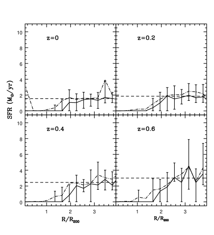
Figure 6: As in figure 5, but for a model in which $\alpha$ is constant .

We conclude that the hierarchical assembly of clusters in a $\Lambda$CDM cosmology can drive strong radial gradients in the star formation rates of cluster galaxies. Evolution in the number of star-forming galaxies at the centres of clusters at redshifts below 1 would indicate that galaxies are either more gas rich at high redshift or that processes that strip gas and quench star formation operate less efficiently in high redshift clusters.

6.2 Comparison with Data

Balogh et al (1998) have analyzed radial trends in the [OII] equivalent widths of galaxies in the CNOC1 sample. They find that the mean rest-frame equivalent width of the [OII]$\lambda$ 3727 emission line decreases by more than a factor of 10 from the outskirts of the clusters to the innermost regions. Even at distances of 1-2 virial radii from the cluster centres, galaxies have lower mean [OII] equivalent width than in the field. Ellingson et al (1999) have performed a principal component analysis of the CNOC1 spectra and also find strong gradients in the stellar populations of cluster galaxies.

In figures 7 and 8 we compare the star formation gradients as a function of projected radius obtained for the CNOC1 and simulated clusters. We have used the same star formation prescription as in figure 5 and have selected only galaxies with R-magnitudes brighter than -20.5. We also add a 1$\sigma$ error of 0.2 h^-2 M_⊙ yr^-1 to the star formation rates of the simulated galaxies. One consequence is that the differences seen in figures 5 and 6 are no longer observable and the two different star formation prescriptions give almost indistinguishable results at $z<0.6$. We scale the star formation rates of our cluster galaxies by dividing them by the median star formation rate of field galaxies in the low redshift sample. Finally, we randomly select the same number of galaxies in each radial bin as in the data.

The star formation rate distributions of cluster galaxies relative to the field look quite similar in the simulations and in the data. The median star formation rate is very close to zero near the cluster centre and rises to about one half the field value at $R_{proj}\sim R_{200}$. This is true in both the low– and high-redshift clusters. It should be noted that the trend in star formation rate as a function of projected clustercentric radius is much less abrupt than the trend as a function of physical radius from the cluster centre (Fig. 5). This means that it is important to include projection effects when carrying out detailed comparisons between simulations and data.

Figure 7: The star formation rates of galaxies with $M_{R}<-20.5$ are plotted as a function of scaled projected radius $R_{proj}/R_{200}$ for the CNOC1 sample. The star formation rates have been scaled by dividing by the median star formation rate of field galaxies of the same magnitude in the low redshift sample and adding 1 (so that negative star formation rates do not look pathological in the plot). The filled circles show the median star formation rate as a function of $R_{proj}$ and the error bars show the 25th to 75th percentiles of the distribution. The dotted line shows the median star formation rate of field galaxies with $M_{R}<-20.5$ at the same redshift.

Figure 8: The same as figure 7, except for the simulated clusters.

One striking difference between the simulations and the data is that the median star formation rate in the field appears to increase with redshift much more strongly in the data than in the model. This is apparent in figure 7, where the median star formation rate increases by a factor of $\sim 3$ over the redshift range considered, while there is very little increase apparent in figure 8. In figures 9 and 10, we plot the fraction of cluster galaxies with star formation rates greater than the median rate in the field as a function of projected clustercentric radius. At $z\sim 0.2$, the simulation results agree with the observations quite well. The fraction of galaxies with star formation greater than the field median increases from $\sim 0.1$ at the cluster centres to $\sim 0.3$ at $R_{proj}=R_{200}$. At $z\sim 0.4$, the fraction of galaxies in the CNOC1 clusters with star formation rates greater than the field median has decreased. This comes about because the star formation rates of galaxies in clusters do not appear to evolve significantly over this redshift interval (figure 7), but the median star formation rate in the field has gone up by more than a factor of two. We do not see the same effect in the simulations. When scaled to the field, cluster star formation rates evolve very little. At $z=0.8$, there is a hint that the number of strongly star-forming galaxies at the outskirts of the clusters has begun to increase.

We caution that the field samples in the CNOC1 survey are small, particularly at $z<0.3$. It will be interesting to see whether the strong evolution in the CNOC1 field sample is confirmed by the CNOC2 survey (Lin et al 1999).

Figure 9: The fraction of galaxies in CNOC1 clusters with $M_{R}<-20.5$ and star formation rate greater than the field median (at the same redshift) is plotted as a function of scaled projected radius $R_{proj}/R_{200}$. Circles show results for clusters at $0.18<z<0.3$ and squares are for clusters with $0.3<z<0.55$. Error bars are computed from jackknife estimation.

Figure 10: The same as figure 9 except for the simulated clusters. Circles are for clusters at $z=0.2$, squares for clusters at $z=0.4$ and triangles for clusters at $z=0.8$.

7 Colours and Mass-to-light Ratios

7.1 Colour Gradients

It has been known for some time that galaxies in the inner regions of clusters are redder than galaxies in the outer regions (Butcher & Oemler 1984; Millington & Peach 1990). Recently, large redshift surveys such as CNOC1 have reduced uncertainties in colour measurements due to the subtraction of background galaxies and have enabled the colour gradients of clusters to be studied in detail out to larger radii (Abraham et al 1996; Carlberg, Yee & Ellingson 1997).

In figures 11 and 12 we compare the rest-frame $B-V$ colours of cluster galaxies as a function of $R_{proj}/R_{200}$. Once again we have selected galaxies with rest-frame R-band magnitudes brighter than -20.5. We have added a 1$\sigma$ error of 0.07 mag in $B-V$ to the colours of the simulation galaxies in order to mimic the photometric uncertainties in the data. It is reassuring that our comparison of the colour gradients leads to exactly the same conclusion as the comparison of the star formation gradients. The colours of cluster galaxies in the simulation agree quite well with the data, but there is much stronger evolution in the colours of field galaxies in the CNOC1 survey. At $z=0.2$, field galaxies in the simulation are 0.1 mag too blue and at $z=0.4$ they are 0.1 mag too red. We note that the model colours do not include any correction for dust extinction.

Figure 11: The rest-frame $B-V$ colours of CNOC1 galaxies with $M_{R}<-20.5$ as a function of $R_{proj}/R_{200}$. Filled circles show the median colour as a function of $R_{proj}$ and error bars indicate the 25th to 75th percentiles of the distribution. The dotted line is the median colour of field galaxies at the same redshift.

Figure 12: As in figure 11, except for galaxies in the simulated clusters.

7.2 A comment on the Butcher-Oemler Effect

A major motivation for studying galaxy populations in clusters at intermediate redshifts has been the so-called Butcher-Oemler effect. Butcher & Oemler (1984) studied the fraction of bright galaxies $f_{B}$ contained in the inner regions of clusters that had rest-frame $B-V$ colours at least 0.2 mag bluer than the locus of the red elliptical galaxy population. They found a strong increase in $f_{B}$ from values of only a few percent in redshift zero clusters to $f_{B}\sim 0.25$ in clusters at $z=0.4$. This rapid evolution in the galaxy populations in clusters is puzzling, especially in light of other observational evidence indicating that the abundance of massive clusters has undergone only mild evolution since $z\sim 0.5$ (e.g. Bahcall, Fan & Cen 1997). Kauffmann (1995b) showed that a strong increase in $f_{B}$ over this redshift range is expected only in cosmologies where clusters assemble relatively late, such as a high-density ($\Omega_{matter}=1$) CDM cosmology with low normalization ($\sigma_{8}=0.4$), or a mixed dark matter (MDM) cosmology. In low-density CDM cosmologies, rather little evolution in $f_{B}$ was obtained out to $z=0.4$.

Figure 11 demonstrates that the Butcher-Oemler effect is observed in the CNOC1 cluster sample (see also Ellingson et al 2000; Yee et al, in preparation). Although the median colour of cluster galaxies differs very little between the high- and low-redshift samples, the 25th percentile of the colour distribution is considerably bluer for clusters with $0.3<z<0.55$ than it is for clusters with $0.18<z<0.3$. A similar effect is seen in the simulated clusters, but it is significantly weaker. It should be noted that the colour distribution of CNOC1 field galaxies has also shifted significantly bluewards over this redshift range.

As discussed previously, galaxies with large velocity differences from central cluster galaxies have been excluded from the cluster sample. Some fraction of the galaxies will nevertheless be interlopers from the field. We can study this in detail in our simulated cluster sample, where we have full position and velocity information for all galaxies, but we have selected cluster members using the same procedures as in the observations. In figure 13, we plot the fraction of galaxies that lie at physical distances larger than $R_{200}$ as a function of projected clustercentric distance. This fraction goes to 1 at $R_{proj}=R_{200}$. At the centres of clusters, the interloper fraction in the total sample is small ($\sim$ 10%). The fraction of red ($B-V>0.85$) cluster members that are interlopers is even smaller ( $\sim$ 3 %). However, more than 50% of galaxies with $B-V$ colours 0.2 magnitudes bluer than the locus of bulge-dominated galaxies are interlopers.

We conclude from this analysis that caution must be exercised in interpreting the physical origin of the Butcher-Oemler effect. At least part of the effect may be intrinsic to the field rather than to the cluster environment, and projection effects must be taken into account.

Figure 13: The fraction of simulated galaxies that lie at physical distances larger than $R_{200}$ from the cluster centre as a function of scaled projected radius $R_{proj}/R_{200}$. Galaxies are selected to have R-band magnitudes brighter than -20.5. The solid line shows results for all galaxies, the long-dashed line for galaxies with $B-V>0.85$ and the short-dashed line for galaxies with $B-V<0.65$.

7.3 The Colours of Bulge– and Disk–Dominated Galaxies as a Function of Clustercentric Radius

Early-type galaxies in nearby rich clusters follow a tight colour-magnitude relation (Bower, Lucey & Ellis 1992), Mg₂–$\sigma$ relation (Guzman et al 1992) and Fundamental Plane (eg. Jorgensen, Franx & Kjaergaard 1993). The small intrinsic scatter in these relations have been used as an argument that the early-type galaxies in these clusters formed at high redshift, or that their formation was synchronized (Bower, Lucey & Ellis 1992).

Kauffmann & Charlot (1998) have demonstrated that models in which early-type galaxies form by merging can also reproduce the observed scatter in the colour-magnitude relation of cluster ellipticals. One prediction of their models was that field ellipticals should form later than cluster ellipticals and should thus have younger stellar populations and exhibit greater scatter in colours and line indices.

There is some observational evidence in favour of younger ages for field ellipticals (Menanteau et al 1999; Schade et al 1999; Kodama, Bower & Bell 1999; Trager 1999), although some studies yield conflicting results (see for example Bernardi et al 1998 ; Kochanek et al 1999). Part of the reason for the discrepancy between different studies may lie in differing definitions of “field” versus “cluster”. This ambiguity may be overcome by studying trends in the colours of ellipticals as a function of distance from the cluster centre. Our model predictions for the colours of bulge-dominated (B) and disk-dominated (D) galaxies as a function of $R_{proj}/R_{200}$ are shown in figure 14. We have again selected galaxies with R-band magnitudes brighter than -20.5. In this plot, we have not added any artificial photometric errors, so the error bars represent the intrinsic 1$\sigma$ scatter in colour of the objects in each radial bin. We have also plotted the average colours of B and D galaxies in the CNOC1 clusters for comparison. The colours of both types of galaxies become bluer further from the cluster centre, but B galaxies are on average $\sim 0.1$ mag redder than D galaxies at all radii. The colour difference between the two classes appears to increase in high redshift clusters. This is also seen in the observations. Near the centres of clusters, B galaxies exhibit considerably smaller scatter in colour than D galaxies, but in the outer regions both types have similar scatter. Because the intrinsic scatter in colour predicted by our models is small compared with the photometric uncertainties of the CNOC1 data, we do not show the scatter in the observed colours in figure 14.

Figure 14: Average rest-frame $B-V$ colour as a function of projected clustercentric radius for B galaxies ($B/T>0.4$) and D ($B/T<0.2$) galaxies with R-band magnitudes brighter than -20.5 in the simulations. The error bars show the intrinsic 1$\sigma$ scatter in colour in each radial bin. The dashed lines in the right-hand panels are simply repeats of the solid lines in the left-hand panel, so that the reader is able to see the offset between the colours of the two classes. The triangles and squares show average colours of B and D galaxies in the CNOC1 clusters.

7.4 Colour as a Function of Cluster Mass

It is interesting to investigate whether the mean colours of galaxies depend on the mass of the cluster in which they are located. Naively, one would expect galaxies in more massive clusters to be older and hence redder, simply because galaxies form at higher redshifts if they are embedded in a more overdense region of the Universe (Bardeen et al 1986).

Our model predictions are shown in figure 15. We plot the mean rest-frame B-V colour of bulge-dominated ($B/T>0.4$) and disk-dominated ($B/T<0.2$) galaxies as a function of the mass of the halo in which they are located. We select only galaxies with $M_{R}<-20.5$ located less than $R_{200}$ from the cluster centre. There is a strong dependence of colour on halo mass for halos less massive than $5\times 10^{13}M_{\odot}$. This is because the galaxies in the sample undergo a transition from “central” galaxies that accrete gas from the surrounding halo and have ongoing star formation, to “satellite” galaxies that have been stripped of their hot gas halos and have no ongoing star formation. The precise halo mass at which this transition occurs thus will depend sensitively on the masses of the galaxies in the sample. For halos more massive than $5\times 10^{13}M_{\odot}$, the dependence of galaxy colour on cluster mass is relatively weak.

We note that the colours of disk-dominated galaxies as a function of cluster mass may place important constraints on gas removal in galaxies by ram-pressure stripping because the effect depends strongly on the mass of the cluster.

Figure 15: Average rest-frame $B-V$ colour of bulge-dominated (B) (solid line) and disk-dominated (D) (dashed line) galaxies as a function of the mass of the halo in which they are located. Error bars show the $1-\sigma$ scatter in the intrinsic colour of the galaxy. Only galaxies with $M_{R}<-20.5$ that lie inside $R_{200}$ are included in the samples.

7.5 Mass-to-light Ratios

The evolution of the stellar mass-to-light ratios of early-type galaxies provide a more sensitive test of the ages of their stellar populations than their colours, mainly because the mean luminosity evolution of an old stellar population is large compared to its mean colour evolution. Van Dokkum et al (1998b) find slow luminosity evolution of early-type galaxies to $z=0.8$ and show that if one were comparing similar kinds of objects at all redshifts, one would infer that the majority of their stars were formed at $z>1.7$ for a Salpeter IMF and a cosmology with $\Omega=0.3$ and $\Lambda=0.7$. In figure 16, we compare the evolution of the B-band M/L ratios of bulge-dominated galaxies in our simulated clusters with data from Van Dokkum et al (1998b) plotted for a $\Lambda$CDM cosmology. We have selected galaxies with rest-frame B-band magnitudes less than than -21.5 (corresponding to galaxies with $I<22.1$ in the observed sample) and $B/T>0.4$ that lie at distances less than $R_{200}$ from the cluster centre. As can be seen, the agreement is good.

Figure 16: The evolution of the B-band mass-to-light ratio of bulge-dominated ($B/T>0.4$) galaxies in clusters. The solid line shows the shift in the mean M/L in the simulated galaxies. The points with error bars are taken from Van Dokkum et al. (1998b)

8 Morphologies and Morphology Gradients

8.1 Evolution of Morphology Gradients

In nearby clusters the morphologies of galaxies are correlated with distance from the cluster centre. Whitmore, Gilmore & Jones (1993) have studied the relation between morphology and clustercentric radius in Dressler’s sample of 6000 galaxies in 55 nearby clusters. They find that if they normalize the clustercentric distances by a characteristic cluster radius $R_{c}^{opt}$, corresponding to the radius within which the density of bright galaxies has some fixed value, the morphology-radius relation is “universal” and does not vary with cluster richness, velocity dispersion or X-ray luminosity. The fraction of spiral and irregular galaxies increases from near zero at the cluster center to $\sim 0.6$ at the outskirts of the cluster.

Trends in morphology have also been studied in a number of high redshift clusters ( e.g. Abraham et al 1996; Dressler et al 1997 ; Balogh et al 1998; Couch et al 1998; Van Dokkum et al 2000).

An increase in the fraction of early-type galaxies towards the centres of clusters is observed in all cases, but the detailed evolution of the morphology-radius relation to high redshift remains a subject of considerable controversy. Dressler et al. (1997) claim that the fraction of elliptical galaxies in rich clusters remains constant with redshift, but the fraction of S0 galaxies at $z\sim 0.4$ is a factor 2-3 times smaller than at present with a proportional increase in the numbers of spirals. This has recently been confirmed by a separate study by Fasano et al (2000). Van Dokkum et al (2000) dispense with the distiction between elliptical and S0, and study the evolution of the fraction of early-type galaxies in rich clusters. They claim that there is a clear trend for high-redshift clusters to have lower early-type fractions than low-redshift clusters. Within a fixed physical radius of 300 $h^{-1}$ kpc, the early-type fraction appears to decline by a factor of two from $\sim 0.8$ at $z=0$ to $\sim 0.4$ at $z=0.8$.

One major difficulty in comparing our morphology gradients with observational data is that it is not clear whether the classification of galaxies according to $B/T$ corresponds in any simple way to “by eye” classifications according to Hubble type. In this section, we compare our $z=0.2$ morphology-radius relation with the CNOC1 sample of cluster galaxies for which classifications according to $B/T$ are available for $\sim$75% of the sample (the galaxies that are exluded show no correlation with redshift, emission line properties or colour (Balogh et al 1998)). We select only galaxies with R-band absolute magnitudes brighter than -20.5 in both the data and in the simulations. Cluster membership is defined as described previously.

The fractions of galaxies in each class as a function of projected clustercentric radius are shown in figures 17 and 18. The gradient of bulge-dominated galaxies agrees remarkably well with the observations. It exhibits a steep drop from the cluster centre out to a radius of $\sim 0.5R_{200}$ and then flattens in the outer regions of the cluster. The fractions of disk-dominated and intermediate galaxies do not agree as well. There are too many disk-dominated galaxies in the cluster and not enough intermediate systems, suggesting that additional processes may lead to bulge formation and/or disk destruction in the cluster.

Figure 17: The fraction of bulge-dominated (solid squares), disk-dominated (open squares) and intermediate-type (open triangles) galaxies is plotted as a function of scaled projected radius for the CNOC1 clusters. The error bars present the Poisson errors. The symbols on the right-hand side of the plot indicate the fractions in the field.

Figure 18: As in figure 17, except for the simulated clusters. The boundaries between the morphological classes were chosen so that the field fractions match those in figure 17.

The morphology-radius relation in the simulation does not evolve noticeably with redshift. This is shown again in fig 19, where we plot the fraction of bulge-dominated ($B/T>0.4$) galaxies inside $R_{200}$ for each cluster as a function of its redshift. There is a fairly large cluster-to-cluster scatter, but no evidence of a decline in the fraction of bulge-dominated galaxies at high redshifts. However, as we show in section 8.2, the fraction of bulge-dominated galaxies depends on cluster mass, so this result will be sensitive to how clusters are selected observationally.

Figure 19: The fraction of galaxies inside $R_{200}$ with $B/T>0.4$ is plotted against redshift for each cluster in the sample.

8.2 Distribution of morphologies as a function of cluster mass

In figure 20 we show how the fractions of bulge-dominated (B) and disk-dominated (D) galaxies vary as a function of the mass of the cluster. We have selected galaxies with $M_{R}<-20.5$ located less than $R_{200}$ from the cluster centre.

The B fraction shows a pronounced peak for clusters $\sim 3\times 10^{14}M_{\odot}$ and then declines for masses larger than this. The D fractions mirror this trend, showing a significant increase for the most massive clusters.

Whitmore, Gilmore & Jones (1993), find no dependence of galaxy morphology on the X-ray luminosity or the velocity dispersion of the clusters in their sample. Figure 20 indicates that the dependence of morphology on cluster mass is stronger at high redshift than at low redshift, so it would be very interesting to repeat their analysis for a sample of higher redshift clusters. Fasano et al (2000) find a strong dependence of the relative numbers of elliptical and S0 galaxies on cluster type. In particular, clusters in which the population of ellipticals is strongly concentrated have fewer S0 galaxies.

Figure 20: The solid line shows the fraction of galaxies with $M_{R}<-20.5$ and $B/T>0.4$ located inside $R_{200}$ as a function of the virial mass of the cluster. The dashed line is for galaxies with $B/T<0.2$. Error bars show the $1-\sigma$ scatter between different clusters of the same mass in the simulation.

8.3 The relation between morphology and star formation rate

In previous sections we have compared the star formation rate and morphology gradients in our simulated clusters with the CNOC1 data and have found reasonably good agreement. Here we compare the star formation rate distributions of disk-dominated (D) and bulge-dominated (B) galaxies in clusters. Figures 21 and 22 compare the star formation rate distributions of galaxies in these these two classes at two different redshifts. Unlike bulge-dominated galaxies, the SFR distribution of disk galaxies exhibit a pronouced tail of higher star formation rate systems. Moreover, the fraction of disk galaxies in the tail appears to increase to higher redshift. This increase is seen in both the simulated clusters and in the CNOC1 clusters, but appears somewhat stronger in the latter.

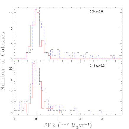
Figure 21: The solid line shows the star formation rate distribution of bulge-dominated galaxies in the CNOC1 clusters, while the dashed line shows the star formation rate distribution of disk-dominated systems. We have selected galaxies with R-band magnitudes less than -20.5.

Figure 22: As in figure 21, except for the simulated clusters.

9 The kinematics of cluster galaxies

The existence of combined information on the spatial and kinematic distributions of cluster galaxies as a function of colour and morphological type provides fundamental constraints on how clusters were formed and on how their galaxy populations were accreted (e.g. Dickens & Moss 1976; Colless & Dunn 1996; Mohr et al. 1996; Carlberg et al 1997; Biviano et al 1997; Fisher et al 1998; De Theije & Katgert 1999). The line-of-sight velocity dispersions of star-forming galaxies are $\sim 20-40\%$ larger than the velocity dispersions of non-star forming galaxies. This result suggests that the star-forming galaxies are on fairly radial, ‘first-approach’ orbits towards the central regions of their clusters, and are not yet in equilibrium with the population of non-star forming galaxies. Figure 23 shows the differential velocity dispersion profiles for red/blue and bulge-dominated/disk-dominated galaxies in our simulated clusters at two different redshifts. Velocities are in units of $V_{200}$, the cluster circular velocity at $R_{200}$.

As discussed previously, blue galaxies have just been accreted by the cluster. They are less bound and their velocity dispersions in the central regions of clusters are $\sim 30\%$ larger than those of red galaxies. Figure 23 indicates that there is rather little change in the velocity profiles of galaxies between low and high redshift clusters if we split our sample at the median colour at each redshift.

In contrast, there is almost no difference in the differential velocity dispersion profiles of bulge-dominated and disk-dominated cluster galaxies. In our models, the morphological evolution of cluster galaxies and their star formation histories are decoupled. We have shown that clusters contain a substantial population of red disk-dominated galaxies that were accreted more than $\sim 1-2$ Gyr ago and are thus in dynamical equilibrium within the cluster. This compensates for the larger velocities of the recently-accreted, star-forming disk galaxies.

These results are in good agreement the CNOC1 data. Figure 24 shows the differential velocity dispersions of CNOC1 cluster galaxies: the red and blue subsamples have clearly distinct profiles in the central regions, whereas the bulge-dominated and disk-dominated galaxies have indistinguishable profiles. The lines show the model predictions for model galaxies with the same selection criteria as in the data.

In the simulations, red and blue galaxies do not show any difference in their orbital parameters: Figure 25 shows the profile of the velocity anisotropy parameter $\beta(r)=1-\langle v_{t}^{2}\rangle/2\langle v_{r}^{2}\rangle$, where $v_{r}$ and $v_{t}$ are the radial and tangential components of the galaxy velocities respectively. Both red and blue galaxies have $\beta(r)$ similar to that of the dark matter and smaller than 0.5. This result indicates that the velocity distribution is close to isotropic as also inferred for the CNOC1 clusters by Van der Marel et al. (1999). Note that Figure 25 shows the profile averaged over all the massive clusters in our simulation box. Individual clusters may exhibit larger velocity anisotropies; however, we never find any substantial differences between blue and red galaxies. Splitting the galaxy sample according to the star formation rate does not change our conclusion.

Figure 23: Evolution of the differential velocity dispersion profiles for clusters with $M_{200}>10^{14}M_{\odot}$. Solid lines are the dark matter profiles; dashed (dotted) lines are the profiles of red (blue) galaxies or bulge-dominated ( disk-dominated) galaxies. In the left panels, the galaxy sample is separated according to the median rest-frame colour $B-V$ at each redshift; in the right panels, B (D) type galaxies have bulge-to-total luminosity ratio $B/T>0.4$ ($B/T<0.2$). The galaxy sample only includes galaxies brighter than $M_{R}=-20.5$. Note that both red and bulge-dominated galaxies track the differential velocity dispersion profiles of the dark matter component reasonably well both at low and high redshifts.

Figure 24: Differential velocity dispersion profiles of galaxies brighter than $M_{R}=-20.5$ in the CNOC1 clusters. The top panel shows the profiles of blue (open squares) and red (filled squares) galaxies; the rest-frame colour threshold is $B-V=0.85$. The dashed and the solid lines show the corresponding profiles of the blue and red galaxies in the simulated clusters. The bottom panel shows the profile of D galaxies (open squares) and B galaxies (filled squares) galaxies in the data. The dashed and the solid lines show the profiles of the model D and B galaxies respectively. In both panels, simulated clusters are at $z=0.2$, and error bars on the data are the standard deviations computed with the bootstrap method.

Figure 25: Evolution of the average profiles of the velocity anisotropy parameter $\beta(r)$ in clusters with $M_{200}>10^{14}M_{\odot}$. The thick lines are as for Figure 23. The thin lines indicate the $1-\sigma$ bootstrap fluctuations. For clarity we omitted the profiles where poor statistics yields a 1-$\sigma$ bootstrap range larger than 2.8.

10 Summary and Discussion

In this paper, we demonstrate how combining semi-analytic modelling of galaxies with N-body simulations of cluster formation allows us to study spatial variations in the colours, star formation rates and morphologies of cluster galaxies and their evolution with redshift. We have shown that gradients in galaxy properties arise naturally in hierarchical models, because mixing is incomplete during cluster assembly. The positions of galaxies within the cluster are correlated with the epoch at which they were accreted. As a result, galaxies in the cores of clusters have lower star formation rates, redder colours and larger bulge-to-disk ratios than galaxies in the outer regions. We have also demonstrated that star-forming cluster galaxies have larger velocity dispersions than non-starforming galaxies. Our models predict that the mean colours and star formation rates of cluster galaxies become equal to the field values at distances of $\sim 2-3R_{200}$ from the cluster centre.

We have compared our derived gradients with recent observational data from the CNOC1 cluster survey. Our star formation rate and colour gradients agree reasonably well with the data. In agreement with Balogh, Navarro & Morris (2000), we find that the CNOC1 results are consistent with a picture in which star formation is gradually terminated over a period of 1-2 Gyr after galaxies fall into the cluster. We also study the velocity dispersion profiles of cluster galaxies in our simulations as a function of colour and find that they match the data.

Our models are also reasonably successful in explaining the observed trends in galaxy morphology as a function of clustercentric radius. For simplicity we have assumed that a galaxy’s morphology is determined solely by its history of major mergers. A major merger leads to the formation of a bulge and any gas that cools thereafter forms a new disk. We have shown that this model works very well for bulge-dominated galaxies, but is less successful in explaining the observed fractions of galaxies with intermediate and low bulge-to-disk ratios. In order to bring our results into agreement with observations, some additional process must either destroy existing disks or form new bulges in cluster galaxies. This suggests that ram-pressure stripping or galaxy harassment may affect the morphologies of galaxies, but have little effect on their star formation rates.

We have also studied how star-formation rates of cluster galaxies vary as a function of bulge-to-disk ratio and as a function of redshift in the CNOC1 and simulated clusters. The star formation rate distributions of bulge-dominated and disk-dominated cluster galaxies are peaked near zero, but disk galaxies exhibit a tail of higher star formation rate systems. The fraction of the population in this tail appears to increase to higher redshift. The star formation rates of bulge-dominated galaxies evolve much more weakly with redshift.

In our models, the evolution of the star formation rates and the morphologies of cluster galaxies are largely decoupled. We predict that the colours of cluster galaxies are largely independent of the mass of the cluster, but that there is a strong dependence of morphology on cluster mass. In particular, more massive clusters are predicted to contain a smaller fraction of bulge-dominated galaxies formed by major mergers.

We find that the major disagreement between the simulations and the CNOC1 data occurs not for cluster galaxies, but for field galaxies. Bright CNOC1 field galaxies evolve dramatically in star formation rate and in colour over the redshift range $0.18<z<0.55$. This is not seen in the simulations. We have argued that this rapid evolution in star formation rate in the field may also be manifested as a strong apparent increase in the number of blue galaxies in clusters at high redshift, because a large fraction of the blue cluster members in our simulation are in fact interlopers from the field. We have chosen not to delve further into the issue of field galaxy evolution in this paper, because the CNOC1 field sample is rather small and is not selected in a completely unbiased way due to the fact that the fields always contain a rich cluster. It is therefore not the ideal sample for a detailed comparison between theory and observations.

Finally, our analysis demonstrates how important it is for simulation data to be analyzed the same way as the observations. The star formation and morphology gradients plotted as a function of projected radius can differ substantially from the true physical gradients. Although interlopers from the field may be a small fraction of the total cluster sample, they may be a more significant component of the blue population, which is intrinsically rare in the centres of clusters.

Acknowledgments
The simulations in this paper were carried out using codes kindly made available by the Virgo Consortium. We especially thank Jörg Colberg and Adrian Jenkins for help in carrying them out. GK thanks Pieter van Dokkum and Richard Ellis for helpful discussions. We would also like to thank members of the CNOC1 team for allowing us to use their data in advance of full publication. MLB gratefully acknowledges support from a PPARC rolling grant for extragalactic astronomy and cosmology at the University of Durham.

References

- [1] Abadi, M.G., Moore, B. & Bower, R.G., 1999, MNRAS, 308, 947
- [2] Abraham, R.G., Smecker-Hane, T.A., Hutchings, J.B., Carlberg, R.G., Yee, H.K.C., Ellingson, E., Morris, S., Oke, J.B. & Rigler, M., 1996, ApJ, 471, 694
- [3] Bahcall, N., Fan, X. & Cen, R., 1997, ApJ, 485, L53
- [4] Balogh, M.L., Morris, S.L., Yee, H.K.C., Carlberg, R.G. & Ellingson, E., 1997, ApJ, 488, 75
- [5] Balogh, M.L., Schade, D., Morris, S.L., Yee, H.K.C., Carlberg, R.G. & Ellingson, E., 1998, ApJ, 504, 75
- [6] Balogh, M.L., Morris, S.L., Yee, H.K.C., Carlberg, R.G. & Ellingson, E., 1999, ApJ, 527, 54
- [7] Balogh, M.L., Navarro, J.F. & Morris, S.L., 2000, astro-ph/0004078
- [8] Barbaro & Poggianti, 1997, A&A, 324, 490
- [9] Bardeen, J.M., Bond, J.R., Kaiser, N. & Szalay, N., 1986, ApJ, 304, 15
- [10] Benson, A.J., Cole, S., Frenk, C.S., Baugh, C.M. & Lacey, C., 2000, MNRAS, 311, 793
- [11] Bernardi, M., Renzini, A., Da Costa, L., Wegner, G., Alonso, M.V., Pellegrini, P.S., Rite, C. & Willmer, C.N.A., 1989, ApJ, 508, 143
- [12] Biviano, A., Katgert, P., Mazure, A., Moles, M., Den Hartog, R., Perea, J. &Focardi, P., 1997, A&A, 321, 84
- [13] Bond, J.R., Cole, S., Efstathiou, G. & Kaiser, N., 1991, ApJ, 379, 440
- [14] Bower, R.G., 1991, MNRAS, 248, 332
- [15] Bower, R.G., Lucey, J.R. & Ellis, R.S., 1992, MNRAS, 254, 601
- [16] Butcher, H. & Oemler, A., 1978, ApJ, 219, 18
- [17] Butcher, H. & Oemler, A., 1984, ApJ, 285, 426
- [18] Byrd, G. & Valtonen, M., 1990, ApJ, 350, 89
- [19] Carlberg, R.G. Yee, H.K.C., Ellinson, E., Abraham, R.G., Gravel, P., Morris, S. & Pritchet, C.J., 1996, ApJ, 462, 32
- [20] Carlberg, R.G., Yee, H.K.C., Ellingson, E., Morris, S.L., Abraham, R., Gravel, P., Pritchet, C.J., Smecker-Hane, T., Hartwick, F.D.A. et al, 1997, ApJ, 476, L7
- [21] Carlberg, R.G., Yee, H.K.C. & Ellingson, E., 1997, ApJ, 478, 462
- [22] Coleman, G. D., Wu, C. & Weedman, D. W. 1980, ApJS, 43, 393
- [23] Colless, M. & Dunn, A.M., 1996, ApJ, 458, 435
- [24] Couch, W.J., Ellis, R.S., Sharples, R.M. & Smail, I., 1994, ApJ, 430, 121
- [25] Couch, W.J., Barger, A.J., Smail, I., Ellis, R.S. & Sharples, R.M., 1998, ApJ, 497, 188
- [26] De Propris, R., Stanford, S.A., Eisenhardt, P.A., Dickinson, M. & Elston, R., 1999, AJ, 118, 719
- [27] De Theije, P.A.M. & Katgert, P., 1999, A&A, 341, 371
- [28] Diaferio, A., Kauffmann, G., Colberg, J.G. & White, S.D.M., 1999, MNRAS, 307, 537
- [29] Dickens, R.J. & Moss, C., 1976, MNRAS, 174, 47
- [30] Dressler. A., Oemler, A., Couch, W.J., Smail, I., Ellis, R.S., Barger, A., Butcher, H., Poggianti, B.M. & Sharples, R.M., 1997, ApJ, 490, 577
- [31] Dressler, A., Smail, I., Poggianti, B.M., Butcher, H., Couch, W.J., Ellis, R.S. & Oemler, A., 1999, ApJS, 122,51
- [32] Eke, V.R., Navarro, J.F. & Frenk, C.S., 1998, ApJ, 503, 569
- [33] Ellingson, E., Lin, H., Yee, H.K.C. & Carlberg, R.G., 1999, astro-ph/9909074
- [34] Evrard, A.E., 1990, ApJ, 363, 349
- [35] Evrard, A.E., Silk, J. & Szalay, A.S., 1990, ApJ, 365, 13
- [36] Farouki, R. & Shapiro, S.L., 1980, ApK, 241,928
- [37] Fasano, G., Poggianti, B.M., Couch, W.J., Bettoni, D., Kjaergaard, P. & Moles, M.,2000, astro-ph/0005171
- [38] Fisher, D., Fabricant, D., Franx, M. & van Dokkum, P.G., 1998, ApJ, 498, 195
- [39] Fukugita, M., Shimasaku, K. & Ichikawa, T., 1995, PASP, 107, 945
- [40] Guzman, R., Lucey, J.R., Carter, D. & Terlevich, R.J., 1992, MNRAS, 257, 287
- [41] Hashimoto, Y., Oemler, A., Lin, H. & Tucker, D.L., 1998, ApJ, 499, 589
- [42] Hernquist, L., 1990, ApJ, 356, 359
- [43] Jorgensen, I., Franx, M. & Kjaergaard, P., 1993, ApJ, 411, 34
- [44] Kauffmann, G., 1995a, MNRAS, 281, 475
- [45] Kauffmann, G., 1995b, MNRAS, 281, 487
- [46] Kauffmann, G., Nusser, A. & Steinmetz, M., 1997, MNRAS, 286, 795
- [47] Kauffmann, G. & Charlot, S., 1998, MNRAS, 294, 705
- [48] Kauffmann, G., Colberg, J.G., Diaferio, A. & White, S.D.M., 1999a, MNRAS, 303, 188 (KCDW)
- [49] Kauffmann, G., Colberg, J.G., Diaferio, A. & White, S.D.M., 1999b, MNRAS, 307, 529
- [50] Kauffmann, G. & Haehnelt, M., 2000, MNRAS, 311, 576
- [51] Kennicutt, R.C., Tamblyn, R. & Congdon, C.E., 1994, ApJ, 435, 22
- [52] Kennicutt, R.C., 1998, ApJ, 498, 541
- [53] Kennicutt, R.C., 1998, ARAA, 36, 189
- [54] Klypin, A., Gottloeber, S., Kravtsov, A.V. & Khoklhov, A.M., 1999, ApJ, 516, 530
- [55] Kochanek, C.S., Falco, E.E., Impey, C.D., Lehar, J., Mcleod, B.A., Rix, H.-W., Keeton, C.R., Munoz, J.A. & Peng, C.Y., 1999, astro-ph/9909018
- [56] Kodama, T., Bower, R.G. & Bell, E., 1999, MNRAS 306, 561
- [57] Kolatt, T.S., Bullock, J.S., Somerville, R.S., Sigad, Y. Jonsson, P., Kravtsov, A.V., Klypin, A.A., Primack, J.R. et al., 1999, ApJ, 523, L109
- [58] Lavery, R.J. & Henry, P.J., 1988, ApJ, 330, 596
- [59] Lin, H., Yee, H.K.C., Carlberg, R.G., Morris, S.L., Sawicki, M., Patton, D.R., Wirth, G. & Shepherd, C.W., 1999, ApJ, 518, 533
- [60] Lubin, L.M., Postman, M., Oke, J.B., Ratnatunga, K.U., Gunn, J.E., Hoessel, J.G. & Schneider, D.P., 1998, AJ, 116, 584
- [61] Menanteau, F., Ellis, R.S., Abraham, R.G., Barger, A.J. & Cowie, L.L., 1999, MNRAS, 309, 208
- [62] Millington, S.J.C. & Peach, J.V., 1990, MNRAS, 242, 112
- [63] Mohr, J., Geller, M.J., Fabricant, D.G., Wegner, G., Thostensen, J. & Richstone, D.O., 1996, ApJ, 470, 724
- [64] Moore, B., Katz, N., Lake, G., dressler, A. & Oemler, A., 1996, Nature, 379, 613
- [65] Navarro, J.F., Frenk, C.S. & White, S.D.M., 1995, MNRAS, 275, 56
- [66] Oemler, A., Dressler, A. & Butcher, H.D., 1997, ApJ, 474, 561
- [67] Patton, D. R., Pritchet, C. J., Yee, H. K. C., Ellingson, E., & Carlberg, R. G. 1997, ApJ, 475, 29
- [68] Poggianti, B.M., Smail, I., Dressler, A., Couch, W.J., Barger, A.J., Butcher, H., Ellis, R.S. & Oemler, A., 1999, ApJ, 518, 576
- [69] Schade, D., Lilly, S. J., Le Fèvre, O., Hammer, F. & Crampton, D. 1996a, ApJ, 464, 79
- [70] Schade, D., Carlberg, R. G., Yee, H. K. C., López–Cruz, O., & Ellingson, E. 1996b, ApJ, 464, L63
- [71] Schade, D., Lilly, S.J., Crampton, D., Ellis, R.S., Le Fevre, O., Hammer, F., Brinchmann, J., Abraham, R. et al., 1999, ApJ, 52, 31
- [72] Schmalzing, J. & Diaferio, A., 2000, MNRAS, 312, 638
- [73] Seljak, U., 2000, astro-ph/0001493
- [74] Sheth, R. & Diaferio, A., 2000, MNRAS, submitted
- [75] Somerville, R.S., Primack, J.R. & Faber, S.M., 1998, astro-ph/9806228
- [76] Springel, V., White, S.D.M., Tormen, G. & Kauffmann, G., 2000, MNRAS, submitted
- [77] Stanford, S.A., Eisenhardt, P.A. & Dickinson, M.E., 1998, ApJ, 492, 461
- [78] Tormen, G., Diaferio, A. & Syer, D., 1998, MNRAS, 299, 728
- [79] van den Bosch, F.C., Lewis, G.F., Lake, G. & Stadel, J., 1999, ApJ, 515, 50
- [80] van der Marel, R.P., Magorrian, J., Carlberg, R.G., Yee, H.K.C. & Ellingson, E., 1999, astro-ph/9910494
- [81] van Dokkum, P.G., Franx, M., Kelson, D.D., Illingworth, G.D., Fisher, D. & Fabricant, D., 1998, ApJ, 500, 714
- [82] van Dokkum, P.G., Franx, M., Kelson, D.D. & Illingworth, G.D., 1998b, ApJ, 504, 17
- [83] van Dokkum, P.G., Franx, M., Fabricant, D., Illingworth, G.D. & Kelson, D., 2000, astro-ph/0002507
- [84] Whitmore, B.C., Gilmore, D.M. & Jones, C., 1993, ApJ, 407, 489
- [85] Yee, H.K.C., Ellingson, E. & Carlberg, R.G., 1996, ApJS, 102, 269
- [86]