A New Analysis Method for Reconstructing the Arrival Direction of TeV Gamma-rays Using a Single Imaging Atmospheric Cherenkov Telescope

Abstract

We present a method of atmospheric Cherenkov imaging which reconstructs the unique arrival direction of TeV gamma rays using a single telescope. The method is derived empirically and utilizes several features of gamma-ray induced air showers which determine, to a precision of $0.12^{\circ}$, the arrival direction of photons, on an event-by-event basis. Data from the Whipple Observatory’s 10 m gamma-ray telescope is utilized to test selection methods based on source location. The results compare these selection methods with traditional techniques and three different camera fields of view. The method will be discussed in the context of a search for a gamma-ray signal from a point source located anywhere within the field of view and from regions of extended emission.

1 Introduction

The Whipple Collaboration operates a 10 m optical reflector for gamma-ray astronomy at the Fred Lawrence Whipple Observatory on Mt. Hopkins (elevation 2320 m) in southern Arizona. The reflector was originally constructed in 1968 weekes72 and numerous modifications have been made to improve the sensitivity and performance of the system. A camera consisting of photomultiplier tubes (PMTs) mounted in the focal plane of the reflector, detects the Cherenkov radiation produced by gamma-ray and cosmic-ray air showers from which an image of the Cherenkov light can be reconstructed. The camera is triggered when any two PMT signals are above a threshold within a short time coincidence.

In the past decade the camera has undergone significant expansion from a field of view (FOV) of $3.0^{\circ}$ in 1989 to a FOV of $4.8^{\circ}$ in 1999. From 1989 to 1996 the camera consisted of 109 PMTs, each viewing a circular field of $0.259^{\circ}$ diameter, yielding a total FOV of $3.0^{\circ}$. The trigger condition required any two of the inner 91 PMT signals to be above a threshold within a 15 ns time coincidence. During the spring of 1997 the camera was expanded to 151 PMTs yielding a total FOV of $3.5^{\circ}$. The trigger condition required any two of the inner 91 PMT signals ($3.0^{\circ}$ triggering FOV) to be above a threshold with a coincidence resolving time of 15 ns. From 1997 to 1999 the camera was further expanded to 331 PMTs yielding a total FOV of $4.8^{\circ}$. The trigger was expanded to include all 331 PMT signals and the time coincidence was shortened to 10 ns due to the introduction of constant fraction discriminators. The layout of each camera is depicted in Figure 1. A full description of the reflector, which has not changed since its original construction, can be found in cawley90 .

Primary cosmic rays and gamma rays entering the atmosphere initiate showers of secondary particles which propagate down towards the ground. The trajectory of the shower continues along the path of the primary particle. If the optical reflector lies within the 300 m diameter Cherenkov light pool, it forms an image in the PMT camera. The appearance of this image depends upon a number of factors. The nature and energy of the incident particle, the arrival direction and the point of impact of the particle trajectory on the ground, all determine the initial shape and orientation of the image. This image is modified by the point spread function of the telescope, the addition of instrumental noise in the PMTs and subsequent electronics, the presence of bright stellar images in certain PMTs and by spurious signals from charged cosmic rays physically passing through the tubes. Monte Carlo studies have shown that gamma-ray induced showers give rise to more compact images than background hadronic showers and are preferentially oriented towards the source position in the image plane hillas85 . By making use of these differences, a gamma-ray signal can be extracted from the large background of hadronic showers and a gamma-ray map over the FOV can be obtained. The method of extracting a gamma-ray signal from the hadronic background can be found in fegan94 . The technique of obtaining a gamma-ray map of the FOV, by reconstructing the unique arrival direction of very high energy photons, is the topic of this paper.

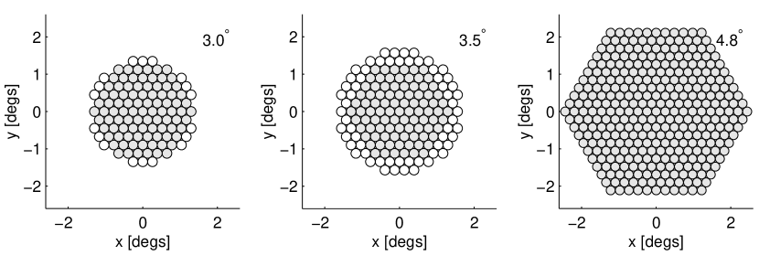
Figure 1: The PMT camera utilized by the Whipple Observatory’s 10 m gamma-ray telescope has undergone several upgrades over the past decade. Each camera is comprised of PMTs of the same model and size but with increasing FOV. The gray pixels depict the PMTs included in the trigger.

Data from the Whipple Observatory’s 10 m high energy gamma-ray telescope, will be used to demonstrate methods of the reconstruction of the arrival direction of gamma-ray induced showers. These methods may be applied a) to a search for point sources located anywhere within the camera’s FOV, for example searches for counterparts to EGRET unidentified sources, gamma-ray bursts, described in connaughton98 , or sky surveys and b) analysis of extended sources of TeV gamma-rays such as supernova remnants, described in buckley98 and Galactic plane emission described in lebohec2000 .

2 Shower Image Processing and Characterization

Prior to analysis of the recorded images, two calibration operations must be performed: the subtraction of the pedestal analog-digital conversion (ADC) values and the normalization of the PMT gains, a process known as flat-fielding.

The pedestal of an ADC is the finite value which it outputs for zero input. This is usually set at 20 digital counts so that small negative fluctuations on the signal line, due to night sky noise variations, will not generate negative values in the ADC. The pedestal for each PMT is determined by artificially triggering the camera, thereby capturing ADC values in the absence of genuine input signals. The PMT pedestal and pedestal variance are calculated from the mean and variance of the pulse-height spectrum (PHS) generated from these injected events.

The relative PMT gains are determined by recording a thousand images using a fast Optitron Nitrogen Arc Lamp illuminating the focal plane through a diffuser. These nitrogen pulser images are used to determine the relative gains by comparing the relative mean signals seen by each PMT.

Fluctuations in the image usually arise from electronic noise and night-sky background variations. To reject these distortions a PMT is considered to be part of the image if it either has a signal above a certain threshold or is beside such a PMT and has a signal above a lower threshold. These two thresholds are defined as the picture and boundary thresholds, respectively. The picture threshold is the multiple of the root mean square (RMS) pedestal deviation which a PMTs signal must exceed to be considered part of the picture. The boundary threshold is the multiple of the RMS pedestal deviation which PMTs adjacent to the picture must exceed to be part of the boundary. The picture and boundary PMTs together make up the image; all others are zeroed. This image cleaning procedure is depicted in Figure 2. These thresholds were optimized using data taken on the Crab Nebula yielding picture threshold: 4.25, and boundary threshold: 2.25.

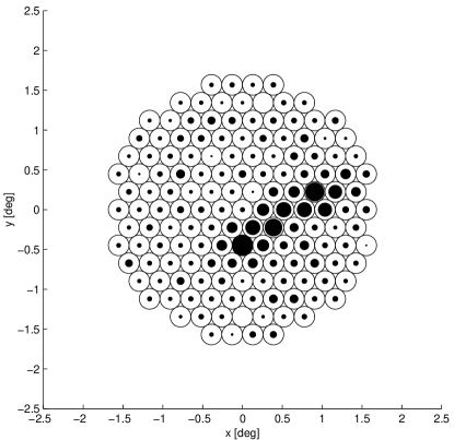
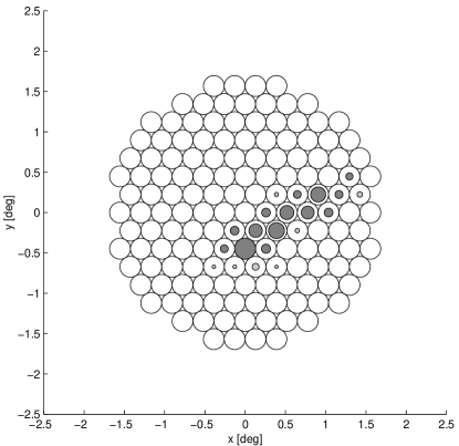
Figure 2: (Left) Example of an image prior to the processing procedure given in the text. Diameter of each filled circle is proportional to the ADC signal for that PMT. (Right) The same image after pedestal subtraction, application of picture (dark gray filled circles) and boundary (light gray filled circles) thresholds and gain normalization.

For the results reported in this paper, the data are obtained in an ON/OFF mode where the source position is tracked for 28 minutes (ON), followed by a 28 minute observation of a background region (OFF) covering the same path in elevation and azimuth. In an ON/OFF observation mode, differences in sky brightness between ON and OFF sky regions could introduce biases. These biases can severely affect the selection of pixels accredited to the boundary region and hence distort the Cherenkov image. For example, if the ON region is brighter than the OFF region, bias may arise as follows. Consider tubes which have a combination of small amounts of genuine signal coupled with some noise (e.g. boundary tubes). If the noise level is low, the boundary threshold is low and most of these tubes will pass the threshold test and be included as part of the image. However, if the noise level is high then the boundary threshold will also be high and the probability increases that a negative noise fluctuation will cancel the genuine signal component resulting in the tube being set to zero during image cleaning. Thus, the degree to which boundary tubes are set to zero depend on the noise level in the tubes. As a consequence a bright sky region will result in more boundary tubes being set to zero, making the image appear narrower and more gamma-ray like.

A software technique was developed to correct for the biases introduced by the differing sky brightness cawley93 . This technique, known as software padding works by adding software noise into the events for the darker sky region. Let $P_{\rm on}(P_{\rm off}),\sigma_{\rm on}(\sigma_{\rm off})$ be the ON(OFF) pedestal and pedestal deviation values for a particular pixel and $C_{\rm on}(C_{\rm off}),\sigma_{C_{\rm on}}(\sigma_{C_{\rm off}})$ be the component due to the Cherenkov signal and corresponding fluctuation. The total ON signal is

$${\rm ON}=P_{\rm on}+\sigma_{\rm on}Gauss(0:1)+C_{\rm on}+\sigma_{C_{\rm on}}Gauss(0:1),$$ (1)

where $Gauss(0:1)$ is a random number drawn from a Gaussian distribution of zero mean and unit variance. The noise component due to the night sky light in the ON region is:

$$N_{\rm on}=\sigma_{\rm on}Gauss(0:1).$$ (2)

Similarly, for the OFF region:

$$N_{\rm off}=\sigma_{\rm off}Gauss(0:1).$$ (3)

Suppose we are working with pairs where $N_{\rm on}$ is larger than $N_{\rm off}$ then we wish to add noise, $N_{\rm add}$, in the OFF events such that

$$N_{\rm on}^{2}=N_{\rm off}^{2}+N_{\rm add}^{2},$$ (4)

or

$$N_{\rm add}=\sqrt{N_{\rm on}^{2}-N_{\rm off}^{2}}.$$ (5)

The total OFF signal is then

$${\rm OFF}=P_{\rm off}+\sigma_{\rm off}Gauss(0:1)+N_{\rm add}Gauss(0:1)+$$

$$C_{\rm off}+\sigma_{C_{\rm off}}Gauss(0:1).$$ (6)

When the OFF region is brighter than the ON region then $N_{\rm add}$ is added to the ON pixels. This software padding procedure is very efficient in removing most of the biases induced by the sky brightness with only a modest reduction in sensitivity. Given the potential for large systematic errors without software padding, the modest reduction in sensitivity is a small price to pay.

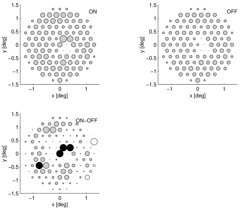
Figure 3: Comparison of the sky brightness for the ON and OFF source regions for supernova remnant G78.2+2.1 (a shell-type remnant located in a bright region of the galactic plane). In the top panels, the size of the circle is proportional to the RMS pedestal deviation for each PMT, scaled to a maximum value of 9.2 d.c. The bottom panel depicts the difference between the ON and OFF source observation, scaled to a maximum difference of 2.0 d.c. Positive differences are shown as filled circles, while open circles denote negative differences. The black circles show PMTs with a greater than 2.0 d.c. difference, due to the presence of bright stars in the ON source region.

An example of sky brightness is given in Figure 3 for the ON and OFF source regions of the supernova remnant G78.2+2.1 (see buckley98 for the results of TeV gamma-ray observations). For this object, located in a bright region of the galactic plane, the difference in sky brightness is quite large thus the application of software padding is essential. The results of the analysis of this extended object, with and without the application of software padding, will be presented later in this paper.

We characterize each Cherenkov image using a moment analysis reynolds93 . The roughly elliptical shape of the image is described by the length and width parameters. Its location and orientation within the FOV are given by the distance and $\alpha$ parameters, respectively. The asymmetry parameter, defined as the third moment of the light distribution, describes the skew of the image along its major axis. We also determine the two highest signals recorded by the PMTs (max1, max2) and the amount of light in the image (size). These parameters are defined in Table 1 and are depicted in Figure 4.

Table 1: Definition of image parameters, used to characterize the image shape and orientation in the FOV (see Figure 4).

Parameter	Definition
max1:	largest signal recorded by the PMTs.
max2:	second largest signal recorded by the PMTs.
size:	sum of all signals recorded.
centroid:	weighted center of the light distribution ($x_{c},y_{c}$).
width:	the RMS spread of light along the minor axis of the image;
	a measure of the lateral development of the shower.
length:	the RMS spread of light along the major axis of the image;
	a measure of the vertical development of the shower.
distance:	the distance from the centroid of the image to the center
	of the FOV.
$\alpha$:	the angle between the major axis of the image and a line
	joining the centroid of the image to the center of the
	FOV.
asymmetry:	the skewness of the light distribution relative to the
	image centroid.
disp:	the angular distance from the image centroid to the assumed
	arrival direction of the shower in the image plane.
$\theta$:	the angular distance from the arrival direction of the
	shower in the image plane and the center of the FOV.

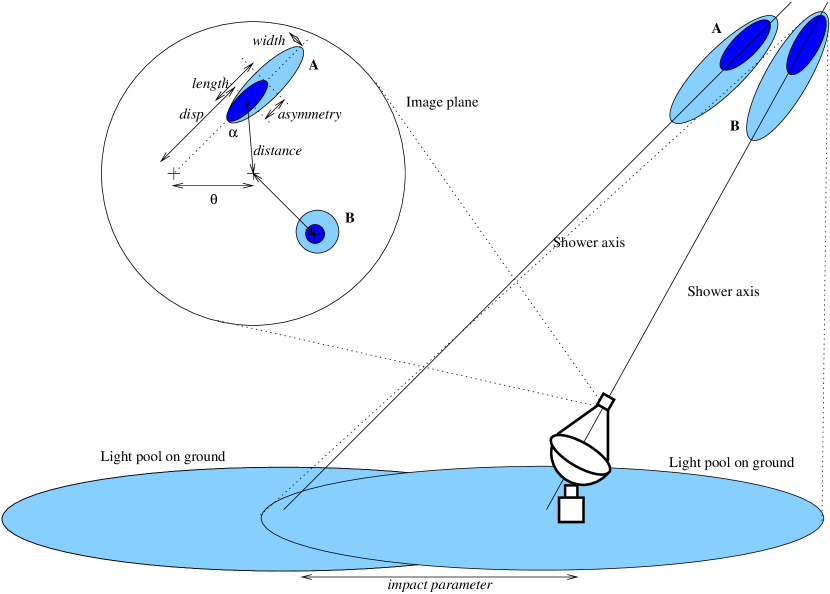
Figure 4: Depiction of the light produced by air showers. The image plane shows the definition of the Hillas parameters used to characterize each image.

3 Analysis Techniques

Gamma-ray events give rise to shower images which are preferentially oriented towards the source position in the image plane. These images are narrow and compact in shape, elongating as the impact parameter increases. They generally have a cometary shape with their light distribution skewed towards their source location in the image plane. Hadronic events give rise to images that are, on average, broader (due to the emission angles of pions in nucleon collisions spreading the shower), and longer (since the nucleon component of the shower penetrates deeper into the atmosphere) and are randomly oriented within the FOV. Utilizing these differences, a gamma-ray signal can be extracted from the large background of hadronic showers.

3.1 Traditional Methods

The standard gamma-ray selection method utilized by the Whipple Collaboration is the Supercuts criteria (see Table 2; cf., reynolds93 ; catanese95 ; lebohec2000 ). These criteria were optimized on contemporaneous Crab Nebula data giving the best sensitivity to point sources positioned at the center of the FOV. In an effort to remove background events triggered by single muons and night sky fluctuations, Supercuts incorporates pre-selection cuts on the size and on max1 and max2. The cuts on width and length select the more compact gamma-ray images and the cut on distance selects images for which the pointing angle $\alpha$ is well defined. The changes to the upper bounds of the length and distance cuts for the various cameras reflects the increasing FOV which results in less image truncation thereby allowing an accurate reconstruction of more distant images. A final cut on $\alpha$ selects images which are aligned towards the source position, assumed to be at the center of the FOV. A gamma-ray signal is detected as a statistically significant excess of events, which pass the above criteria, between ON source and OFF source observations. In the case when the source is not positioned at the center of the FOV, this technique is insensitive to any excess.

Table 2: Supercuts gamma-ray selection criteria. These criteria were optimized for each of the three camera configurations. Monte Carlo simulations indicate that for observations at zenith angles $<35^{\circ}$ this analysis results in an energy threshold of 350 GeV for the $3.0^{\circ}$ and $3.5^{\circ}$ camera FOV and 500 GeV for the $4.8^{\circ}$ camera FOV mohanty98 .

Supercuts (1995/1996)	Supercuts (1997)	Supercuts (1998)
$3.0^{\circ}$ FOV	$3.5^{\circ}$ FOV	$4.8^{\circ}$ FOV
pre-selection criteria
max1 $>$ 100 d.c.a	max1 $>$ 95 d.c.	max1 $>$ 78 d.c.
max2 $>$ 80 d.c.	max2 $>$ 45 d.c.	max2 $>$ 56 d.c.
size $>$ 400 d.c.	size $>$ 0 d.c.	size $>$ 0 d.c.
gamma-ray selection
$0.073^{\circ}<$ width $<0.15^{\circ}$	$0.073^{\circ}<$ width $<0.16^{\circ}$	$0.073^{\circ}<$ width $<0.16^{\circ}$
$0.16^{\circ}<$ length $<0.30^{\circ}$	$0.16^{\circ}<$ length $<0.33^{\circ}$	$0.16^{\circ}<$ length $<0.43^{\circ}$
$0.51^{\circ}<$ distance $<1.10^{\circ}$	$0.51^{\circ}<$ distance $<1.17^{\circ}$	$0.51^{\circ}<$ distance $<1.25^{\circ}$
$\alpha<15^{\circ}$	$\alpha<15^{\circ}$	$\alpha<10^{\circ}$
		asymmetry $>0^{\circ}$

a) d.c. = digital counts (1.0 d.c. $\approx$ 1.0 photoelectron).

3.2 Photon Arrival Direction

If the source position is ill-defined or if the source is extended, the traditional method becomes ineffective. As a result two different methods may be applied. In the first, the FOV is divided into a grid and each grid point is tested for an excess of events above background utilizing the Supercuts selection criteria given in Table 2 or using cuts which make use of asymmetry to break the pointing ambiguity and width/length to better localize the image. This method is described in detail in akerlof91 , fomin94 and buckley98 . In the second method, a unique arrival direction is determined thereby generating a TeV gamma-ray map of the FOV (see also lebohec98 for a description of an alternative method utilized by the Cherenkov Array at Thémis (CAT) group). The benefit of the second method is that it can be easily utilized in a search for extended or diffuse emission. This second method is described below.

By employing several features of gamma-ray induced showers, the arrival direction of a photon can be determined with the atmospheric Cherenkov technique, using a single telescope. Cherenkov light images of showers can be characterized as elongated ellipses with the major axis representing the projection of the shower trajectory along the image plane. The position of the source must lie along this axis near the tip of the light distribution corresponding to the initial interaction of the shower cascade. In addition, the position of the source must lie in the direction indicated by the asymmetry of the image. The elongation of a shower image and the angular distance between its centroid and the source position depend upon the impact parameter of the shower on the ground (see Figure 4). For small impact parameters, the image should have a form close to that of a circle and be positioned very near the source position in the focal plane fomin94 . For increasing impact parameter it should become elongated and have a form close to that of an ellipse and be positioned further from the source position in the focal plane as shown in Figure 4. The elongation of an image can be expressed as the ratio of its angular width and length. A simple form for the relationship between the elongation of an image and the angular distance between its centroid and the source position, disp, is

$$disp=\xi(1-\frac{width}{length})$$ (7)

where $\xi$ is a scaling parameter. A combination of these features provides a unique arrival direction for each gamma-ray event.

The value of disp depends on an unknown scaling factor $\xi$. Generally, $\xi$ will depend on the height of the shower in the atmosphere, the elevation of the detector on the ground, the zenith angle of the observation, parameters of the model of the atmosphere and the energy of the primary particle. For observations at small zenith angles ($<35^{\circ}$), and for the majority of events near the threshold of the instrument, the dependence on zenith angle and energy can be neglected. The value of $\xi$ will be further modified by the effect of the finite size of the camera in the focal plane giving rise to edge effects due to the truncation of images. Experimentally, $\xi$ is determined from data so that the calculated shower arrival directions line up with a known source position. For example, if a value of $\xi$ is chosen which is too small, then due to azimuthal symmetry, the arrival directions will circumvent the source location, similarly for values of $\xi$ too large. The optimum value of $\xi$ minimizes the spread in the angular distribution of events centered at the source position. The dependence of the angular spread of the arrival directions on the scaling factor $\xi$ is depicted in Figure 5. By minimizing the spread in the arrival directions the optimum angular resolution is achieved. This has the added advantage of increasing the signal to background ratio when determining an excess of events from a region.

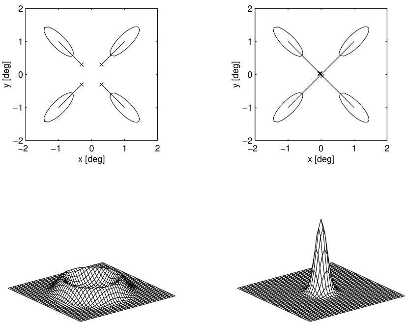
Figure 5: Conceptual depiction of the angular spread of event arrival directions. (Left) A value of $\xi$ which is too small so that the arrival directions circle the source location. (Right) The optimum value of $\xi$ minimizes the angular spread of arrival directions.

Data from the Whipple 10 m gamma-ray telescope is used to optimize the value of $\xi$. We include data from each of the three cameras (see Table 3), taken on established sources, positioned at the center of the FOV which should appear point-like. First, events are selected as gamma-like based on the angular width and length criteria given in Table 2. No selection on distance or $\alpha$ is made. Secondly, the arrival direction of each event is determined utilizing Equation 7. Next, each arrival direction is corrected for the rotation of the FOV, due to the altitude-azimuth mount used by the Whipple 10 m telescope, by de-rotating the position to zero hour angle. These corrected arrival directions are binned on a two dimensional grid of bin size $0.1^{\circ}$x$0.1^{\circ}$. Figure 6 shows examples of the binned excess arrival directions, for data taken on Markarian 501 (see Table 3), projected along the x-axis, for two values of the scaling parameter $\xi$. The excess shows the difference between accumulated ON source events and corresponding OFF source control data.

Table 3: Data used to optimize the scaling parameter $\xi$.

Camera	Source	Observation	Total ON
FOV	name	period	source time (mins)
$3.0^{\circ}$	Markarian 421 punch92	1995	523.2
$3.5^{\circ}$	Markarian 501 quinn96	1997	471.6
$4.8^{\circ}$	Crab Nebula weekes89	1998	845.9

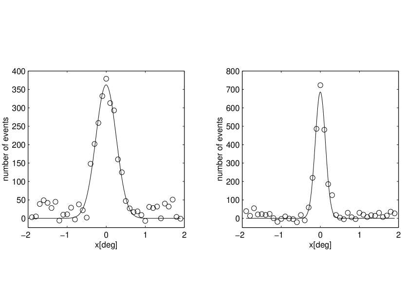
Figure 6: Binned excess arrival directions projected along the x-axis for scaling factor $\xi$ of 1.20 (left) and 1.78 (right).

The spread in arrival directions for each value of $\xi$ is determined by fitting a Gaussian function of standard deviation $\sigma$ to the binned excess. The results are depicted in Figure 7. The minimum spread occurs at a value of $\xi=1.78^{\circ},1.78^{\circ},1.65^{\circ}$ for the $3.0^{\circ},3.5^{\circ}$ and $4.8^{\circ}$ camera FOV respectively. The effect of the decreasing optimum value of $\xi$ with increasing FOV is the result of less image truncation imposed by the larger camera. This effect is also evident in the upper bound of the optimum length cut used to select gamma-ray images (see Table 2). The minimum spread is a measure of the optimum angular resolution, or point spread function (PSF) of the technique and corresponds to $\sigma=0.11^{\circ},0.13^{\circ}$ and $0.12^{\circ}$ respectively.

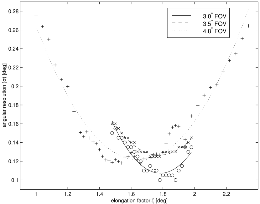
Figure 7: Variation of the spread in excess arrival directions with elongation scaling factor $\xi$. The data was fitted by a quadratic function, shown by the curves, for the purpose of determining the minimum spread.

4 Results

The determination of a photon’s arrival direction enables the search for emission from anywhere within the camera’s FOV. When the source position is known, a gamma-ray signal is detected as an excess of events, between corresponding ON and OFF source observations, originating from the source direction. Firstly, events are selected as gamma-like based on the angular width and length criteria given in Table 2 and their arrival directions determined as described above. Secondly, the radial distance from the arrival direction to the source position, $\theta$, is calculated and binned in $0.02^{\circ}$ intervals. The results of data taken with the three cameras are shown in Figure 8. The area of exposure for each bin increases with greater radial distance, therefore each bin contents have been divided by the area of the annulus defined by the bin boundaries. The physical interpretation of such a distribution is the surface brightness of an extended object.

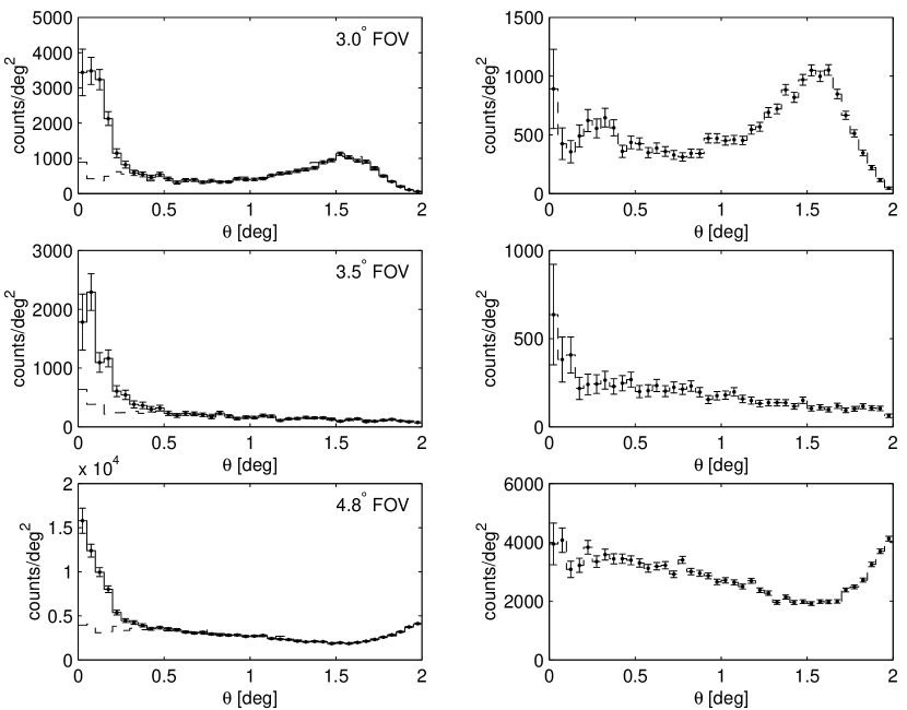
Figure 8: Distribution of the radial distance of photon arrival directions from the center of the FOV, $\theta$, for data taken with all three cameras. (Left) The solid line depicts the ON source observation and the dashed line shows the results of an equivalent amount of time taken on a corresponding OFF source region. (Right) The dashed line shows only the OFF source observation. The presence of a rise in the number of events near the edge of the FOV is absent from the $3.5^{\circ}$ camera results due to less image truncation imposed by the smaller triggering FOV (see Figure 1).

4.1 Aperture Selection Criteria

For each data set depicted in Figure 8, an excess gamma-ray signal is apparent in the ON source observation (solid line) when compared to the OFF source observation (dotted line) and the excess is confined to small values of $\theta$. The angular extent of the signal is similar for each camera, consistent with the results of the optimized angular resolution. The results of the OFF source observations illustrate a background which appears uniform for small values of $\theta$ with a gradual decline due to the finite size of the camera. In the $3.0^{\circ}$ and $4.8^{\circ}$ cameras, all PMTs enter into the trigger (all of the way out to the edge of the FOV), whereas in the $3.5^{\circ}$ camera only the inner 91 out of the 151 PMTs enter into the trigger (see Figure 1). Thus in the $3.0^{\circ}$ and $4.8^{\circ}$ cameras there are a number of background cosmic-ray events which lie on the edge of the camera and which are distorted by image truncation. This truncation tends to produce images whose major axes make an angle of $\alpha=90^{\circ}$ and results in a significant rise in the number of events collected at large values of $\theta$. This rise is not apparent in the results from the $3.5^{\circ}$ camera. The selection of events consistent with the position of the source is accomplished by counting the number of events within a circular aperture of radius $\theta_{c}$ centered at the source position. The optimum value of $\theta_{c}$ is determined using data taken with the $4.8^{\circ}$ camera. The results are shown in Figure 9 and yield an optimum selection criteria of $\theta<0.22^{\circ}$. This selection criteria can be applied to the data for all camera configurations owing to the similar radial extent of the gamma-ray signal. When the angular extent of the source is of the order, or greater than the resolution of the technique, the size of the circular aperture can be adjusted to the size of the emission region. In doing so more background is included, hence sensitivity is diminished. In background dominated counting statistics, the sensitivity of a detector will be proportional to $1/\sqrt{background}$. If we neglect the gradual decline in the background with increasing angular offset, the sensitivity of an atmospheric Cherenkov telescope utilizing this method will scale as $1/\theta_{c}$.

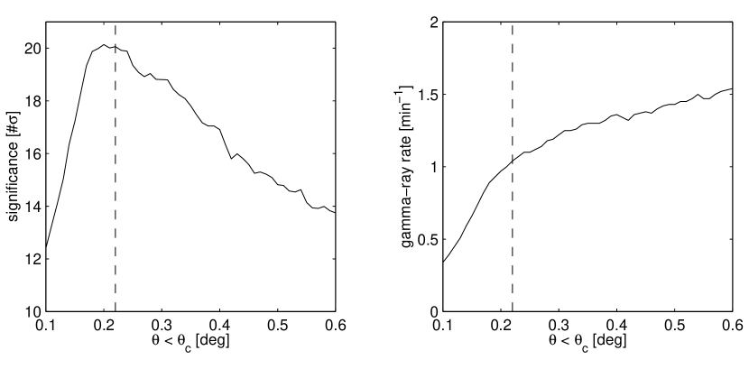
Figure 9: Results of the optimization of the selection criteria $\theta<\theta_{c}$. (Left) The solid line shows the statistical significance of the excess between ON and corresponding OFF source observations. The dashed line shows the value of the optimum cut chosen, approximately the center of the peak. (Right) The solid line shows the gamma-ray signal obtained.

TeV gamma-ray observations of the supernova remnant G78.2+2.1, reported by the Whipple Collaboration in buckley98 , is an example of an extended source. The expanding shell of the supernova explosion subtends an angle of approximately $0.5^{\circ}$. The distribution of $\theta$, for a subset of the data reported in buckley98 , is given in Figure 10. In the search for a gamma-ray signal, a circular aperture was chosen to encompass the size of the emission region plus twice the angular resolution to account for smearing of the edges. As shown in Figure 10, no significant excess was obtained. Also shown is an example of a false signal resulting from biases due to sky brightness differences. Without the application of software padding, the brighter ON source region yields a greater number of background events selected as gamma-rays resulting in a significant excess between the ON and OFF source observations.

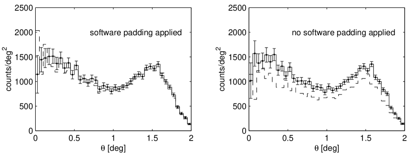
Figure 10: Results of TeV gamma-ray observations of the diffuse supernova remnant G78.2+2.1. Each panel depicts the distribution of $\theta$ for the ON (solid line and error bars) and OFF (dashed line) source observations. The left panel depicts results utilizing software padding. The right panel depicts results without the application of software padding.

4.2 Gamma-ray Collection Efficiency

We compare the gamma-ray collection efficiency and background rejection of the aperture selection method with the traditional Supercuts criteria using data taken on the Crab Nebula, the standard candle for TeV gamma-ray astronomy. The results from the three camera configurations are given in Table 4. The data collected with the $3.0^{\circ}$ camera was taken in January - February 1995. Like the traditional Supercuts criteria, the aperture selection includes events which are oriented towards the center of the FOV. However, the aperture selection has two further constraints in that events must be skewed towards the center of the FOV and must be elongated in proportion to the impact parameter on the ground. These additional criteria result in greater background rejection compared with Supercuts. Results from the $3.0^{\circ}$ camera indicate a reduced gamma-ray collection efficiency due to image truncation imposed by the smaller FOV. Truncated images reduce the effectiveness of the asymmetry parameter by clipping the tails of the light distribution which defines the skewness of the image. Data collected with the $3.5^{\circ}$ and $4.8^{\circ}$ cameras were taken in January - February 1997 and November 1998 - January 1999 respectively. First note that for the data taken with the $4.8^{\circ}$ FOV camera, a degradation of mirror reflectivity and lack of light cones resulted in an increased energy threshold and lower count rate on the Crab Nebula. Despite the increased threshold this data can still be used to judge the effectiveness of the extended camera. These results not only show the same improvement in background rejection over the traditional Supercuts criteria, but indicate similar gamma-ray collection efficiency. This results in a marginal increase in sensitivity of the aperture selection criteria over traditional Supercuts.

Table 4: Comparison of Supercuts with Aperture selection criteria using data taken on the Crab Nebula (the standard candle for TeV astronomy).

Selection	Observation	ON	OFF	Significance	Gamma-ray
criteria	duration	source	source	$\sigma$/hr	rate
	(min)	counts	counts		(min-1)
$3.0^{\circ}$ FOV
Supercuts	246.9	948	408	7.2	$2.2\pm 0.1$
Aperture		353	77	6.6	$1.12\pm 0.08$
$3.5^{\circ}$ FOV
Supercuts	304.6	1654	871	6.9	$2.6\pm 0.2$
Aperture		790	211	8.1	$1.9\pm 0.1$
$4.8^{\circ}$ FOV
Supercuts	845.9	1683	778	4.8	$1.07\pm 0.06$
Aperture		1404	524	5.3	$1.04\pm 0.05$

4.3 The Sky in TeV Gamma Rays

If the position of the source is unknown but assumed to be in the FOV, a two dimensional grid of bin size $0.1^{\circ}$x$0.1^{\circ}$ is constructed. Events are first selected as gamma-like based on the angular width and length criteria given in Table 2, and their arrival directions determined as described above. Next, the contents of each grid point within the optimum cut on the radial distance from the arrival direction is incremented by one. Figure 11 shows the accumulated grid contents for data taken with the $3.5^{\circ}$ camera. Conceptually, this performs a type of image smoothing about the calculated photon arrival direction resulting in an oversampled gamma-ray map which is tuned to the search for point sources anywhere within the camera’s FOV. The statistical significance of excess events between ON and corresponding OFF source observations is calculated for each grid point using the method of li83 . The use of Poissonian statistics is valid in this case because grid points are incremented by unity. However, one must be careful in interpreting the significance. To be precise, the test statistic calculated at each grid point can only be interpreted as significance if there was a prior hypothesis for gamma-ray emission from a point source at that position. Otherwise, the number of independent grid points tested, or trials factor, must be taken into account thereby degrading the significance. For example, for a grid ($3.9^{\circ}$ FOV divided into $0.1^{\circ}$ bins) with 1521 grid points (not independent) we have effectively 324 trials and expect on average one $3\sigma$ excess.

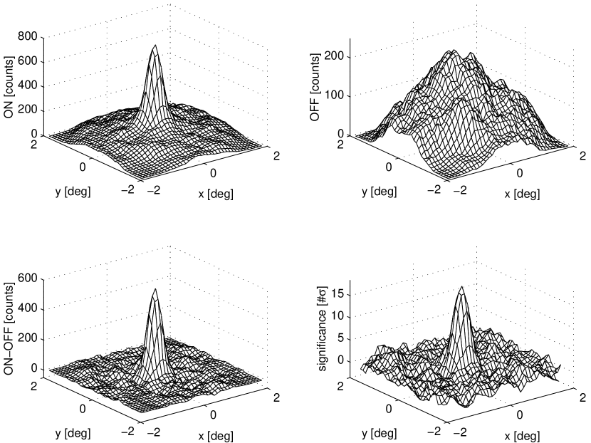
Figure 11: Shown are the accumulated grid contents for the observations taken with the $3.5^{\circ}$ camera. (Top left) ON source data given in Table 3. (Top right) The corresponding OFF source data. (Bottom left) The difference in counts and significance (Bottom right).

An example of a TeV gamma-ray image of a region of sky (the supernova remnant G78.2+2.1), found to be devoid of a gamma-ray signal, is shown in Figure 12. The image shows several $2\sigma$ excesses and one $3\sigma$ excess. However, without a prior hypothesis for gamma-ray emission from a point source at these positions a trials factor for the number of independent grid points must applied, resulting in a reduction in significance. Also shown in Figure 12 is an example of a false signal resulting from biases due to sky brightness differences. The region of the image showing the greatest excesses appear well correlated with the sky brightness difference between the ON and OFF source regions as depicted in Figure 3.

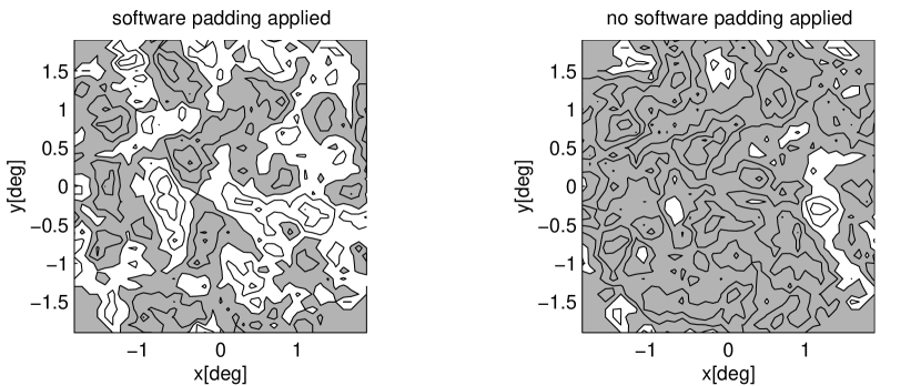
Figure 12: Results of TeV gamma-ray observations of the supernova remnant G78.2+2.1. The contours are proportional to the statistical significance of the smoothed excess gamma-ray events and increment by one standard deviation. Contours depicting positive excess are shaded in gray. The left panel depicts results utilizing software padding. The right panel depicts results without the application of software padding.

To test the efficacy of the technique and measure the efficiency and sensitivity away from the center of the FOV, we analyzed data taken on the Crab Nebula which was offset in declination. The results are shown in Figures 13,14 and 15 for the $3.0^{\circ},3.5^{\circ}$ and $4.8^{\circ}$ cameras respectively. The contours are proportional to the statistical significance of the excess between the ON and OFF source data. The peak excess and detected gamma-ray rates are given in Table 5.

Table 5: Results of data taken on the Crab Nebula offset in declination.

Offset	Observation	Standard deviation	Significance	Gamma-ray
(∘)	duration (min)	of PSF (∘)	#$\sigma$	rate (min-1)
$3.0^{\circ}$ FOV
0.00	246.9	0.15	13.4	$1.08\pm 0.08$
0.37	83.0	0.13	6.8	$0.9\pm 0.1$
$3.5^{\circ}$ FOV
0.00	304.6	0.13	18.3	$1.9\pm 0.1$
0.50	54.8	0.13	6.1	$1.2\pm 0.2$
1.00	83.2	0.15	6.3	$0.8\pm 0.1$
1.50	138.5	0.11	4.3	$0.35\pm 0.08$
$4.8^{\circ}$ FOV
0.00	845.9	0.12	20.1	$1.04\pm 0.05$
1.00	55.4	0.10	4.5	$0.7\pm 0.2$
1.50	106.7	0.14	3.7	$0.35\pm 0.09$

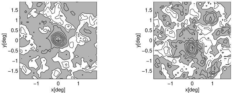
Figure 13: Results of the observations taken with $3.0^{\circ}$ camera on the Crab Nebula, centered in the FOV (Left) and offset in declination by 22 arcminutes (Right), corresponding to observation times of 247 min and 83 min respectively. The contours are proportional to the statistical significance of the smoothed excess gamma-ray events and increment by two standard deviations (Left) and one standard deviation (Right). Contours depicting positive excess are shaded in gray. The cross indicates the position of the Crab Nebula and the systematic pointing uncertainty.

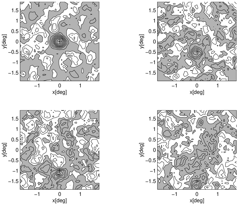
Figure 14: Results of the observations taken with $3.5^{\circ}$ camera on the Crab Nebula, centered in the FOV (Top Left) and offset in declination by $0.5^{\circ}$ (Top Right), $1.0^{\circ}$ (Bottom Left) and $1.5^{\circ}$ (Bottom Right), corresponding to observation times of 305 min, 55 min, 83 min and 138 min respectively. The contours are proportional to the statistical significance of the smoothed excess gamma-ray events and increment by two standard deviations for the centered observation and by one standard deviation for the offset observations. Contours depicting positive excess are shaded in gray. The cross indicates the position of the Crab Nebula and the systematic pointing uncertainty.

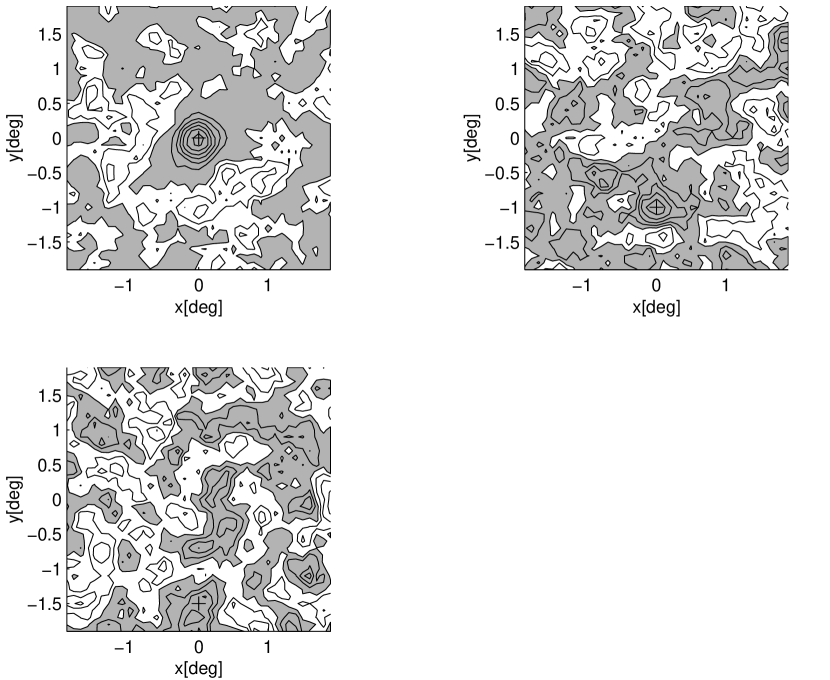
Figure 15: Results of the observations taken with $4.8^{\circ}$ camera on the Crab Nebula, centered in the FOV (Top Left) and offset in declination by $1.0^{\circ}$ (Top Right) and $1.5^{\circ}$ (Bottom Left), corresponding to observation times of 846 min, 55 min and 107 min respectively. The contours are proportional to the statistical significance of the smoothed excess gamma-ray events and increment by three standard deviations for the centered observation and by one standard deviation for the offset observations. Contours depicting positive excess are shaded in gray. The cross indicates the position of the Crab Nebula and the systematic pointing uncertainty.

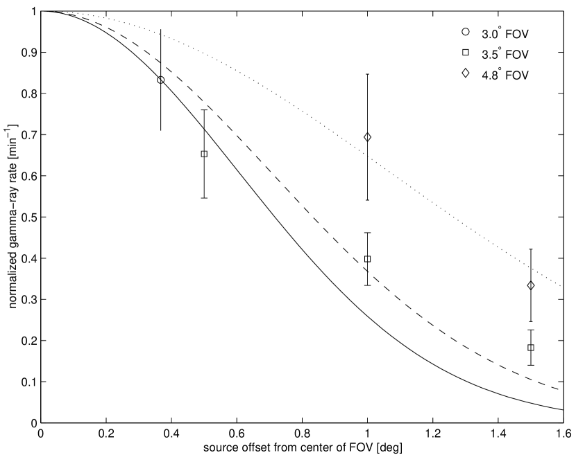
Figure 16: The measured gamma-ray rate from the Crab Nebula normalized to the rate at the center of the FOV. The curves indicate the general trend of the data.

The results show that the technique is sensitive to a gamma-ray signal offset from the center of the FOV. For the $3.5^{\circ}$ and $4.8^{\circ}$ cameras, the Crab Nebula was detected with a sensitivity of approximately $3\sigma$/hr for an offset of $1.5^{\circ}$. The derived position of the Crab Nebula was within the $0.1^{\circ}$ pointing accuracy of the Whipple 10 m telescope for offsets less than $1.0^{\circ}$. We note that there appears to be a small systematic shift of the derived position of the Crab Nebula for the $1.0^{\circ}$ and $1.5^{\circ}$ offsets for the data taken with the $3.5^{\circ}$ camera and for the $1.5^{\circ}$ offsets for the data taken with the $4.8^{\circ}$ camera. The shift is most likely due to the inclusion of truncated images as the source moves closer to the edge of the FOV. The spread of events about the derived source position was determined by fitting a Gaussian function to the unsmoothed binned excess. The results indicate that the PSF is approximately constant over the FOV of the camera and thus not dependent on the optical properties of the reflector which degrade with increasing angular offset.

As the gamma-ray source moves away from the center of the camera, less of the Cherenkov light pool falls on the detector at a given impact parameter. This has the effect of reducing the collection area for gamma-rays. The measurements of the gamma-ray rate from the Crab Nebula at increasing angular offset is a direct measure of this reduction as shown in Figure 16. The effective FOV, which we arbitrarily define as the radius corresponding to a 50% efficiency, appears to scale linearly with camera physical FOV, at least up to the range of offsets and camera sizes included in these results. For example, a camera with a physical FOV of $6.0^{\circ}$ would have an effective FOV double that of a camera with a $3.0^{\circ}$ FOV. Moreover, by doubling the diameter of the FOV a fourfold increase in sensitive area for sources offset from the center of the FOV is realized.

5 Conclusion

We have described a method of atmospheric Cherenkov imaging which reconstructs the unique arrival direction of TeV gamma-rays using a single telescope. This method is derived empirically making use of the Crab Nebula as a standard candle to optimize the angular resolution of the technique. This allows a selection of events based on the position of a source anywhere within the telescope’s FOV. We found that such a selection yields similar sensitivity and collection efficiency to the traditional Supercuts criteria utilized by the Whipple Collaboration. However, as demonstrated, the technique is easily applicable to sources offset from the center of the FOV or sources of extended emission.

References

- (1) T.C. Weekes, et al., ApJ, 174 (1972) 165.
- (2) M.F. Cawley, et al., Exper. Astr., 1 (1990) 173.
- (3) A.M. Hillas, Proc. 19th ICRC, 3 (La Jolla, USA, 1985) 445.
- (4) D.J. Fegan, et al., Proc. Towards a Major Atmospheric Cherenkov Detector III (Tokyo, Japan, 1994) 149.
- (5) V. Connaughton, et al., APh, 8 (1998) 179.
- (6) J.H. Buckley, et al., A&A, 329 (1998) 639.
- (7) S. Le Bohec, et al., ApJ, in press (2000).
- (8) M.F. Cawley, Proc. Towards a Major Atmospheric Cherenkov Detector II (Calgary, Canada, 1993) 176.
- (9) P.T. Reynolds, et al., ApJ, 404 (1993) 206.
- (10) M. Catanese, et al., Proc. Towards a Major Atmospheric Cherenkov Detector IV (Padova, Italy, 1995) 335.
- (11) G. Mohanty, et al., APh, 9 (1998) 15.
- (12) C.W. Akerlof, et al., ApJ, 377 (1991) L97.
- (13) V.P. Fomin, et al., APh, 2 (1994) 137.
- (14) S. Le Bohec, et al., Nucl. Instr. and Meth. A, 416 (1998) 425.
- (15) M. Punch, et al., Nature, 358 (1992) 477.
- (16) J. Quinn, et al., ApJ, 456 (1996) L83.
- (17) T.C. Weekes, et al., ApJ, 342 (1989) 379.
- (18) T.P. Li and Y.Q Ma, ApJ 272 317.