A JET MODEL FOR THE AFTERGLOW EMISSION FROM GRB 000301C

Abstract

We present broad-band radio observations of the afterglow of GRB 000301C, spanning from 1.4 to 350 GHz for the period of 3 to 83 days after the burst. This radio data, in addition to measurements at the optical bands, suggest that the afterglow arises from a collimated outflow, i.e. a jet. To test this hypothesis in a self-consistent manner, we employ a global fit and find that a model of a jet, expanding into a constant density medium (ISM+jet), provides the best fit to the data. A model of the burst occurring in a wind-shaped circumburst medium (wind-only model) can be ruled out, and a wind+jet model provides a much poorer fit of the optical/IR data than the ISM+jet model. In addition, we present the first clear indication that the reported fluctuations in the optical/IR are achromatic with similar amplitudes in all bands, and possibly extend into the radio regime. Using the parameters derived from the global fit, in particular a jet break time, $t_{jet}\approx 7.5$ days, we infer a jet opening angle of $\theta_{0}\approx 0.2$, and consequently the estimate of the emitted energy in the GRB itself is reduced by a factor $\sim$50 relative to the isotropic value, giving $E\approx 1.1\times 10^{51}$ ergs.

1. Introduction

GRB 000301C is the latest afterglow to exhibit a break in its optical/IR light curves. An achromatic steepening of the light curves has been interpreted in previous events (e.g. Kulkarni et al. 1999a ; Harrison et al. (1999)) as the signature of a jet-like outflow (Rhoads (1999); Sari Piran & Halpern (1999)), produced when relativistic beaming no longer “hides” the non-spherical surface, and when the ejecta undergo rapid lateral expansion. The question of whether the relativistic outflows from gamma-ray bursts (GRBs) emerge isotropically or are collimated in jets is an important one. The answer has an impact both on estimates of the GRB event rate and the total emitted energy — issues that have a direct bearing on GRB progenitor models.

An attempt by Rhoads and Fruchter (2000) to model this break using only the early time ($\Delta t\lesssim 14$ days) optical/IR data has led to a jet interpretation of the afterglow evolution, but with certain peculiar aspects, such as a different jet break time at R band than at K’ band. However, subsequent papers by Masetti et al. (2000), and Sagar et al. (2000), with larger optical data sets, pointed out that there are large flux density variations ($\sim 30\%$) on timescales as short as a few hours, superposed on the overall steepening of the optical/IR light curves. While the origin of these peculiar fluctuations remains unknown, it is clear that they complicate the fitting of the optical/IR data, rendering some of the Rhoads and Fruchter results questionable.

In this paper we take a different approach. We begin by presenting radio measurements of this burst from 1.4 GHz to 350 GHz, spanning a time range from 3 to 83 days after the burst. These radio measurements, together with the published optical/IR data, present a much more comprehensive data set, which is less susceptible to the effects of the short-timescale optical fluctuations. We then use the entire data set to fit a global, self-consistent jet model, and derive certain parameters of the GRB from this model. Finally, we explore the possibility of a wind, and wind+jet global fit to the data, and compare our results with the conclusions drawn in the previous papers.

2. Observations

Radio observations were made from 1.43 GHz to 350 GHz, at a number of facilities, including the James Clark Maxwell Telescope (JCMT), the Institut f$\ddot{\rm u}$r RadioAstronomie im Millimeterbereich (IRAM ), the Owens Valley Radio Observatory Interferometer (OVRO), the Ryle Telescope and the (Very Large Array (VLA). A log of these observations and the flux density measurements are summarized in Table 1. With the exception of IRAM, we have detailed our observing and calibration methodology in Kulkarni et al. (1999) and Frail et al. (2000).

Observations at IRAM were made using the Max-Planck Millimeter Bolometer (MAMBO; Kreysa et al. 1999) at the IRAM 30-m telescope on Pico Veleta, Spain. Observations were made in standard on-off mode. Gain calibration was performed using observations of Mars, Uranus, and Ceres. We estimate the calibration to be accurate to 15%. Using the MOPSI software package (Zylka 1998), the temporally correlated variation of the sky signal (sky-noise) was subtracted from all bolometer signals. The source was observed on March 4, 5, and 9 under very stable atmospheric conditions, and on March 6 with high atmospheric opacity. From March 24 to 26, the source was briefly re-observed three times for a total on+off integration time of 2000 sec, but no signal was detected.

3. The Data

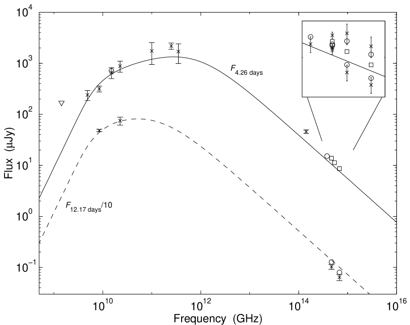
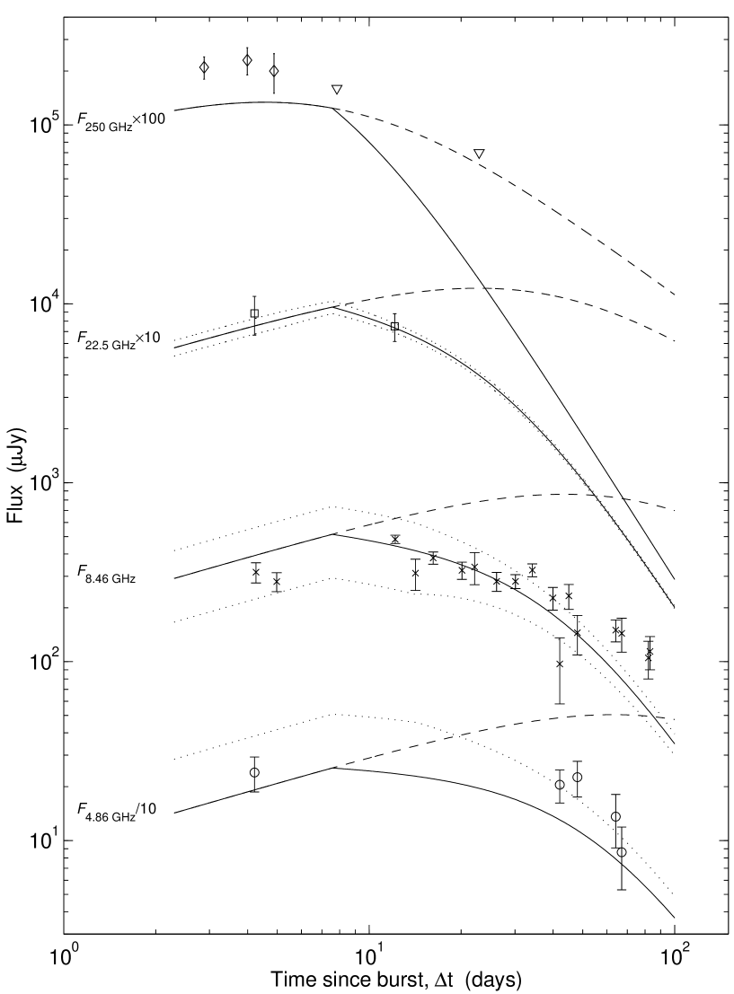
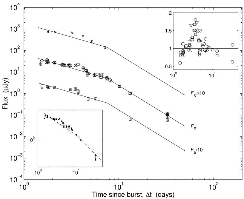
In Figure 1 we present broad-band spectra from March 5.66 UT ($\Delta t\approx 4.25$ days) and March 13.58 UT ($\Delta t\approx 12.17$ days). Radio light curves at 4.86, 8.46, 22.5, and 250 GHz from Table 1 are presented in Figure 2, while optical/IR curves are shown in Figure 3.

The quoted uncertainties in the flux densities given in Table 1 report only measurement error and do not contain an estimate of the effects of interstellar scattering, which is known to be significant for radio afterglows (e.g. Frail et al. (1999)). We can get some guidance on the expected magnitude of the ISS-induced modulation of our flux density measurements (in time and frequency) using the models developed by Taylor and Cordes (1993), Walker (1998), and Goodman (1997).

From the Galactic coordinates of GRB 000301C  (l,b)=($48.7^{\circ},44.3^{\circ}$), we find, using the Taylor and Cordes model, that the scattering measure is $SM_{-3.5}\approx 0.7$. The distance to the scattering screen, $d_{scr}$, is one half the distance through the ionized gas layer, $d_{scr}=(hz/2)({\rm sin}b)^{-1}\approx 0.72$ kpc, using $hz\approx 1$ kpc. From Walker’s analysis, the transition frequency between weak and strong scintillation is then given by $\nu_{0}=5.9SM_{-3.5}^{6/17}d_{scr}^{5/17}\approx 4.7$ GHz. Goodman (1997) uses the same scalings, but with a different normalization for the transition frequency, giving a larger value, $\nu_{0}\approx 8.3$ GHz. In this section we follow Walker’s analysis, and note that the numbers from Goodman will give different results.

For frequencies larger than the transition frequency the modulation index (i.e. the r.m.s. fractional flux variation) is $m_{\nu}=(\nu_{0}/\nu)^{17/12}$, and the modulation timescale in hours is $t_{\nu}\approx 6.7(d_{scr}/\nu)^{1/2}$. From this analysis we find that the modulation index is of order 0.4 at 8.46 GHz, 0.2 at 15 GHz, 0.10 at 22.5 GHz, and is negligible at higher frequencies. The modulation timescales are of order 2.0 hours at 8.46 GHz, 1.5 hours at 15 GHz, and 1.2 hours at 22.5 GHz. It is important to note that factor 2 uncertainties in the scattering measure allow the modulation index to vary by $\sim 50\%$.

At these frequencies the expansion of the fireball will begin to “quench” the ISS when the angular size of the fireball exceeds the angular size of the first Fresnel zone, $\theta_{F}=8(d_{scr}\nu_{GHz})^{-1/2}\mu$as. To describe the evolution of the source size with time, we have used an expanding jet model (see Frail et al. (1999)), with the factor $(E_{52}/n_{1})^{1/8}$ assumed to be of order unity, which gives $\theta_{s}\approx 3.1(\Delta t_{d}/15)^{1/2}\mu{\rm as}$. Once the source size exceeds the Fresnel size (after approximately two weeks at 8.46 GHz), the modulation index has to be corrected by a factor $(\Delta t_{d}/15)^{-7/12}$.

The measurements at 4.86 GHz occur near the transition frequency and we therefore expect $m_{4.86}$ to be large $\sim 0.65-1.0$. At 1.43 GHz the observations were made in the strong regime of ISS where we expect both refractive and diffractive scintillation. Point source refractive scintillation at 1.43 GHz has a modulation index $m_{1.43,r}=(\nu/\nu_{0})^{17/30}\approx 0.5$, with a timescale of $t_{1.43,r}\approx 2(\nu_{0}/\nu)^{11/5}\approx 1$ day. The refractive ISS is “quenched” when the angular size of the source is larger than $\theta_{r}=\theta_{F0}(\nu_{0}/\nu)^{11/5}$, where $\theta_{F0}$ is the angular size of the first Fresnel zone at $\nu_{0}=4.7$ GHz. As with weak scattering, the modulation index has to be corrected by a factor $(\Delta t_{d}/15)^{-7/12}$ after this point. The diffractive scintillation has a modulation index $m_{1.43,d}=1$, and a timescale, $t_{1.43,d}\approx 2(\nu/\nu_{0})^{6/5}\approx 0.5$ hrs $\ll t_{1.43,r}$. The source can no longer be approximated by a point source when its angular size exceeds $\theta_{d}=\theta_{F0}(\nu/\nu_{0})^{6/5}$, and correspondingly the modulation index has to be corrected by a factor $(\Delta t_{d}/15)^{-1/2}$.

The redshift of GRB 000301C was measured using the Hubble Space Telescope to be 1.95$\pm$0.1 by Smette et al. (2000) and was later refined by Castro et al. (2000) using the Keck II 10-m Telescope to a value of 2.0335$\pm$0.0003. The combined fluence measured by the GRB detector on board the Ulysses satellite, and the X-ray/gamma-ray Spectrometer (XGRS) on board the Near Earth Asteroid Rendezvous (NEAR) satellites, in the 25-100 keV and $>$100 keV bands was $\sim$4$\times 10^{-6}$ erg/cm². Using the cosmological parameters $\Omega_{0}$=0.3, $\Lambda_{0}$=0.7 and $H_{0}$=65 km/sec/Mpc, we find that the isotropic $\gamma$-ray energy release from the GRB was $E_{iso}\approx 5.4\times 10^{52}$ ergs.

4. A Self-Consistent Jet Interpretation

According to the standard, spherical GRB model, the optical light curves should obey a simple power-law decay, $F_{\nu}\propto t^{-\alpha}$, with $\alpha$ changing at most by 1/4 as the electrons age and cool (Sari, Piran, & Narayan 1998). From Figure 3 it is evident that the optical light curves steepen substantially ($\Delta\alpha>1/4$) between days 7 and 8, which indicates that this burst cannot be described within this standard model of an expanding spherical blast wave. This break can be attributed to a jet-like or collimated ejecta (Rhoads 1999; Sari, Piran, & Halpern 1999).

The jet model of GRBs predicts the time evolution of flux from the afterglow, and of the parameters $\nu_{a}\propto t^{-1/5}$, $\nu_{m}\propto t^{-2}$, and $F_{\nu,max}\propto t^{-1}$. This model holds for $t>t_{jet}$, where $t_{jet}$ is defined by the condition $\gamma(t_{jet})\sim\theta_{0}^{-1}$. Prior to $t_{jet}$ the time evolution of the afterglow is described by a spherically expanding blast wave, with the scalings $\nu_{a}\propto$ const., $\nu_{m}\propto t^{-3/2}$, and $F_{\nu,max}\propto$ const. In this paper we designate this model as ISM+jet. Throughout the analysis we assume that the cooling frequency, $\nu_{c}$, lies above the optical band for the entire time period under discussion in this paper.

At any point in time the spectrum is roughly given by the broken power law $F_{\nu}\propto\nu^{2}$ for $\nu<\nu_{a}$, $F_{\nu}\propto\nu^{1/3}$ for $\nu_{a}<\nu<\nu_{m}$, and $F_{\nu}\propto\nu^{-(p-1)/2}$ for $\nu>\nu_{m}$, where $p$ is the electron power law index. To globally fit the entire radio and optical/IR data set we employed the smoothed form of the broken power law synchrotron spectrum, calculated by Granot, Piran, and Sari (1999a,b). With this approach we treat $t_{jet}$, $p$, and the values of $\nu_{a}$, $\nu_{m}$, and $F_{\nu,max}$ at $t=t_{jet}$ as free parameters. This method forces $t_{jet}$ to have the same value at all frequencies. We find the following values for the burst parameters: $t_{jet}=7.5\pm 0.5$ days, $p=2.70\pm 0.04$, $\nu_{a}(t=t_{jet})=8.3\pm 1.8$ GHz, $\nu_{m}(t=t_{jet})=(3.0\pm 0.3)\times 10^{11}$ Hz, $F_{\nu,max}(t=t_{jet})=2.7\pm 0.2$ mJy, where the errors are derived from the diagonal elements of the correlation matrix. We note that there is substantial covariance between some of the parameters and therefore these error estimates should be treated with caution. From our fit the asymptotic temporal decay slopes of the optical light curves are $p$ we find $\alpha_{1}=-3(p-1)/4=-1.28$ for $t<t_{jet}$, and $\alpha_{2}=-p=-2.70$ for $t>t_{jet}$. The fits are shown in figures 1, 2, and 3.

The total value of $\chi^{2}$ for the global fit is poor. We obtain $\chi^{2}=450$ for 94 degrees of freedom. The bulk of this value, 340, comes from the 61 optical data points, and is the result of the fluctuations, which are not accounted for by our model. The radio data contribute a value of 110 to $\chi^{2}$ for $38$ data points. This is probably the result of scintillation. If we increase the errors to accommodate for the expected level of scintillation (see §3) we obtain a good fit with $\chi_{radio}^{2}=39/33$ degrees of freedom.

From figure 1 it is clear that the global fit accurately describes the broad-band spectra from days 4.26 ($<t_{jet}$) and 12.17 ($>t_{jet}$), with a single value of $p=2.70$, which rules out the possibility that the steepening of the light curves at $t=t_{jet}$ is the result of a time-varying $p$.

Trying to model the data using the approach outlined above, but for a wind-shaped circumburst medium results in a poor description of the data, because the wind model does not exhibit a break, although one is clearly seen in the optical data. As a result, the model fit is too low at early times, and too high at late times relative to the data (see insert in figure 3). The value of $\chi^{2}$ for the wind model relative to the ISM+jet model described above is $\chi^{2}_{wind}/\chi^{2}_{ISM+jet}\sim 3$. Therefore, a wind-shaped model can be ruled out as a description of the afterglow of GRB 000301C.

A jet evolution combined with a wind-shaped circumburst medium provides a more reasonable fit than a wind only model. The wind evolution of the fireball will only be manifested for $t<t_{jet}$ since once $\gamma(t_{jet})\approx\theta_{0}^{-1}$ the jet will expand sideways and appear to observers as if it were expanding into a constant density medium (Chevalier & Li 1999b; Livio & Waxman 1999). The resulting parameters from such a fit differ considerably from the parameters for the ISM+jet model quoted above, and the relative value of $\chi^{2}$ between the two models is $\chi^{2}_{wind+jet}/\chi^{2}_{ISM+jet}\sim 2$. This model suffers from a serious drawback in its description of the optical/IR light curves. Because the predicted decay of these light curves prior to $t_{jet}$ is steeper than in the ISM+jet model, the model fit, from 2 days after the burst up to the break time, is too low relative to the data (see insert in figure 3).

The approach outlined above, which uses one power law temporal evolution of $\nu_{a}$, $\nu_{m}$, and $F_{\nu,max}$ before $t_{jet}$, and a different power law evolution after $t_{jet}$, creates a sharp break at $t_{jet}$ as seen in Figures 2, and 3. In contrast, a smooth analytical form for the jet break, was used by several other groups (Harrison et al. 1999; Stanek et al. 1999; Israel et al. 1999; Kuulkers et al. 2000) to describe the afterglow of GRB 990510. Beuermann et al. (1999), suggested that since there is no detailed theory for the jet transition, the shape of the break (i.e. how smooth or sharp it is) should be kept as a free parameter. In a recent paper, Rhoads and Fruchter (2000) used the same approach, a free shape-parameter, and got a smooth light curve as their best fit. However, they have not forced the relation between the asymptotic temporal decay slopes before and after $t_{jet}$, ($\alpha_{1}$ and $\alpha_{2}$, respectively) and they allowed separate slopes and break times for the R and K’ bands. Using the Beuermann et al. formula, forcing the asymptotic relations between $\alpha_{1}$ and $\alpha_{2}$ to fit the theory, and using a single $t_{jet}$ for both bands, we find that the best fit is a sharp break. This may be the result of the unexplained fluctuations that appear in the optical bands. In the radio regime, there is no data around $t_{jet}$ and therefore a smooth connection would not make a difference. This justifies the use of a sharp break in our fit.

The global fitting approach has several advantages over fitting each component of the data set independently. For example, the K’ data is only available up to day 7.18 ($\lesssim t_{jet}$) after the burst. Therefore, by fitting it independently of the R band and of the radio data we cannot find $t_{jet}$, if it is indeed after $7$ days. Moreover, since, as Masetti et al., and Sagar et al. claim, and as we can see from Figure 3, there is an additional process which superposes achromatic fluctuations with an overall rise and decline centered on day 3, on top of the smoothly decaying optical emission (see insert in figure 3), then fitting the K’ data independently will confuse this behavior with the jet break. This explains the result of Rhoads and Fruchter of $t_{jet,K^{\prime}}\sim 3$ days. It is worth noting that fitting the available R band data from before day 8 by itself, gives a value of $t_{jet,R}\sim 3.5\,{\rm days}\sim t_{jet,K^{\prime}}$.

Simultaneous fitting of the entire data set makes it possible to study the overall behavior of the fireball regardless of any additional sources of fluctuations, because the large range in frequency and time of the data reduces the influence of such fluctuations. Remarkably, using this global fit with only the radio data, ignoring the optical observations, we obtain $t_{jet,Radio}\approx 7.7\,{\rm days}\sim t_{jet}$. Thus, the radio data serves to support the jet model, and provides an additional estimate for the jet break time, independent of the somewhat ambiguous optical data.

From the global fit we find the first self-consistent indication that the short-timescale optical fluctuations are achromatic, even in the K’ band (see insert in figure 3). By simply dividing the B, R, V, I, and K’ data by the values from the global fit we find that the fluctuations happen simultaneously and with similar amplitudes in all bands. Moreover, the overall structure of the fluctuations is a sharp rise and decline centered on day 4, and with an overall width of 3.5 days, which gives $\delta t/t\sim 1$, where $\delta t$ is the width of the bump. The optical/IR data starts at day 1.5 lower by 25-50% than the model fit, then rises to a peak level of 50-75% relative to the model at day 4, and drops to the predicted level at about day 5, at which point it follows the predicted decline of the ISM+jet model.

It is interesting to note that the 250 GHz data, which is not affected by ISS-induced fluctuations, also shows a peak amplitude approximately 70% higer than the model fit around day 4 (see insert in figure 3). At the lower radio frequencies there are not enough data points to discern a similar behavior. Moreover, at these frequencies it would have been difficult to disentangle such fluctuations from ISS-induced fluctuations in any case. The large range in frequency of this achromatic fluctuation, coupled with the similar level of absolute deviation from the model fit suggests that it is the result of a real physical process.

It is possible to explain this fluctuation as a result of a non-uniform ambient density. The value of $\nu_{m}$ is independent of the ambient medium density, and since $F_{\nu,max}\propto n_{1}^{1/2}$, we expect the flux at frequencies larger than $\nu_{a}$ to vary achromatically, and with the same amplitude, $F_{\nu}\propto n_{1}^{1/2}$. For frequencies lower than $\nu_{a}$ we have to take into account the density dependence $\nu_{a}\propto n_{1}^{3/5}$ so that the flux will vary according to $F_{\nu}\propto F_{\nu,max}\nu_{a}^{-2}\propto n_{1}^{-7/10}$. This means that for frequencies lower than $\sim 11$ GHz we actually expect the flux to fluctuate downward at the same time that it fluctuates upward at higher frequencies. In practice, we don not have enough data around this time to confirm this behavior. In order to match the observed amplitude of the fluctuation $\sim 80$%, the ambient density has to vary by about a factor of 3.

Using the value of $t_{jet}$ from our global fit, we can calculate the jet opening angle, $\theta_{0}$, from the equation:

$$\theta_{0}\approx 0.05(t_{j}/hr)^{3/8}(1+z)^{-3/8}(n_{1}/E_{52})^{1/8},$$ (1)

(Sari et al. 1999; Livio & Waxman 1999) where $E_{52}$ is the isotropic energy release, which can be roughly estimated from the observed fluence (using the equations from Rhoads (1999) results in a smaller opening angle). From this equation, we calculate a value of $\theta_{0}\approx 0.2n_{1}^{1/8}$ radians. This means that the actual energy release from GRB 000301C is reduced by a factor of 50 relative to the isotropic value, $E_{iso}\approx 5.4\times 10^{52}$ ergs, which gives $E=1.1\times 10^{51}n_{1}^{1/4}$ ergs.

5. Conclusion

The afterglow emission from GRB 000301C can be well described in the framework of the jet model of GRBs. Global fitting of the radio and optical data, allows us to calculate the values of $p$, $t_{jet}$, and the time evolution of $\nu_{a}$, $\nu_{m}$, and $F_{\nu,max}$ in a self-consistent manner. Within this approach the proposed discrepancy between the behaviors of the R band and K’ band light curves, suggested by Rhoads and Fruchter, is explained as the result of the lack of data for $t>7.18$ days $(\lesssim t_{jet})$ at K’, and the existence of achromatic substructure from fluctuations in the radio and optical/IR regimes. The value for the break time from the global, self-consistent approach we have used is $t_{jet}=7.5$ days at all frequencies.

The long-lived radio emission from the burst, spanning a large range in frequency and time, plays a significant role in our ability to extract the time evolution of $\nu_{a}$, $\nu_{m}$, and $F_{\nu,max}$ from the data. In the case of this GRB in particular, the large range in frequency and time is crucial, since it serves to reduce the effects of unexplained deviations from the simple theory, such as the short-timescale fluctuations in the optical bands, on the overall evolution of the fireball.

We end with some words of caution. In our analysis we assumed that $\nu_{c}$ lies above the optical band throughout the evolution of the fireball, and successfully got a reasonable fit to the data. However, it is possible that another set of parameters, with $\nu_{c}$ below the optical band, can fit the data equally well. Preliminary work in this direction indicates that the gross features of the fireball evolution (e.g. a break time of $\sim$7 days) remain unaltered.

Table 1Radio Observations of GRB 000301C 

Epoch	$\Delta t$	Telescope	$\nu_{0}$	S$\pm\sigma$
(UT)	(days)		(GHz)	($\mu$Jy)
2000 March   4.29	2.88	IRAM	250	2100$\pm$300
2000 March   4.75	3.34	JCMT	350	3736$\pm$3700
2000 March   4.98	3.57	Ryle	15.0	660$\pm$160
2000 March   5.41	4.00	IRAM	250	2300$\pm$400
2000 March   5.53	4.12	JCMT	350	2660$\pm$1480
2000 March   5.57	4.16	OVRO	100	2850$\pm$950
2000 March   5.67	4.26	VLA	1.43	11$\pm$79
2000 March   5.67	4.26	VLA	4.86	240$\pm$53
2000 March   5.67	4.26	VLA	8.46	316$\pm$41
2000 March   5.67	4.26	VLA	22.5	884$\pm$216
2000 March   6.29	4.88	IRAM	250	2000$\pm$500
2000 March   6.39	4.98	VLA	8.46	289$\pm$34
2000 March   6.50	5.09	JCMT	350	1483$\pm$1043
2000 March   6.57	5.16	OVRO	100	$-$99$\pm$1500
2000 March   9.25	7.84	IRAM	250	400$\pm$600
2000 March   10.21	8.80	Ryle	15.0	480$\pm$300
2000 March   13.58	12.17	VLA	8.46	483$\pm$26
2000 March   13.58	12.17	VLA	22.5	748$\pm$132
2000 March   15.58	14.17	VLA	8.46	312$\pm$62
2000 March   17.61	16.20	VLA	8.46	380$\pm$29
2000 March   21.52	20.12	VLA	8.46	324$\pm$36
2000 March   23.55	22.14	VLA	8.46	338$\pm$69
2000 March   24.29	22.88	IRAM	250	$-$300$\pm$500
2000 March   27.55	26.14	VLA	8.46	281$\pm$34
2000 March   31.53	30.12	VLA	8.46	281$\pm$25
2000 April   4.59	34.18	VLA	8.46	325$\pm$27
2000 April   10.36	39.95	VLA	8.46	227$\pm$33
2000 April   12.47	42.06	VLA	4.86	210$\pm$43
2000 April   12.47	42.06	VLA	8.46	91$\pm$38
2000 April   15.43	45.02	VLA	8.46	233$\pm$37
2000 April   18.47	48.06	VLA	4.86	226$\pm$51
2000 April   18.47	48.06	VLA	8.46	145$\pm$36
2000 May   4.49	64.13	VLA	4.86	136$\pm$45
2000 May   4.49	64.13	VLA	8.46	150$\pm$20
2000 May   7.50	67.09	VLA	4.86	85$\pm$33
2000 May   7.50	67.09	VLA	8.46	144$\pm$31
2000 May   22.45	82.04	VLA	8.46	105$\pm$25
2000 May   23.45	83.04	VLA	8.46	114$\pm$24

Note. — The columns are (left to right), (1) UT date of the start of each observation, (2) time elapsed since the $\gamma$-ray burst, (3) telescope name, (4) observing frequency, and (5) peak flux density at the best fit position of the radio transient, with the error given as the root mean square noise on the image. The JCMT observations did not detect the source at each epoch individually, but by averaging the 3.875 hours of integration over the three epochs, we obtain a 2.5$\sigma$ detection of 1.70 $\pm$ 0.71 mJy.

Figure 1.— The radio to optical spectral flux distribution of GRB 000301C on 2000 March 5.66 UT ($\Delta t\approx 4.26$ days after the burst), and 2000 March 13.58 UT ($\Delta t\approx 12.17$ days). The solid and dashed lines are the global fits based on the smoothed synchrotron emission spectrum of Granot, Piran, and Sari (1999a,b). The radio measurements are from Table 1. The optical/IR data are from Rhoads and Fruchter (2000), Sagar et al. (2000), and Masetti et al. (2000), converted to Jansky flux units (Bessell & Brett (1988), Fukugita Shimasaku & Ichikawa (1995)), and corrected for Galactic foreground extinction (Schlegel, Finkbeiner & Davis (1998)), giving $E(B-V)=0.053$. All data were taken within 0.5 days of the fiducial dates, and the circles are the corrections to the data to the fiducial times, $\Delta t=4.26$ days, and $\Delta t=12.17$ days. The squares in the optical bands are weighted averages of multiple measurements within 1 day of $\Delta t=4.26$ days (see insert). The inverted triangle is an upper limit at 1.43 GHz from day 4.26. The data points at 100, 250, and 350 GHz are weighted averages of the individual measurements from around day 4 (see Table 1). Note that the data and fit from $\Delta t=12.17$ days were divided by a factor of 10 to avoid overlap with the $\Delta t=4.26$ curve.

Figure 2.— Radio light curves for 4.86, 8.46, 22.5, and 250 GHz. The data were obtained at the VLA and IRAM (see §2). The solid lines are the global fit, based on the time dependences of the parameters $\nu_{a}$, $\nu_{m}$, and $F_{\nu,max}$, and the smoothed, broken power law synchrotron spectrum calculated by Granot, Piran and Sari (see §4). The sharp break at time $t=t_{jet}\approx 7.5$ days corresponds to the transition from spherical to jet geometry. The dashed curve shows the prediction for a spherical evolution of the afterglow. The dotted lines indicate the maximum and minimum range of flux expected from ISS (see §3). Note that the data and fit for 4.86 GHz were divided by a factor of 10, the data and fit for 22.5 GHz were multiplied by a factor of 10, and the data and fit for 250 GHz were multiplied by a factor of 100 to avoid overlap between the four curves.

Figure 3.— Optical light curves for B, R, and K’ bands of GRB 000301C. The data are from Rhoads and Fruchter (2000), Sagar et al. (2000), Masetti et al. (2000), and Diercks et al. (2000; filled circle), and contain a correction for Galactic extinction (see Figure 1). Following Masseti et al. (2000), we added a 5% systematic uncertainty in quadrature to all optical measurements to account for discrepancies between the different telescopes and instruments used in the observations. The solid lines are the global fit, based on the smoothed, broken power law synchrotron spectrum calculated by Granot, Piran and Sari (see §4). In the top right insert are plotted the data points divided by the respective model fit for all bands (circles, squares, crosses, triangles, pluses, and inverted triangles indicate R, B, K’, V, I, and 250 GHz bands, respectively). It is evident that the short-timescale fluctuations are achromatic and with a comparable amplitude in all bands, spanning from optical to radio. The insert on the bottom left portion of the figure shows the global fits based on the wind-only (dotted line), and wind+jet (dashed line) models overlaid on the R band data. It is clear that the steeper decline predicted for a fireball expanding into a wind-shaped circumburst medium results in a much poorer fit relative to the ISM+jet model. Note that the data and fit for B band were divided by a factor of 10, and that the data and fit for K’ band were multiplied by a factor of 10 to avoid overlap between the three curves.

References

- Beuermann et al. (1999) Beuermann, K,. et al. 1999, A&A, 352, L26.
- Bertoldi (2000) Bertoldi, F. 2000, GCN notice 580.
- Bessell & Brett (1988) Bessell, M. S. and Brett, J. M. 1988, PASP, 100, 1134.
- Castro et al. (2000) Castro, S. M., et al. 2000, GCN notice 605.
- (5) Chevalier, R. A., and Li, Z.-Y. 1999a, ApJ, 520, L29.
- (6) Chevalier, R. A., and Li, Z.-Y. 1999b, ApJ submitted; astro-ph/9908272.
- diercks et al. (2000) Diercks, A., et al. 2000, in prep.
- Frail et al. (1999) Frail, D. A., et al. 1999, ApJ. in press; astro-ph/9910060.
- Frail, Waxman & Kulkarni (2000) Frail, D. A., Waxman, E., and Kulkarni, S. R. 2000, ApJ in press; astro-ph/9910319.
- Frail at al. (2000) Frail, D. A., et al. 2000, ApJ submitted; astro-ph/0003138
- Fukugita Shimasaku & Ichikawa (1995) Fukugita, M., Shimasaku, K., Ichikawa, T. 1995, PASP, 107, 945.
- Fynbo et al. (2000) Fynbo, J. P. U., et al. 2000, GCN notice 570.
- (13) Granot, J., Piran, T., and Sari, R. 1999a, ApJ, 513, 679.
- (14) Granot, J., Piran, T., and Sari, R. 1999b, ApJ, 527, 236.
- Halpern Mirabal & Lawrence (2000) Halpern, J. P., Mirabal, N., and Lawrence, S. 2000, GCN notice 585.
- Harrison et al. (1999) Harrison, F. A., et al. 1999, ApJ, 523, L121.
- Israel et al. (1999) Israel, G. L., et al. 1999, A&A, 348, L5.
- Kreysa et al. (1999) Kreysa, E., et al. 1999, SPIE 3357, 319.
- (19) Kulkarni, S. R. et al. 1999a, Nature, 398, 389.
- (20) Kulkarni, S. R. et al. 1999b, ApJ, 522, L97.
- Kuulkers et al. (2000) Kuulkers, E., et al. 2000, astro-ph/0003258.
- Livio & Waxman (1999) Livio, M., and Waxman, E. 1999, ApJ submitted; astro-ph/9911160.
- Masetti et al. (2000) Masetti N., et al. 2000, astro-ph/0004186.
- Rhoads (1999) Rhoads, J. E. 1999, ApJ, 525, 737.
- Rhoads (1999) Rhoads, J. E. 1999, Submitted to ApJ; astro-ph/9903399.
- Rhoads & Fruchter (2000) Rhoads J. E., and Fruchter, A. S. 2000, ApJ submitted; astro-ph/0004057.
- Sagar et al. (2000) Sagar R., et al. 2000, astro-ph/0004223.
- Sari Piran & Narayan (1998) Sari, R., Piran, T., and Narayan, R. 1998, ApJ, 497, L17.
- Sari Piran & Halpern (1999) Sari, R., Piran, T., and Halpern, J. P. 1999, ApJ, 519, L17.
- Sault Teuben & Wright (1995) Sault, R. J., Teuben, P. J., and Wright, M. C. H. 1995, in “Astronomical Data Analysis Software and Systems IV”, ed. R. A. Shaw, H. E. Payne, & J. J. E. Hayes, PASP Conf Series 77, 433.
- Schlegel, Finkbeiner & Davis (1998) Schlegel, D. J., Finkbeiner, D. P., and Davis, M. 1998, ApJ, 500, 525.
- Scoville et al. (1993) Scoville, N. Z., et al. 1993, PASP, 105, 1482.
- Smette et al. (2000) Smette, A., et al. 2000, GCN notice 603.
- Smith Hurley & Cline (2000) Smith, D., Hurley, K., and Cline, T. 2000, GCN notice 568.
- Stanek et al. (1999) Stanek, K. Z., et al. 1999, ApJ, 522, L39.
- Walker (1998) Walker, M. A. 1998, MNRAS, 294, 307.
- Zylka (1998) Zylka, R. 1998, Pocket Cookbock for the MOPSI Software, http://www.iram.es/Telescope/manuals/Datared/pockcoo.ps