Disc heating in NGC 2985

Abstract

Various processes have been proposed to explain how galaxy discs acquire their thickness. A simple diagnostic for ascertaining this “heating” mechanism is provided by the ratio of the vertical to radial velocity dispersion components. In a previous paper we have developed a technique for measuring this ratio, and demonstrated its viability on the Sb system NGC 488. Here we present follow-up observations of the morphologically similar Sab galaxy NGC 2985, still only the second galaxy for which this ratio has been determined outside of the solar neighbourhood. The result is consistent with simple disc heating models which predict ratios of $\sigma_{z}/\sigma_{R}$ less than one.

1 Introduction

The three dimensional distribution of velocities within a galactic disc contains a wealth of information about disc structure. One aspect that is immediately tractable with this information is the dynamical history of a disc. It has long been known that the random velocity of disc stars increases over their lifetime, a process dubbed disc heating. The two main contributors to this heating process – i.e. the increase of velocity dispersions over time – are molecular clouds, which scatter and heat stars more or less isotropically, and spiral irregularities, which primarily heat stars in the plane of the disc. Jenkins & Binney (1990, see also Jenkins 1992) have numerically studied the combined effect of these two processes. By varying the relative importance of the two mechanisms they showed that the ratio $\sigma_{z}/\sigma_{R}$ decreases when the contribution of spiral arm structure increases. Although they made their predictions to explain the solar neighbourhood data, their results can also be applied to other galaxies provided $\sigma_{R}$ and $\sigma_{z}$ can be measured.

Only in the immediate solar neighbourhood can the full distribution of stellar positions and velocities be obtained directly. The stellar velocities can be fitted by a trivariate Gaussian

$$f({\bf v})\propto\exp\left[-\left(\frac{v_{R}^{2}}{2\sigma_{R}^{2}}+\frac{(v_{\phi}-\overline{v}_{\phi})^{2}}{2\sigma_{\phi}^{2}}+\frac{v_{z}^{2}}{2\sigma_{z}^{2}}\right)\right],$$ (1)

a function originally proposed by Schwarzschild (1907). Such a distribution is known as a velocity ellipsoid since the density of stars is constant on ellipsoids with semi-axes lengths given by the velocity dispersion components. Solar neighbourhood observations show that $\sigma_{R}>\sigma_{\phi}>\sigma_{z}$ which is consistent with the predictions of the gradual-heating mechanisms described above. Other, more erratic heating occurs for instance during a minor merger event such as the accretion of a small satellite (Sellwood, Nelson & Tremaine, 1998). Depending on the geometry, this irregular heating process can lead to a substantial thickening of the disc and to a velocity ellipsoid that is significantly different than in the solar neighbourhood.

In a previous paper (Gerssen, Kuijken & Merrifield 1997, hereafter Paper 1) we have shown that much can be inferred about the shapes of the velocity ellipsoids in external galaxies from spectra obtained along different position angles. Most studies of stellar velocity dispersions have however concentrated on systems that are either close to edge-on or face-on and therefore only provide information about a single component of the velocity dispersion. But in an intermediate-inclination galaxy spectra obtained along radius vectors with different position angles will show different projections of the velocity ellipsoid. In Paper 1 we showed that we can derive the ratio of the vertical to radial velocity dispersion in NGC 488 from longslit spectra obtained along the major axis, where the line-of-sight velocities are a combination of the azimuthal and the vertical components, and along the minor axis, which gives a combination of the radial and vertical components. Along an arbitrarily positioned spectrum the velocity dispersion in a thin axisymmetric disc can be written as

$$\sigma_{los}^{2}=\left[\sigma_{R}^{2}\sin^{2}\phi+\sigma_{\phi}^{2}\cos^{2}\phi\right]\sin^{2}i+\sigma_{z}^{2}\cos^{2}i.$$ (2)

There are in fact only two independent quantities that can be extracted from the variation of $\sigma_{los}$ with position angle (see Paper 1). Additional spectra, obtained along a third position angle, will therefore only supply redundant information – if the disc is perfectly axisymmetric. A further constraint is necessary if we want to retrieve all three components of the velocity dispersion.

Most of the disc stars’ orbits are nearly circular and can be adequately described using the epicycle approximation. This description leads to a relation between the radial and azimuthal components of the velocity dispersion (e.g. Binney & Tremaine 1987) which yields the third constraint, provided that the observed velocity profiles are not significantly skewed:

$$\frac{\sigma^{2}_{\phi}}{\sigma^{2}_{R}}={1\over 2}\left(1+{\partial\ln V_{c}\over\partial\ln R}\right).$$ (3)

As shown by Kuijken & Tremaine (1991), for higher accuracy $V_{c}$ here should be taken as the stellar rotation speed within the epicycle approximation. Within this approximation, then, to leading order the shape of the velocity ellipsoid in the plane of the disc is a property of the galactic potential, independent of any disc heating mechanism. Thus, this relation together with longslit spectra obtained along at least two different position angles (preferably the major and minor axes for maximum leverage) is sufficient to retrieve all three components of the stellar velocity ellipsoid. Cross terms – i.e. tilting of the velocity ellipsoid – will on average be zero along each line of sight through a galactic disc.

2 Modelling

The fact that disc stars possess random motions implies that discs are not completely rotationally supported – a situation that would be violently unstable anyway – and the stellar rotation speed will therefore be lower than the circular velocity. The difference between the two is called the asymmetric drift. An expression for the asymmetric drift can be derived by evaluating the velocity moments of the distribution function $f$, see also paper 1. We make the assumption that $\sigma_{Rz}=0$, i.e. there is no coupling between the radial and the vertical components of the velocity dispersion. Then

$$V_{c}^{2}-\overline{V}^{2}=\sigma_{R}^{2}\left[\frac{R}{h}-R\frac{\partial}{\partial R}\ln(\sigma_{R}^{2})-\frac{1}{2}+\frac{R}{2V_{c}}\frac{\partial V_{c}}{\partial R}\right],$$ (4)

where the disc photometrical scale length $h$ and the radius $R$ are in arcsec. By assuming a model distribution for the circular velocity the observed stellar rotation curve $V(R)$ can be fitted directly using this equation. The circular velocity, $V_{c}$, is modelled as a power law, $V_{c}=V_{0}R^{\alpha}$. If the galaxy contains a cold gas disc, $V_{c}$ can be either included in the fitting procedure or serve as a consistency check on the results.

The other two observables, $\sigma_{\rm major}$ and $\sigma_{\rm minor}$, are modelled assuming exponential distributions for both the radial and the vertical velocity dispersion components.

$$\sigma_{R}=\sigma_{R,0}\exp(-R/a)$$ (5)

$$\sigma_{z}=\sigma_{z,0}\exp(-R/a)$$ (6)

Note that there is no a priori reason to believe that the scale length $a$ is the same for both the vertical and the radial component. Given the present data, it is not possible to constrain both scale lengths independently.

There are a total of five free parameters to be determined in our model. Three parameters determine the velocity ellipsoid: $\sigma_{R,0}$, $\sigma_{z,0}$, $a$; and two describe the potential: $V_{0}$ and $\alpha$.

3 Observations & Reduction

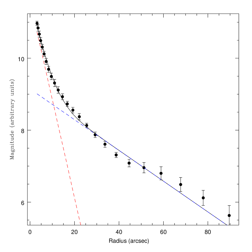
Figure 1: Azimuthally averaged radial surface brightness profile of NGC 2985 ($I$-band). Both the disc and the bulge component have been fitted with an exponential profile. The solid line is the sum of the two components.

We have applied the analysis described above to the Sab galaxy NGC 2985. It is a typical multi-armed spiral with an inclination of 36^∘ (Grosbol, 1985). Its distance, using an Hubble constant of 75, is 18 Mpc and the amplitude of the inclination corrected HI rotation curve is about 250 km/s (WHISP database), see table 1.

Table 1: Parameters of NGC 2985

Hubble Type	Sab
Inclination	36∘
Distance	18 Mpc
Max. rotational velocity	$\sim 250$ km/s
$M_{B}$	-21.10
Disc scale length	30” in $I$

3.1 Spectroscopy

Longslit absorption line spectra along the major axis (3.5 hours integration) and the minor axis (4 hours) of NGC 2985 were obtained with the ISIS spectrograph on the William Herschel Telescope in the first week of January 1997. These spectra were centered around the Mg b feature near 5200 Å. Calibrating arc lamp exposures were taken every 30 minutes. The dispersion per pixel is $\sim 0.4$ Å.

The longslit spectra were reduced to log-wavelength bins in the standard way, using IRAF packages. Adjacent spectra were averaged to obtain a signal-to-noise ratio of at least 25 per bin, and the absorption-line profiles of these co-added spectra were analysed. Velocity dispersions and radial velocities have been extracted from the absorption-line profiles using the traditional Gauss-fitting method after we had first established that the profiles are indeed close to having Gaussian shape. The observed spectra are compared with a template spectrum (HD107288, type K0III) convolved with a Gaussian. The Gaussian that best fits the data in a least square sense then yields the stellar radial velocities and the stellar velocity dispersions.

The derived velocity dispersions along the major axis are significantly better behaved (larger extent and less erratic behaviour) on the redshifted side of the centre than on the blueshifted side. This behaviour was also observed with the software of van der Marel (1994). It is even apparent in the kinematic data of Heraudeau et al (1999). We have therefore decided to only use the redshifted side of the major axis in the subsequent analysis. Hence we have only half as many data points on the major axis as we have on the minor axis, which looks regular on both sides of the centre. Around 20 arcsec from the nucleus there is some indication of a break in the profiles. Beyond this radius the velocity dispersion profiles flatten, suggesting that the disc component starts dominating the velocity dispersions.

The spectral range of the longslit absorption spectra also included the 5007 Å emission line. Fitting the mean of the emission line in each co-added spectrum gives us a direct measure of the circular velocity.

3.2 Photometry

The extent of the bulge can be assessed from a bulge-disc decomposition performed on a WHT $I$ band image obtained from the ING archive. Ellipses were fitted to the isophotes and an azimuthally averaged luminosity profile was extracted. The bulge component and the disc component of this profile were then simultaneously fitted assuming an exponential distribution for the disc component and either an exponential profile, Fig. 1, (Andredakis & Sanders, 1994) or a De Vaucouleurs profile for the bulge.

Using a De Vaucouleurs profile gives a slightly better $\chi^{2}$ value than using an exponential profile. The latter, however, is mathematically more sound since its derivative does not go to zero at the origin and it is physically more attractive because a De Vaucouleurs profile will at some (large) radius dominate the total light distribution again. With a double exponential distribution the bulge is significantly smaller than with an exponential disc and a De Vaucouleurs bulge. However, even in the latter case the disc dominates beyond a radius of 20 arcsec (but then only by a factor of a few).

Taking the average of the two different fitting procedures to represent the true disc scale length we derive an exponential disc scale length in the $I$ band of 30 $\pm$ 4 arcsec, close to the literature value of 35 arcsec (Grosbol, 1985).

4 Analysis

Table 2: Best-fit parameters and their corresponding one-sigma errors obtained from a brute force calculation. The errors in brackets are obtained from bootstrapping the data.

Parameter	Best-fit
$\sigma_{R,0}({\,\rm km\,s^{-1}})$	149 $\pm$ 12 (15)
$a$ (arcsec)	73 $\pm$ 9 (15)
$\sigma_{z,0}({\,\rm km\,s^{-1}})$	127 $\pm$ 10 (15)
$V_{0}({\,\rm km\,s^{-1}})$	136 $\pm$ 14 (28)
$\alpha$	0.18 $\pm$ 0.03 (0.07)

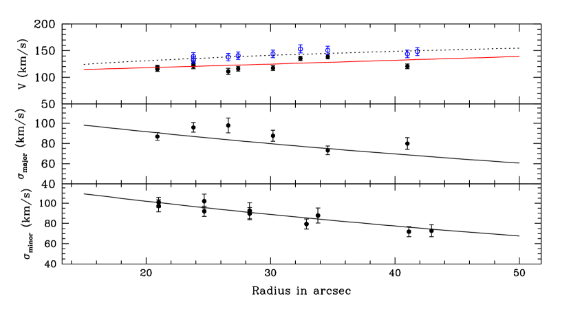
Figure 2: The best-fitting model distributions (solid lines for the stellar kinematics and a dotted line for the emission line kinematics) and the line-of-sight velocity data. Within 20 arcsec the bulge dominates the total light distribution. This region has therefore been excluded in the analysis. The open circles in the upper panel are measurements of the circular velocity determined from the emission line at 5007 Å while the filled circles measure the stellar rotation derived from the absorption lines.

The projected model distributions of section 2 were fitted simultaneously to the observables. However, unlike in Paper 1 we were unable to apply the non-linear fitting (Press et al. 1992) routines successfully, probably because the present data set is noisier and contains fewer data points. Fitting is therefore accomplished using a combination of a simulated annealing (a.k.a. biased random walk, Rix & White 1992) method and the downhill simplex method (Press et al. 1992). Since the number of data points is rather small we have included the emission line data directly into the fitting procedure. This allowed us to better constrain the model distributions although it also meant that we had to sacrifice the consistency check on the result.

Error estimates were obtained numerically since the minimisation of a function does not provide direct estimates of the uncertainties involved. One-sigma errors have been estimated from a brute force calculation. In this procedure we calculated $\chi^{2}$ values by varying all five fitting parameters in a broad range around their best-fit values (i.e. $\chi^{2}$ is sampled on a five-dimensional grid). One-sigma errors correspond to an increase of unity in $\chi^{2}$ over its best-fit value. The projection of the grid inclosure where $\Delta\chi^{2}=1$ onto the principal axes determines the one-sigma uncertainty in each individual parameter. A two dimensional projection of this grid is shown in Fig. 3. Here the grid is projected onto the plane spanned by the radial and vertical velocity dispersion axes. The distribution of points, ‘the error cloud’, not only yields the one-sigma errors but it also provides a measure of the covariance between the two parameters.

The confidence intervals have also been estimated from a Monte-Carlo study of a large number of new data sets, with each new data set drawn randomly from the original data set. This bootstrapping procedure resulted in slightly larger error-bars but did not change the numerical values of the parameters suggesting that the brute force calculation is probably a bit to restrictive in its estimate of the uncertainties. For the two parameters that we are most interested in, $\sigma_{R}$ and $\sigma_{z}$, the difference appears to be at a minimum anyway.

The obtained best-fit parameters are listed in table 2 and the corresponding model distributions are together with the data presented in Fig.2. The associated $\chi^{2}$ value of 50, however, is a bit higher than what is formally required by chi-square fitting. But the scatter of the data points around the best-fit models, especially along the major axis velocity dispersion is rather large and the large value of $\chi^{2}$ can probably be attributed to that. It even appears that the best-fit profile along the major axis actually lies too low given the data points. Along this axis the observed dispersions are a combination of the tangential and the vertical velocity dispersion components while the minor axis measures the radial and vertical components. Implying that the dispersions along the minor axis should be higher than along the major axis if the components are distributed in the canonical way, $\sigma_{R}>\sigma_{\phi}>\sigma_{z}$.

However, the difference between the circular velocity and the stellar rotation speed (top panel of Fig. 2) is roughly proportional to the radial velocity dispersion, see equation 4. A higher best-fit major axis profile therefore also implies a smaller difference between the circular velocity and the rotational velocity, which is certainly not warranted by this data set.

The best-fit kinematical scale length parameter, $a$, is about twice as large as the photometrical scale length. A result predicted by the local isothermal approximation of stellar discs (e.g. van der Kruit & Freeman, 1986).

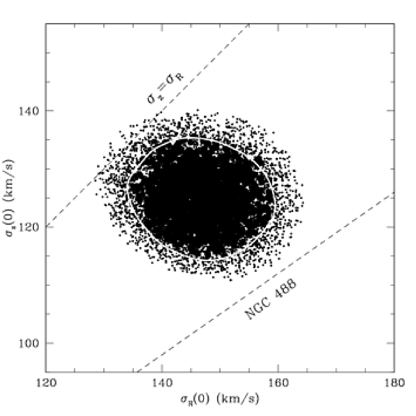
Figure 3: Distribution of the allowed range of values of the extrapolated central radial and vertical velicity dispersions. Small dots are random choices of the model paramaters (projected onto $\sigma_{R}(0)$, $\sigma_{z}(0)$) which are consistent with the data at the 2-$\sigma$ level, large dots are consistent at 1-$\sigma$. The white contour delineates the 1-$\sigma$ region. The upper dashed line indicates an isotropic $\sigma_{z}=\sigma_{R}$ velocity ellipsoid. The results obtained for NGC488 (Paper 1) are also indicated.

5 Discussion

The results derived in the previous section imply a ratio of the velocity ellipsoid of $\sigma_{z}/\sigma_{R}$ = 0.85 $\pm$ 0.1. The one-sigma error includes the covariance – evident from the fact that the distribution of points in Fig. 3 is not completely circular – between the two parameters. With the error estimates obtained from bootstrapping the ratio becomes 0.85 $\pm$ 0.13.

All the one-sigma points in Fig. 3 are located below the line $\sigma_{z}=\sigma_{R}$. Indeed, according to the generic picture of the gradual heating of stellar discs (Jenkins & Binney, 1990) the ratio $\sigma_{z}/\sigma_{R}$ – starting from an isotropic distribution of velocity dispersions – will become smaller than one given enough time. If only giant molecular clouds are responsible for heating this ratio will approach 0.75 and, if spiral structure also contributes to the disc heating the ratio will be lower. The derived ratio is therefore just consistent with the picture where disc heating is dominated by giant molecular clouds.

5.1 Comparison to other galaxies

Figure 4: Observed velocity ellipsoid ratios as a function of morphological RC3 type. The observed ratios in both NGC 2985 and NGC 488 are average values at one disk scale length while the value derived for the Galaxy is obtained at two disk scale lengths. The horizontal error bars reflect the uncertainty associated with classifying galaxies.

The obtained velocity ellipsoid axis ratio is a little higher but comparable to the value found for NGC 488 ($0.70\pm 0.19$). The slightly rounder velocity ellipsoid found in NGC 2985 may reflect a genuine difference in the internal heating mechanisms. Since both galaxies are multi-armed type spiral galaxies but the Sab galaxy NGC 2985 is of slightly earlier type than NGC 488, which is an Sb galaxy.

However, in both galaxies the axis ratios (average values around one disc scale length) are somewhat higher than in the solar neighbourhood (at about two disc scale lengths) where the most accurate measurements using the Hipparcos data indicate a ratio of 0.53 $\pm$ 0.07 (Dehnen & Binney 1998).

This behaviour is again consistent with the predictions of simple disc heating mechanisms since our own Galaxy is of type Sbc and therefore has a higher contribution from heating by spiral structure resulting in a flatter velocity ellipsoid.

This effect is illustrated in Fig. 4. The observed trend may be slightly fortuitous given the large error-bars on each point. However, photometric observations of edge-on galaxies (van der Kruit and de Grijs, 1999 and references therein) indicate a similar trend, i.e. late type spiral galaxies are more flattened than early type spiral galaxies.

A larger sample is clearly needed to clarify the significance of this trend. The relevant measurements for a single galaxy typically require one night on a 4m class telescope. Doubling or tripling the sample size can thus be done in a relative short time span and should unequivocally establish the validity of the current disc heating theories.

References

- [1] Andredakis Y.C., Sanders R.H., 1994, MNRAS, 267, 283
- [2] Binney J., Tremaine S., 1987 Galactic Dynamics. Princeton University Press, Princeton
- [3] Dehnen W., Binney J., 1998, MNRAS, 298, 387
- [4] de Vaucouleurs G., de Vaucouleurs A., Corwin H.G., Buta R.J. et al, 1991, Third Reference Catalog of Bright Galaxies. Springer Verlag, New York (RC3)
- [5] Gerssen J., Kuijken K., Merrifield M.R., 1997, MNRAS, 288, 618 (Paper 1)
- [6] Grosbol P.J., 1985 A&AS, 60, 261
- [7] Heraudeau Ph., Simien F., Maubon G., Prugniel Ph., 1999, A&ASS, 136, 509
- [8] Jenkins A., 1992, MNRAS, 257, 620
- [9] Jenkins A., Binney J., 1990, MNRAS, 245, 305
- [10] Kuijken K., Tremaine S., 1991 in Dynamics of Disc Galaxies. Götenborg Univ. and Chalmers Univ. of Technology, Götenborg, Sweden, p. 71
- [11] Press W.H., Teukolsky S.A., Vetterling W.T., Flannery B.P., 1992, Numerical Recipes. Cambridge University Press, Cambridge
- [12] Rix H-W., White S.D.M., 1992, MNRAS, 254, 389
- [13] Schwarzschild K., 1907 in Götingen Nachr., p. 614
- [14] Sellwood J.A., Nelson R.W., Tremaine S., 1998, ApJ, 506, 590
- [15] Shu F. H., 1969, ApJ, 158, 505
- [16] van der Kruit P.C., Freeman K.C., 1986, ApJ, 303, 556
- [17] van der Kruit P.C., de Grijs R., 1999 A&A, in press
- [18] van der Marel R.P., 1994, MNRAS, 270, 271