The Enrichment History of the Intergalactic Medium -
Measuring the C IV/H I Ratio in the Ly$\alpha$ Forest .

Abstract

We have obtained an exceptionally high S/N, high resolution spectrum of the gravitationally lensed quasar Q1422+231. A total of 34 C IV systems are identified, several of which had not been seen in previous spectra. Voigt profiles are fitted to these C IV systems and to the entire Ly$\alpha$ forest in order to determine column densities, $b$-values and redshifts for each absorption component. The column density distribution for C IV is found to be a power law with index $\alpha=1.44\pm 0.05$, down to at least log $N$(C IV) = 12.3. We use simulations to estimate the incompleteness correction and find that there is in fact no evidence for flattening of the power law down to log $N$(C IV) = 11.7 – a factor of ten lower than previous measurements. In order to determine whether the C IV enrichment extends to even lower column density H I clouds, we utilize two analysis techniques to probe the low column density regime in the Ly$\alpha$ forest. Firstly, a composite stacked spectrum is produced by combining the data for Q1422+231 and another bright QSO, APM 08279+5255. The S/N of the stacked spectrum is 1250 and yet no resultant C IV absorption is detected. We discuss the various problems that affect the stacking technique and focus in particular on a random velocity offset between H I and its associated C IV which we measure to have a dispersion of $\sigma_{v}$ = 17 km s^-1. It is concluded that, in our data, this offset results in an underestimate of the amount of C IV present by a factor of about two and this technique is therefore not sufficiently sensitive to probe the low column density Ly$\alpha$ clouds to meaningful metallicities. Secondly, we use measurements of individual pixel optical depths of Ly$\alpha$ and corresponding C IV lines. We compare the results obtained from this optical depth method with analyses of simulated spectra enriched with varying C IV enrichment recipes. From these simulations, we conclude that more C IV than is currently directly detected in Q1422+231 is required to reproduce the optical depths determined from the data, consistent with the conclusions drawn from consideration of the power law distribution.

1. Introduction

Our understanding of the intergalactic medium (IGM) has undergone a paradigm shift in recent years, largely as a result of powerful hydrodynamical simulations. When the Ly$\alpha$ forest was first observed in the late 1960s, the rich field of H I absorption blueward of the QSO’s Ly$\alpha$ emission was interpreted as the detection of discrete intergalactic clouds (e.g. Lynds & Stockton 1966; Lynds 1971; Sargent et al. 1980). In order to understand the existence of such isolated absorbers, various theories of cloud confinement, including self-gravity (Melott 1980), cold dark matter minihaloes (Rees 1986) and the presence of an inter-cloud medium (e.g. Sargent et al. 1980; Ostriker & Ikeuchi 1983) were proposed. However, the advent of hydrodynamical simulations, which model the growth of structure in the high redshift universe, provided a significant revision to our picture of the IGM (see the recent review by Efstathiou, Schaye and Theuns 2000). It has been found that in the presence of a UV ionizing background, the ‘bottom-up’ hierarchy of structure formation knitted a complex, but smoothly fluctuating ‘cosmic web’ in the IGM (e.g. Cen et al. 1994; Hernquist et al. 1996; Bi & Davidsen 1997). The absorption in the Ly$\alpha$ forest is caused not by individual, confined clouds, but by a gradually varying density field characterized by overdense sheets and filaments and extensive, underdense voids. The advance in theoretical simulations has been matched by increasingly high quality data, as comprehensively reviewed by Rauch (1998). One of the major discoveries concerning the IGM has been the identification of metal absorption lines associated with many of the Ly$\alpha$ forest clouds (Cowie et al. 1995; Tytler et al. 1995). Thus, whilst the Ly$\alpha$ forest was once thought to be chemically pristine, it has now been well-established that a large fraction of the high column density Ly$\alpha$ clouds ($N$(H I) $>$ 14.5), associated with collapsing, over-dense structures, contain metals (most notably C IV) – the signature of enrichment by the products of stellar nucleosynthesis (Songaila & Cowie 1996).

The presence of metals in the Ly$\alpha$ forest may be reasonably explained either by in-situ enrichment (local star formation in the H I cloud itself or in a nearby galaxy) or by early pre-enrichment by a high redshift episode of Population III stars. Whilst the effects of supernova feedback are still not fully understood and therefore the spatial extent of wind-driven ejecta is poorly constrained, enrichment by galactic winds and superbubbles is unlikely to be an efficient way to distribute metals over distances large in comparison with the mean separation between galaxies (MacLow & Ferrara 1999). Instead, models have appealed to larger scale processes such as merging and turbulent diffusion as the dominant mixing mechanisms (Gnedin & Ostriker 1997; Gnedin 1998; Ferrara, Pettini & Shchekinov 2000). Such processes would take time to smooth out the metallicity of the IGM so that at $z\sim 3$ the metal enrichment is still expected to be very patchy. Whilst the deep potential wells of galaxies inhibit efficient, widespread distribution of metals far from their sites of formations, small regions of star formation at high redshift may be able to eject their nucleosynthetic products for more homogeneous mixing (e.g. Nath & Trentham 1997 and references therein). An episode of Population III star formation may therefore have spread metals far from their sites of formation, seeding ‘sterile’ regions of the IGM with metals (Ostriker & Gnedin 1996). Clearly, distinguishing between in-situ and Pop III scenarios has important implications for understanding not only the first generation of stars, but also the mechanisms by which metals are mixed and distributed from their stellar birthplaces.

Several papers (Cowie & Songaila 1998; Lu et al. 1998; Ellison et al. 1999a, hereafter Paper I) have addressed this question by attempting to probe the low density regions of the IGM where the difference in metallicity predicted by in-situ and Pop III enrichment may be most marked. The detection of C IV $\lambda\lambda$1548,1550 associated with low column density Ly$\alpha$ clouds (log $N$(H I) $<$ 14.0) is observationally challenging, even with the capabilities of Keck, due to the extreme weakness of the metal lines. Analysis techniques have therefore been developed to effectively enhance the sensitivity of the data beyond the normal equivalent width limits of the spectra. Two in particular have received recent attention, namely the production of a stacked C IV spectrum (Lu et al. 1998) and the use of individual pixel optical depths of Ly $\alpha$ and C IV (Cowie & Songaila 1998). In Paper I we attempted to reconcile the apparently conflicting results obtained from these two techniques with an analysis of a very high signal-to-noise ratio (S/N) spectrum of the ultra-luminous BAL quasar APM 08279+5255. Rigorous testing of the analysis procedures revealed that both methods suffered from hitherto unrecognised limitations and it was concluded that the question of whether or not the low density regions of the IGM have been enriched remains unanswered.

In order to probe deeper into the low density IGM, we have obtained an exceptionally high S/N spectrum of the well-known lensed QSO, Q1422+231, using the HIRES instrument (Vogt 1994) on the KeckI telescope. Although this QSO has been well studied in the past (e.g. Songaila & Cowie 1996; Songaila 1998), we have roughly doubled the exposure time of earlier spectra, allowing us to probe the metallicity of the Ly$\alpha$ forest to more sensitive levels than has previously been achieved. The spectrum is much better suited to the present work than the the much more complex BAL quasar APM 08279+5255 (Ellison et al. 1999a). We present a careful and extensive analysis of the C IV systems in order to determine the extent of metal enrichment in the IGM. This paper is organised as follows. In §2 we describe the observations, the data reduction procedures and the Voigt profile fitting process used to determine column densities. We briefly discuss in §3 the suitability of Q1422+231 for this work and define the redshift interval over which we will perform the analysis. In §4, we determine the column densities of the 34 detected C IV absorption systems in the spectrum and investigate the column density distribution of these absorbers. Finally, we critically assess the two methods of analysis, described in sections 5 and 6, which have been developed to probe low column density Ly$\alpha$ clouds to very sensitive levels. We utilize a suite of simulation techniques to fully test these methods and quantify the potential inaccuracies in our analysis.

We adopt $\Omega_{M}$ = 1.0 throughout.

2. Data Acquisition and Reduction

Observations of Q1422+231 were made with the HIRES spectrograph (Vogt 1994) on the KeckI telescope in February 1999, using the $1.14\times 7$ arcsec slit. The resultant resolution is $R=37,000$. Individual exposure times varied between 30 min and 40 min, for a total exposure of 630 min in two (overlapping) grating settings to provide total wavelength coverage between the quasar’s Ly$\alpha$ and C IV emission lines. The data were reduced as described in Songaila (1998) and added to the spectrum of Q1422+231 obtained under similar conditions by Songaila and Cowie (1996). The total integration time for the two datasets is 1130 minutes and has a S/N of 200 – 300 redward of the QSO’s Ly$\alpha$ emission, a quality superior to all previously published data.

After extraction and sky subtraction, we noted that the cores of the saturated absorption lines contain a very small systematic residual flux. This error in the zero level is possibly due to light from a foreground source or a small underestimate of the background sky. The correction required to bring the line cores to zero was found to vary slightly with wavelength, ranging from 0.8% for the bluest absorption lines ($\lambda<4850$ Å) to 0.2% at $\lambda\sim 5500$ Å. No correction could be estimated redward of the QSO’s Ly$\alpha$ emission since the absence of saturated lines gave us no basis for estimating the adjustment required. However, since the correction factor required appears to diminish with increasing wavelength and is already very small at 5500 Å, and given that such an adjustment will make little difference to the relatively weak C IV lines studied in the red, we consider any residual eror to be unimportant for the analysis presented here.

The continuum fit was achieved using the STARLINK package DIPSO with a cubic spline polynomial applied to windows of spectrum judged to be free from absorption. Voigt profiles were fitted to the entire normalized Ly$\alpha$ forest using VPFIT (Webb 1987) to decompose the complex absorption into individual components defined by a column density ($N$(H I)), a $b$-value (Doppler width) and a redshift. This task, though time consuming, is an important feature of our analysis since synthetic spectra can be simulated based on the line list of Voigt profile parameters. For example, additional C IV associated with the fitted H I can be included to these synthetic spectra according to any desired enrichment recipe. As will be discussed later in this paper, this is an essential step for testing the analysis techniques used here.

3. Q1422+231 – Suitability and Sample Definition

Q1422+231 ($z_{em}=3.625$) is a well-studied quasar and actually consists of four closely spaced lensed images with separations of 0.5 – 1.3 arcsec; the lensing galaxy is at $z_{lens}$= 0.34 (Patnaik et al. 1992; Kundic et al 1997; Tonry 1998). Gravitational lenses enhance the emission from high redshift QSOs making them more powerful probes of the intergalactic and interstellar medium, but obviously the sight lines will sample different spatial regions of the intervening material. Its redshift and luminosity (V=16.5) have made Q1422+231 an ideal candidate with which to probe intervening material through closely spaced sightlines (Petry et al. 1998; Rauch et al. 1999). The observations reported here are of the closely spaced A and B components. In our observations the sightlines are unresolved. It is well established that multiple lines of sight through quasar pairs separated by several arcsecs show coherence between Ly$\alpha$ clouds on scales $>$ 100 kpc (e.g. Bechtold et al. 1994; Dinshaw et al. 1997). This is consistent with the scenario that has emerged from hydrodynamical simulations that portrays structure in the IGM not as discrete localized clouds but as a smoothly fluctuating medium. For metal line systems, whilst there may be slight differences in the individual components that constitute C IV complexes, Rauch et al. (1998) have shown that the total system column density remains largely unchanged over $\sim$ 10 kpc. The small linear separations probed by Q1422+231 ($<0.14$ kpc h^-1 for the C IV systems in the $z$ range considered here) are therefore unlikely to give rise to by line of sight differences so large as to compromise our column density determinations.

In order to avoid confusion between Ly$\alpha$ and higher order Lyman lines, we restrict our analysis of the Ly$\alpha$ forest in Q1422+231 to the interval 4740 $<\lambda$(Ly$\alpha$)$<5520$ Å which corresponds to a redshift range of 2.90 $<z_{abs}<$ 3.54. The lower limit of this interval is determined by the onset of Ly$\beta$ absorption and the upper limit is enforced in order to avoid effects due to quasar proximity (e.g. Lu, Wolfe & Turnshek 1991) and corresponds to a velocity separation of $\sim 5500$ km s^-1 relative to the emission redshift, $z_{em}$ = 3.625. In order to improve the statistics and S/N of stacked data (§5), we have, in some of the work presented here, included the spectrum of APM 08279+5255, recently analysed in Paper I. APM 08279+5255 is an ultra-luminous Broad Absorption Line (BAL) quasar with a systemic redshift $z_{em}$ = 3.911 and a broad band magnitude R = 15.2. The data obtained for this quasar (as presented in Paper I) are also of excellent quality, though the broad absorption line makes some portions of the spectrum less ideal for this problem than the spectrum of Q1422+231, and taken together with Q1422+231 they represent a premium data set for this work. The wavelength region used for APM 08279+5255 is 4995 $<\lambda$(Ly$\alpha$)$<5720$ Å (3.11 $<z_{abs}<$ 3.70) which in addition to the selection criteria applied to Q1422+231, takes into account the BAL nature of this quasar. Finally, a region contaminated by atmospheric absorption from 6865 $<\lambda$(C IV) $<$ 6940 Å (corresponding to $3.43<z<3.48$ for C IV) was excluded in both spectra.

4. Detected C IV Systems

Q1422+231 has been the target of several observing campaigns over the years, which have resulted in spectra of various S/N ratios. Whilst the primary motivation for obtaining such a high S/N spectrum was our scientific goal of probing the low column density Ly$\alpha$ forest, continued focus on this target has produced important results for IGM enrichment on a range of column density scales. In this section we present all of the detected C IV systems within the redshift range defined in §3, several of which have not been detected in previous spectra and we show that the power law column density distribution established for strong absorbers with $N$(C IV)$>$ 12.75 (Songaila 1997) continues to significantly lower column densities.

We detect 34 C IV systems within our defined wavelength interval, 29 of which are associated with saturated Ly$\alpha$ clouds (log $N$(H I) $\mathrel{\mathchoice{\vbox{\offinterlineskip\halign{\hfil$\displaystyle#$\hfil\cr>\cr\sim\cr}}}{\vbox{\offinterlineskip\halign{\hfil$\textstyle#$\hfil\cr>\cr\sim\cr}}}{\vbox{\offinterlineskip\halign{\hfil$\scriptstyle#$\hfil\cr>\cr\sim\cr}}}{\vbox{\offinterlineskip\halign{\hfil$\scriptscriptstyle#$\hfil\cr>\cr\sim\cr}}}}$ 14.5). These systems exhibit a wide variety of column densities and complexity (i.e. number of components) as can be seen in Figure 1. The column densities, $b$-values and redshifts determined for each C IV component using the Voigt profile fitting program VPFIT, are presented in Table 1. Examples of C IV systems detected in our spectrum which have not been observed in other published spectra (Songaila & Cowie 1996; Songaila 1998) are the weak systems at $z_{abs}=3.276,3.317$ and 3.518 (C24, C25 and C33 in Figure 1).

4.1. Column Density Distribution of C IV Systems

Previous studies of C IV absorbers in a variety of quasar sightlines has established a power law column density distribution (with index $\alpha\sim 1.5$, see eqn. 1) complete down to log $N$(C IV) $\simeq$ 12.75 at $z>3$ and 12.25 at $z<3$.(Songaila 1997). The column density distribution function is defined as

$$f(N)dN=BN^{-\alpha}dN$$ (1)

where, $f(N)$ is the number of systems per column density interval per unit redshift path. The redshift path (used instead of $z$ in order to account for co-moving distances) is given by $X(z)=\frac{3}{2}[(1+z)^{\frac{3}{2}}-1]$ for our adopted cosmology. An important question is how much of the iceberg has been exposed? To what limit does this power law distribution continue? As spectral data have improved, early determinations of the column density distribution of C IV absorbers have been shown to be incomplete at low column densities (compare for example Petitjean & Bergeron 1994 and Songaila 1997). The superb quality of this single spectrum can address whether the established power law continues to lower $N$(C IV), in which case the apparent fall-off towards low $N$(C IV) seen previously is due to incompleteness, or whether there is a real turnover in number density. In Figure 4 we show the column density distribution of C IV derived from the systems in Q1422+231, assumed to be a power law of the form of eqn. 1. A maximum likelihood fit to the data (binned in Figure 4 for display purposes only) gives a power law index of $\alpha=1.44\pm 0.05$, consistent with other recent estimates. This high quality spectrum, however, clearly uncovers more of the ‘iceberg’ than previous studies and the power law continues down to log $N$(C IV) $\sim$ 12.3 (Figure 4, solid points). Below this column density, $f(N)$ shows an apparent departure from the power law which may be due to incompleteness or alternatively reflect a real turnover in the $N$(C IV) distribution. The formal 5$\sigma$ detection limit for C IV in our spectrum is log $N$(C IV) = 11.6, for the median $b$-value of the observed C IV absorption lines, $b_{median}=13$ km s^-1. This detection limit is for one C IV line and is based on the $\lambda$1548 Å doublet component. However, identification of a suspected C IV system is dependent on confirmation from the weaker C IV $\lambda$1550 Å line whose oscillator strength is only half of the $f$-value of the 1548 Å line. This effectively reduces our sensitivity for detecting C IV systems by a factor of two to a 5$\sigma$ detection limit of log $N$(C IV) = 11.9. Moreover, lines with $b$-values significantly larger than the median $b$=13 km s^-1, may not be detected. In order to estimate the incompleteness for systems with log $N$(C IV) $<$ 12.3 due to large $b$, 40 C IV doublets were simulated for the two bins in Figure 4 which show a departure from the established power law, i.e. $N$(C IV) = 12.05 and $N$(C IV) = 11.75. The $b$-value for each line was drawn at random from the real distribution of Doppler widths and noise was added at the appropriate level. Each simulated line was then inspected to assess whether it would have been identified in the original spectrum so that a correction factor could be determined to estimate incompleteness. For $N$(C IV) = 12.05 a correction factor of 2.4 was determined (17/40 test C IV systems detected in the incompleteness trial), with the largest $b$-value in the lines detected being 13 km s^-1. In the lowest column density bin, $N$(C IV) = 11.75 only 9 out of 40 C IV lines (with $b<$ 8 km s^-1) were identified, corresponding to a correction factor of 4.4. Clearly, these correction factors assume that the $b$-value distribution does not significantly change with decreasing C IV column density. The two data points adjusted for incompleteness are represented by open circles in Figure 4. Thus, it appears that the power law distribution of column densities continues down to at least log $N$(C IV) = 11.75.

4.2. Homogeneous or Variable Metallicity?

Recently, hydrodynamical simulations have been used to predict the expected scatter in individual C IV/H I ratios within strong Ly$\alpha$ absorbers for a fixed [C/H] (Hellsten et al. 1997; Rauch, Haehnelt & Steinmetz 1997, Davé et al. 1998). When compared with observations, these models show that the data are consistent with a mean IGM metallicity [C/H] = $-2.5$ with variations of up to a factor of 10 around this average value. In these models, the C IV systems associated with high column density Ly$\alpha$ clouds are dominated by metals from in-situ star formation, since simulations show that these metal enriched clouds are found within a few tens of kpc from collapsed, dense clumps at $z\sim 3$ (e.g. Haehnelt 1998 and references therein). We would then expect the metallicity of such clouds to be variable, being dependent on the local star formation history, and therefore the scatter amongst individual C IV/H I ratios at a given $N$(H I) to be larger than that predicted for a homogeneous [C/H].

We can calculate C IV/H I ratios for 19 systems in our spectrum of Q1422+231. Of the 34 detected C IV systems in the spectrum presented here, 29 are associated with saturated Ly$\alpha$ lines. Although it is not possible to determine accurate H I column densities from these lines alone, for 14 of the C IV systems higher order Lyman lines are both accessible and suitably uncontaminated by blends so that an accurate $N$(H I) can in fact be derived. In addition, 5 of the systems in Q1422+231 are associated with clouds with log $N$(H I) $<$ 14.5 which are not saturated so that the column densities can be determined from the Voigt profile fit of Ly$\alpha$ only. The C IV and H I column densities determined for these 19 systems are presented in Table 3.

Davé et al. (1998) have also extensively studied the C IV/H I ratios of Q1422+231, as determined from the spectrum of Songaila & Cowie (1996). They constructed a mock spectrum of Q1422+231 from hydrodynamic simulations for comparison with the data. Having both simulated and observed spectra at their disposal, they measured C IV/H I ratios in both datasets in a consistent manner (using the AutoVP Voigt profile fitter, Davé et al. 1997), and found that an intrinsic scatter of approximately 0.5 dex in metallicity is required to fit the data. However, the observed range of C IV/H I ratios is the result of many complex effects, which include not only spatial variations in the temperature-density relationship, but also, for example, fluctuations in the ionizing background. These complex effects have not yet been fully incorporated into models and therefore we should be mindful that the scatter in measured values of C IV/H I is an upper limit to the variations in [C/H] when compared with homogeneously enriched simulations with a uniform ionizing background.

Davé et al. (1998) also found that the most robust diagnostic for determining the mean carbon abundance in detected C IV systems is $\langle$log $N$(C IV)$\rangle$, although this statistic is clearly dependent on the sensitivity of the data. As a consistency check, we determine the $\langle$log $N$(C IV)$\rangle$ for those C IV systems identified in our spectrum of Q1422+231 whose column densities are above the detection limit of the Songaila & Cowie (1996) spectrum (estimated to be log $N$(C IV $>$ 12.0). We calculate $\langle$log $N$(C IV)$\rangle$ = 12.77 which compares well with the value of 12.72 determined by Davé et al. (1998), considering the errors associated with column density determinations of individual C IV systems. This demonstrates that the different line finding and fitting procedures used on different spectra reproduce the same answer, even when the same systems are observed with a higher S/N. For Voigt profile fitting, this is an important point to make in a process that is sometimes not clear-cut. It is also an illustration that the detection limit of the spectrum used by Davé et al. (1998) was well determined and did not suffer from serious incompleteness. Ideally, one would like to see how the mean [C/H] varies as we detect progressively weaker C IV systems. However, a simple extrapolation to lower column densities is not possible, since the relation between $\langle$log $N$(C IV)$\rangle$ and [C/H] presented in Davé et al. (1998) is tailored specifically for the detection limits of their data. In order to apply this technique to the full sample of C IV systems detected in the new Q1422+231 spectrum presented here, it would be necessary to re-create a model spectrum to match our data. However, we remind the reader that the caveats mentioned in relation to the scatter of C IV/H I are also applicable here, a fact of which one should be aware when comparing observational and simulated results and interpreting the conversion to metallicity.

We can summarise the results from this section with the following conclusions. By obtaining an ultra-high S/N spectrum of the $z=3.625$ quasar Q1422+231, we have detected 34 C IV absorption systems with 2.91 $<z_{abs}<$ 3.54. Some hitherto undetected weak C IV systems are reported whose column densities are consistent with the established $f(N)$ distribution showing that this power law ($\alpha=1.44\pm 0.05$) continues down to at least log $N$(C IV) = 11.75, a factor of 10 deeper than the previous determination at $z>3$ in Songaila (1997). By fitting down the Lyman series, we are able to determine accurate C IV/H I ratios for 19 of the identified systems, rather than relying on a statistical estimate of the median metallicity as has often been done. Davé et al. (1998) have previously determined that the scatter in C IV/H I in the Q1422+231 spectrum of Songaila & Cowie (1996) requires an intrinsic scatter in the [C/H] of a factor of $\sim$ 3. Finally, by considering only the C IV systems above the detection limit, we obtain the same $\langle$log $N$(C IV)$\rangle$ as Davé et al. (1998), a statistic used to infer that the mean [C/H] = $-2.5$. However, we stress that these simulations do not take into account the full complexity of the physical processes determining the C IV/H I ratio in the IGM so that both the mean [C/H] and its scatter may change with future more detailed work.

5. Stacking

As discussed in previous sections, the C IV/H I ratio in low $N$(H I) systems may hold the key to understanding metal enrichment mechanisms in the IGM. Since one of the major limitations in detecting weak C IV lines is S/N, stacking many sections of the spectrum is one way to circumvent this problem (e.g. Norris, Peterson & Hartwick 1983; Tytler et al. 1995).

In our application of this technique, we select Ly$\alpha$ lines with 13.5 $<$ log $N$(H I) $<$ 14.0 whose corresponding C IV spectrum shows no obvious metal lines or contamination from other absorption features. Each section is de-redshifted to the rest frame, re-binned to the dispersion of the lowest $z$ system, weighted according to its S/N, stacked and finally re-normalized. The optimal weighting used to co-add the C IV sections is given by

$$w_{j}=\frac{1/\sigma_{j}^{2}}{\sum_{j}1/\sigma_{j}^{2}}$$ (2)

where $\sigma_{j}^{2}$ is the variance of the data. To achieve maximum sensitivity, we use low column density H I lines from both the APM 08279+5255 and Q1422+231 spectra. Within the ranges defined in §3, a total of 67 low $N$(H I) lines were identified in the two QSO sightlines. The resulting composite spectrum has a S/N = 1250 and shows no absorption at the rest wavelength of C IV, $\lambda_{0}=1548.2$, as can be seen from the top panel of Figure 5.

In order to place a significance limit on this non-detection, a synthetic spectrum was created, re-producing the Ly$\alpha$ forest of the 2 quasars from the fitted H I line lists. C IV was included for H I lines with log $N$(H I) $<$ 14.5 assuming a fixed C IV/H I ratio and $b$(C IV) = $\frac{1}{2}b$(Ly$\alpha$) (representing a combination of thermal and bulk motion, as found in Paper I). Figure 5 shows the results of stacking synthetic spectra with log C IV/H I = $-3.1$. The resultant absorption in this stack has an equivalent width of 0.15 mÅ and represents a 4$\sigma$ feature which we therefore adopt as the detection limit for our stacked data. Several analyses (e.g. Songaila & Cowie 1996; Paper I) have determined the C IV/H I ratio in high column density Ly$\alpha$ clouds to be in the range from log C IV/H I = $-2.9$ to $-2.6$. The detection limit of the synthetic stack is almost factor of two lower than the metal-poor limit of this range, and thus it would appear to indicate a drop in the C IV/H I ratio at lower H I column densities. It must be understood, however, that this technique has several potential problems which may compromise its efficiency in detecting weak absorption features. We now discuss these problems in turn.

• In order to co-add each section, the data must be re-binned, usually to the dispersion of the lowest redshift system. This could smooth out a weak feature, although the scale of smoothing is very small compared with the width of the expected line so that this is not likely to be a major effect.

• Even for a fixed carbon abundance there will be a scatter in the values of C IV/H I (as discussed in the previous section). Therefore, if absorption is detected in the composite spectrum it will be averaged over a range of column densities that can not be recovered individually. Moreover, depending on the scatter of C IV/H I values, the absorption may be dominated by the strong tail end of this metallicity range. In fact, it is conceivable that residual absorption could be caused by only a few relatively strong lines, since this method relies on an average which is very sensitive to a non-Gaussian tail. Interpreting a residual signal in the composite spectrum is therefore not straightforward, although in the analysis presented here we find that there is no absorption in the stacked data and so we can determine a useful detection limit.

More serious problems for the present analysis are:

• The sensitivity of this method to errors in continuum fitting, anomalous pixels and other forms of contamination. The usual procedure is to visually inspect each section before adding it to the stack in order to ensure that it is ‘clean’. This will filter out major contamination by, for example, uncorrected cosmic ray events or absorption due to systems other than C IV. However, small errors in the continuum fit or deviant pixels could seriously compromise the efficiency of the stack. In addition, a re-normalization of the composite spectrum is usually required, since the small errors in the original continuum fit have now been compounded by stacking.

• Stacking the individual sections of spectrum in order to build up a signal is pivotal upon centering the absorption feature in the composite. If there is a significant error in the stack center, i.e. if an offset exists between the redshift of the parent Ly$\alpha$ line and its associated C IV complex, the composite signal would be smeared out. Depending on the magnitude of the offset, this effect may lead us to under-estimate the amount of absorbing material. This problem could be exacerbated by the afore-mentioned need for a re-normalization because it may be difficult, if not impossible, to distinguish a weak smeared signal from the compound continuum errors.

5.1. Redshift Offset Between C IV and Ly$\alpha$

In Paper I, we showed that there is indeed a random redshift offset ($\Delta z$) between the measured position of the Ly$\alpha$ and corresponding C IV lines. In that work it was found that the redshift offset had a distribution with $\sigma_{z}\sim$ 4 $\times 10^{-4}$ equivalent to a velocity difference of 27 km s^-1, although this statistic was based on a relatively small number of systems. The addition of a second quasar to the analysis has improved the statistics and for a total of 56 C IV systems in the two quasars we now determine a $\sigma_{z}$=2.6 $\times 10^{-4}$ ($\sigma_{v}\sim$17 km s^-1 for an average redshift of 3.45). This redshift offset was determined in two different ways. In both cases the redshift of the C IV was estimated by taking the centroid of the system since it is often complex, consisting of several blended components. For most of the corresponding Ly$\alpha$ lines, the absorption is well represented by a single component and so in the first instance the redshift of the H I cloud was obtained from the Voigt profile fit. For comparison, the redshift of Ly$\alpha$ was also determined using the same centroid method applied to the C IV systems and it was found that both determinations yielded almost identical results for the distribution of $\Delta z$, shown in Figure 6. Since it is the strongest component in each C IV complex that first emerges from the noise in the weak systems, this will be the feature enhanced by the stacking procedure. Therefore, we also investigated the distribution of offsets between the fitted $z$ of Ly$\alpha$ and the redshift of the deepest C IV trough and once again the value $\sigma_{v}\sim$ 17 km s^-1 was found.

We investigated how seriously the composite spectrum would be affected by this offset which effectively shifts the expected positions of the C IV lines by a random amount. Again, synthetic spectra were produced, this time including a redshift offset applied to the position of the C IV line with $\Delta z$ drawn at random from a Gaussian distribution with $\sigma_{z}$=2.6$\times 10^{-4}$. We find that in order to reproduce a 4$\sigma$ detection in the presence of a redshift offset, twice as much C IV must be included in the Ly$\alpha$ forest clouds, i.e. log (C IV/H I) = $-2.8$, see the bottom panel of Figure 5. This is consistent with the measured C IV/H I in log $N$(H I)$>$14.5 lines and is therefore not a sufficiently sensitive limit to establish whether the low column density Ly$\alpha$ clouds contain significantly less C IV that the stronger lines. We conclude that a factor of at least two improvement in sensitivity is required in order to show conclusively whether the low column density absorbers are more metal deficient than their high column density counterparts. Alternatively, it must be shown that the redshift offset in these lines is $\ll$ 17 km s^-1 and dilution of absorption from smearing the stack is unimportant.

The redshift offset in saturated lines could have two possible explanations, one physical and the other an observational artefact. There could be an intrinsic redshift difference between the C IV and Ly$\alpha$ absorbers, caused by, for example, ionization effects or outflows. An additional effect could be a redshift offset caused by the blending of strong Ly$\alpha$ lines which, when saturated, can not be distinguished into separate components. Two examples of this are shown in Figure 7. Plotted in velocity space are two examples of Ly$\alpha$ absorbers (black solid line) and corresponding C IV (dashed line). Both saturated (systems ‘b’ and ‘c’) and weak (systems ‘a’ and ‘d’) Ly$\alpha$ clouds are shown and in the top panel the Ly$\beta$ (in gray) is also included. The C IV system ‘c’ is associated with an apparently monolithic Ly$\alpha$ absorber centered at $v$ = 0 and exhibits a redshift offset of approximately 25 km s^-1. However, as seen from the Ly$\beta$ absorption, this system is made up of more than one component and the C IV clearly has a redshift that more closely matches the strongest of these. The unsaturated Ly$\alpha$ absorber associated with the C IV system ‘a’ does not break down into a multi-component system in Ly$\beta$ and the redshift offset is correspondingly small ($\Delta z<$ 1 km s^-1). However, there are other examples of C IV systems associated with weak Ly$\alpha$ that do show a significant offset, for example system ‘d’ in the lower panel of Figure 7. Unfortunately, higher order Lyman lines are not available for this particular case. We re-measured the redshift offset for each of the 19 C IV systems in Table 3 for which an accurate $N$(H I) had been obtained by tracing down the Lyman series. For 16 of these systems, the C IV appeared to be associated with a single H I component (i.e. not obviously blended), as seen from Ly$\beta$ and/or Ly$\gamma$. The offsets associated with the sub-cloud whose redshift most closely matches that of the C IV are shown in the lower panel of Figure 6. Given the small number of systems for which the Lyman series can be traced, at least to Ly$\beta$, the statistics of the offset distribution are not very meaningful. However, the scatter is now clearly smaller, although the high $N$(H I) Ly$\alpha$ lines at the top end of the column density distribution may still have several sub-components that are unresolved in our data and the offset may be further reduced if the Lyman series could be traced down to subsequent transitions.

5.2. An Improvement on the Stacking Method?

We investigated a possible solution to the problem of an unknown offset from the predicted position of C IV systems discussed above. The technique involves scanning for the maximum absorption around the predicted position of C IV absorption and re-centering the stack at this wavelength. In practice, each (de-redshifted) data section is scanned $\pm 2\sigma_{z}$ from the predicted C IV line center (i.e. for $\Delta z$ = 0) and the section re-centered on the pixel with the maximum optical depth ($\tau_{max}$) prior to stacking. Figure 8 shows an example of how this technique is clearly able to improve upon a direct stack in the presence of a $\Delta z$ for a synthetic spectrum containing lines with log C IV/H I =$-$2.0. It can be seen that without re-centering, whilst the overall level of the continuum is below unity for the ‘smeared’ stack, all profile information is lost. Such a broad depression may be mistaken for compound errors in the continuum level and lost in the subsequent renormalization of the stacked spectrum. Executing a re-center on the $\tau_{max}$ pixel before stacking recovers almost all of the original signal in this simulation, the characteristic line profile is prominent and will not be lost when the post-stacking continuum is re-fitted.

However, as one attempts to detect progressively weaker absorption, the likelihood of centering on a noise pixel becomes higher and this technique is no longer efficient. In order to determine whether a ‘re-center’ is a viable improvement to the stacking method, given the S/N of the data and the low column density of the targeted features, we performed a feasibility study in which test absorption lines were created over a range of C IV/H I ratios. The results of this study are shown in Figure 9 where we plot the distribution of $\sigma_{z}$ caused by line center misidentification (i.e. where $\tau_{max}$ is a noise feature rather than line trough) as a function of C IV/H I ratio. Clearly, when the $\sigma$ of the offset caused by trough misidentification exceeds the value of the intrinsic offset we are trying to overcome, this re-centering technique is no longer useful. However, these are conservative estimates for how well the centering would perform on real data, since we would expect some trough misidentification from contaminating (i.e. anything but C IV) lines in addition to the effects of noise investigated here. Since we need to determine whether the low column density Ly$\alpha$ lines have the same metallicity as their high $N$(H I) counterparts, we must ideally reach levels of sensitivity deeper than log C IV/H I=$-2.9$. Figure 9 shows that for log C IV/H I $<-$2.6, this technique no longer compensates adequately for the intrinsic offset and is therefore unable to improve the stacking technique in the search for weak lines. Smoothing the spectrum over several pixels before locating $\tau_{max}$ improves the pre-shifting slightly as shown by the gray squares in Figure 9. However, even with smoothing, this re-centering procedure can not compensate for a $\sigma_{z}$ = 2.6 $\times 10^{-4}$ below a log C IV/H I = $-2.75$.

In summary, by stacking together the C IV regions associated with low column density Ly$\alpha$ lines in Q1422+231 and APM 08279+5255, we have obtained a S/N = 1250 composite spectrum which shows no residual C IV absorption. Using simulated spectra we find that for log C IV/H I = $-3.1$ in the weak Ly$\alpha$ lines we would expect a 4$\sigma$ detection of the composite absorption. The shortcomings of this technique are discussed and we focus on an observed redshift offset between the position of Ly$\alpha$ and its associated C IV. The redshift offset determined from the detected C IV systems has a dispersion $\sigma_{z}$ = 2.6$\times 10^{-4}$ which corresponds to a $\sigma_{v}$ = 17 km s^-1. We have investigated how this offset would affect the stacking procedure by using simulated spectra and find that a $\sigma_{v}$ = 17 km s^-1 will reduce the sensitivity of this method by a factor of two and that a metallicity of log C IV/H I = $-2.8$ is now required to achieve a 4$\sigma$ detection. We are unable to know whether the same redshift offset persists in the low $N$(H I) clouds targeted by the stacking technique, but a large range of offsets are measured over the full column density range of detected C IV systems, so one must clearly take into account the possible repercussions when interpreting the stacked data.

6. Analysis of Optical Depths

A potentially more robust way of measuring weak absorption in high S/N spectra is to analyse the optical depths in each Ly$\alpha$ forest pixel and its corresponding C IV pixel (Cowie & Songaila 1998). This technique also has the advantage that by tracing down the Lyman series, one can determine the C IV/H I ratio in each pixel over a very large range of $\tau$(Ly$\alpha$). In Paper I we investigated the potential of this method with APM 08279+5255 and critically analysed its performance on synthetic spectra. Specifically, we investigated the effect of including a redshift offset and how the results depended on the $b$-value of C IV. We concluded that, despite the excellent quality of the spectrum, the results from the spectrum of APM 08279+5255 were inconclusive and could not determine whether the metallicity of the IGM is constant or diminished at low values of H I, because at the lowest values of $\tau$(Ly$\alpha$) both scenarios were consistent with the observations. The spectrum of Q1422+231 presented here not only has a significantly higher S/N than that of APM 08279+5255, but has many of its higher order Lyman lines accessible for analysis and considerably less contaminating absorption by, for example, Mg II systems (Ellison et al. 1999b). This spectrum therefore represents the best data yet obtained for this analysis of the low column density Ly$\alpha$ forest.

6.1. The Analysis Procedure

Briefly, the optical depth technique consists of stepping through the Ly$\alpha$ forest measuring $\tau$(Ly$\alpha$) for each pixel. The noise ($\sigma$) array is used to determine which pixels are included in the analysis via a series of optical depth criteria to account for effects such as saturation. Using the values in the noise arrays rather than fixing the rejection criteria provides maximum flexibility for this technique so that it can be readily applied to spectra of different S/N ratios.

For pixels with a residual flux ($F=e^{-\tau}$ for a normalised spectrum) $F<3\sigma$ above the zero level, we trace down the Lyman series since there is too little residual flux in these saturated pixels to determine an accurate optical depth from Ly$\alpha$ alone. However, the danger here is that higher order lines may be contaminated by lower redshift Ly$\alpha$. We therefore use $\tau$(Ly$\alpha$) = minimum($\tau$(Ly$n$)$f_{\rm{Ly\alpha}}\lambda_{\rm{Ly\alpha}}$ / $f_{\rm{Ly}n}\lambda_{\rm{Ly}n}$) over all observed higher order lines using the higher order pixel if $3\sigma<F$(Ly$n)<(1-3\sigma)$. This minimizes the effect of contamination and maximizes the number of usable pixels and range of $\tau$(Ly$\alpha$) which can be considered for analysis. If no $3\sigma<F$(Ly$n)<(1-3\sigma)$ pixels are found, then the pixel is discarded. The position of the associated C IV $\lambda\lambda$1548, 1550 lines are calculated and, again to avoid contamination, we use $\tau$(1548)= minimum($\tau(1548)$,$2\tau$(1550)) if the flux in the 1550 Å component $<1-3\sigma$, otherwise only $\tau$(1548) is considered. The C IV optical depths are then binned according to their corresponding $\tau$(Ly$\alpha$) and the median determined for each interval. Taking the median of a large number of pixel optical depths not only provides a statistical advantage over considering a relatively small number of lines (as for the stacking method), but also is much less susceptible to non-Gaussian effects. In order to estimate 1 $\sigma$ errors for the optical depth determinations, we used bootstrap re-sampling with 2Å sections of the Ly$\alpha$ forest and corresponding C IV, i.e. we drew $n$ random sections from the complete set of $n$ sections (in this case $n=361$) that comprise the original data, with replacement. This procedure was repeated 250 times and the 1$\sigma$ error was taken to be the dispersion of these 250 realizations.

6.2. Results

Figure 10 shows the results obtained for the optical depth analysis of Q1422+231. The shape of the optical depth distribution appears consistent with a constant level of C IV/H I (i.e. parallel to the dashed line) over optical depths from $\tau$(Ly$\alpha$) $\sim$ 100 down to $\sim$ 2 – 3, below which $\tau$(C IV) flattens off to an approximately constant value. Each of the low optical depth bins ($\tau$(Ly$\alpha$) $<$ 3) contains approximately 10% of the H I pixels. This percentage decreases with increasing $\tau$(Ly$\alpha$) with only approximately 2% of pixels in the $\tau$(Ly$\alpha$) = 10 bin. In addition, we determine optical depths in pixel pairs separated by the C IV$\lambda\lambda$1548, 1550 doublet ratio regardless of $\tau$(Ly$\alpha$) over the entire range considered for C IV absorption. This is done using the same method of doublet comparison as before to eliminate contamination. The median of this reference distribution is plotted in Figure 10 as a dotted line and represents the median absorption for an effectively random set of pixel pairs separated by C IV doublet ratio and will include the effects of noise and low level contamination expected to affect our results. This median optical depth is higher than the observed $\tau$(C IV) for all bins with $\tau$(Ly$\alpha$)$\;\buildrel<\over{\sim}\;$ 1. This is a significant result which indicates that the C IV absorption for these optical depths is less than that expected by selecting random pixel pairs. The key question here is whether the signal in the low optical depth H I pixels is due to C IV absorption in low density regions of the IGM or whether the flattening of the data is caused by some limiting factor in our analysis such as contamination or noise.

6.3. Testing the Results

As we saw in the previous section, thorough simulations of the analysis technique are vital for interpreting our results. Here, we have taken the Ly$\alpha$ forest directly from the data and artificially enriched it with C IV to test our methods and address several questions. In Paper I we explored the effect of $b$-values, redshift offset and noise on synthetic spectra in order to determine whether a break in the C IV/H I distribution could be distinguished from a constant ratio in the spectrum of APM 08279+5255. To review these findings and to give a visual impression of the optical depth analysis, we show the results of this technique on four synthetic spectra in Figure 11 and compare them with the results from Q1422+231 (solid points). The top panel (‘A’) of this figure shows the optical depth analysis of 2 spectra, one of which has a constant log C IV/H I = $-2.6$ in all Ly$\alpha$ lines (shown as a dotted line) and a second spectrum which has log C IV/H I = $-2.6$ only in log $N$(H I) $>$ 14.5 lines (dot-dashed line), with no noise added to either spectrum redward of Ly$\alpha$. The bottom panel shows the same spectra as panel ‘A’ except that noise has now been added to both spectra, based on the error array of the actual data (typically S/N = 200 redward of Ly$\alpha$). All four spectra use the real Ly$\alpha$ forest of Q1422+231 and have had C IV added to the synthetic spectrum based on the fitted H I linelist. In addition, all four synthetic spectra in Figure 11 have a $\Delta z$ = 2.6 $\times 10^{-4}$ and $b$(C IV) = $\frac{1}{2}b$(Ly$\alpha$). The dashed line indicates constant log C IV/H I = $-2.6$.

There are several points to note here. Firstly, in the absence of noise, there is a clear drop in $\tau$(C IV) below $\tau$(Ly$\alpha$) $\sim 3$ if no C IV is added in Ly$\alpha$ lines with log $N$(H I) $<$ 14.5. However, this steep decline is much less drastic when noise is included, and although $\tau$(C IV) shows a steady decrease down to $\tau$(Ly$\alpha$) $\sim$ 1, below this value it flattens off to an approximately constant value. The inclusion of noise also causes the same apparent flattening in the spectrum of constant C IV/H I, although the $\tau$(C IV) in this spectrum is consistently above the value measured for the dot-dashed line. There is also a small contribution to this flattening from line blending which changes the overall slope of the expected C IV/H I, an effect that is exacerbated for larger $b$(C IV). This shows that even in relatively high S/N spectra, distinguishing a break in the C IV/H I distribution is very difficult. Instead, as we shall see later in this section, one of the main uses of this method is to determine whether the optical depths measured with this technique can be adequately accounted for with the detected C IV systems or whether there must be significant amount of C IV still below our current detection limit. We also note that for large $\tau$(Ly$\alpha$) the measured $\tau$(C IV) is always less than expected from the dashed line, given the input ratio of C IV/H I. This is due to two effects. Firstly, since this technique considers $\tau$(Ly$\alpha$) as the minimum value obtained by tracing down the Lyman series when a line is saturated, if contamination is successfully removed we will tend to under-estimate $\tau$(Ly$\alpha$) at these optical depths due to noise (remember that the real Ly$\alpha$ forest is used in the simulated spectra so that this will be an effect even in panel ‘A’ of Figure 11). Secondly, the C IV that is included in the synthetic spectra is based on a linelist of fitted H I values which will probably not be accurate for saturated lines. These effects also account for the drop of $\tau$(C IV) at very large $\tau$(Ly$\alpha$) which contain $<$ 1% of the total H I pixels and are therefore very uncertain.

Clearly, the exact results of the optical depth analysis are sensitive to the combination of several factors including blending, $b$-values and noise, which we will discuss further later in this section. Therefore, rather than attempting to directly fit the observed distribution of optical depths in Q1422+231 we aim to determine whether the optical depths measured in the spectrum can be explained solely by the relatively strong C IV absorbers detected directly and presented in §4 or whether the results from this analysis are indicative of additional C IV. If the latter is true, are these metals in the low density IGM? We must also investigate whether our results can be explained in terms of contamination, noise or some other limiting factor in the data. Finally, we consider the effect of scatter and redshift offset ($\Delta z$), which have been found to compromise the efficiency of the stacking method.

Three synthetic spectra were produced with Ly$\alpha$ forest absorption taken directly from the data (i.e. not reconstructed from a linelist) and the 34 detected C IV systems re-produced from the Voigt profile parameters in Table 1. Spectrum ‘A’ has had no further metals added and therefore shows the results expected of an optical depth analysis if we had already uncovered all of the C IV in the spectrum. Spectra ‘B’ and ‘C’ have both been enriched with additional metals. In spectrum ‘B’, C IV is included in all strong (log $N$(H I) $>$ 14.5) lines with $N$(C IV) = 12.0, i.e. the detection limit for directly identifiable C IV systems. This spectrum therefore represents the maximum amount of C IV that could be ‘hidden’ in high column density Ly$\alpha$ lines. In addition to this ‘hidden’ C IV in strong H I lines and the fitted C IV in Table 1, spectrum ‘C’ has been enriched with a constant log C IV/H I = $-2.6$ in weak Ly$\alpha$ lines ($N$(H I) $<$ 14.5). The results from analysis of these three synthetic spectra are compared with the data in Figure 12. For all three spectra, we include noise taken from the $\sigma$ error array, a random redshift offset in the position of C IV ($\sigma_{z}=2.6\times 10^{-4}$) and take $b$(C IV) = $\frac{1}{2}$ $b$(Ly$\alpha$).

The conclusions that can be drawn from Figure 12 are as follows. First, there is clearly more C IV in the data than we have directly identified in §4, since the dotted line of the synthetic spectrum in the top panel is well below the solid line at all but the very highest $\tau$(Ly$\alpha$) points. For $\tau$(Ly$\alpha$) $\mathrel{\mathchoice{\vbox{\offinterlineskip\halign{\hfil$\displaystyle#$\hfil\cr>\cr\sim\cr}}}{\vbox{\offinterlineskip\halign{\hfil$\textstyle#$\hfil\cr>\cr\sim\cr}}}{\vbox{\offinterlineskip\halign{\hfil$\scriptstyle#$\hfil\cr>\cr\sim\cr}}}{\vbox{\offinterlineskip\halign{\hfil$\scriptscriptstyle#$\hfil\cr>\cr\sim\cr}}}}$ 3, the C IV optical depths can be recovered when additional metals are added into strong Ly$\alpha$ absorbers, but below our current detection limit (spectrum ‘B’). This supports the results of §4 where we determine that $f(N)$ is consistent with a power law distribution that continues down to log $N$(C IV) = 11.75, with no evidence for a turnover in column density distribution. However, adding C IV at the limit of our detection in log $N$(H I)$>$ 14.5 lines with no extra metals in weaker Ly$\alpha$ clouds can not reproduce the measured $\tau$(C IV) in $\tau$(Ly$\alpha$)$<$ 3 pixels. The results from spectrum ‘C’ in the bottom panel of Figure 12 which include log C IV/H I = $-2.6$ in weak Ly$\alpha$ lines show that the observed C IV optical depths in the low $\tau$(Ly$\alpha$) pixels are consistent with the presence of some metals in significantly lower column density H I clouds, although for $\tau$(Ly$\alpha$) $>$ 1 $\tau$(C IV) exceeds the observed value. From Figure 11 we have also seen that a constant log C IV/H I = $-2.6$ in all Ly$\alpha$ lines is a good approximation to the data. We stress here that these simulations are not an attempt to fit the observed distribution of optical depths, rather they are tests to determine whether the C IV systems in Table 1 can account for the measured absorption. If not, then the objective is to investigate in which H I column density regime additional metals could be added in order to achieve the observed quota.

The results from these simulations show that the analysis of optical depths in the spectrum of Q1422+231 is consistent with hitherto undetected C IV in both the strong and weak Ly$\alpha$ lines. Whilst the results from our determination of the column density distribution from detected C IV systems is consistent with a power law function $f(N)$ that continues down to at least log $N$(C IV) = 11.7, these optical depth results provide direct evidence that there are more metals lurking below our current detection limit.

We investigate the effect that contaminating lines may have on this result. The analysis may be affected not only by low level contamination from other metal lines such as Si IV or telluric absorption (strong absorbers will have been rejected by the C IV doublet strength comparison discussed in §6.1), but also effects due the non-uniformity of ionizing sources and noise/fluctuations in the continuum level due to fitting errors. This latter effect will cause fluctuations around the true continuum which will be important only if they are greater than the level of the noise. An additional (possibly systematic) error may be present if the low order polynomial fit to the continuum is consistently over or under-estimated. To test the continuum fit of the C IV regions, sections of the data redward of Ly$\alpha$ deemed to contain no obvious absorption were examined. From a total of $\sim$ 5000 pixels, a mean flux of 1.0002 and a median of 1.0001 were determined, vaules one order of magnitude lower than $\tau$(C IV) $\sim 10^{-3}$. It therefore seems unlikely that a systematic error in the continuum fit is the cause of the observed flattening of C IV optical depths seen in Figure 10. The distribution of noise pixels would also suggest that there is no significant effect from weak telluric lines. Errors in the continuum fit blueward of Ly$\alpha$ emission, however, are likely to be a more serious effect, firstly because selection of absorption-free zones is difficult and secondly because the S/N is lower (50 – 150). The result of continuum fitting errors in the forest in this analysis will be to classify pixels with small $\tau$(Ly$\alpha$) into the wrong optical depth bin. This will effectively associate C IV with the wrong $\tau$(Ly$\alpha$) and averaging out the metal absorption by this ‘mis-binning’ could explain the observed flattening of the measured optical depths. The effect of a small continuum error is therefore similar to the effect of noise, affecting only those pixels with optical depths smaller than the fitting error. We also find that including a large number of weak contaminating lines such as Si IV or Mg II could increase the measured $\tau$(C IV) at low $\tau$(Ly$\alpha$) to the constant level determined. However, whilst realistic column densities do have a small effect on the optical depth result, it is unlikely that weak contaminating lines account for all of the observed absorption.

As discussed previously, a scatter is expected in the observed C IV/H I values even if [C/H] and the ionizing background remain uniform. To investigate the importance of this effect, we simulated a ‘control’ spectrum by re-producing directly the Ly$\alpha$ forest of Q1422+231 and using $b$(C IV) = $\frac{1}{2}b$(Ly$\alpha$) and an input log C IV/H I = $-2.6$ with no scatter and no redshift offsets. For comparison, we then produced a second spectrum in the same way, but rather than adopting a constant C IV/H I, a Gaussian scatter was introduced with $\sigma$(C IV/H I) = $1\times 10^{-3}$. The comparison between the two simulated spectra is presented in Figure 13 where the ‘control’ spectrum is shown as open squares connected with a solid line and the spectrum containing a scatter of metallicities is shown as solid diamonds connected with a dotted line. The points have been offset from one another in the figure for clarity. The points at high $\tau$(Ly$\alpha$) are again very uncertain due to the reasons previously discussed with regards to Figure 11. The error bars are estimated using the same bootstrap technique as employed for the data. The results from the 2 spectra are entirely consistent with one another and indicate that a Gaussian scatter will therefore not affect the overall median of $\tau$(C IV). Whilst the extent and magnitude of the scatter in the distribution of C IV/H I values has not yet been fully investigated in simulations down to column densities below log $N$(H I) $\sim$ 14.0 – 13.5, this result should not be significantly affected unless the scatter becomes highly non-Gaussian at low $N$(H I). Also plotted in Figure 13 are the results of the optical depth analysis if a redshift offset is included in the position of the C IV line. As before, metals are added to all Ly$\alpha$ lines with a metallicity log C IV/H I = $-2.6$. There is no scatter in these values, but an offset in the position of C IV has been included, drawn at random from a Gaussian distribution with $\sigma_{z}=2.6\times 10^{-4}$ ($\sigma_{v}$ = 17 km s^-1). These points are also consistent with the control spectrum, so we can conclude from this simulation batch that neither scatter in the metallicity nor redshift offset will have a large effect on the outcome of our optical depth analysis.

Finally we note that more spectra are required in order to provide a representative analysis of the high redshift IGM, since our view of the enrichment of the Ly$\alpha$ forest probed with a single sightline is clearly blinkered. From the list of C IV systems in Table 1 it can be seen that these absorbers are not uniformly distributed in redshift. For example, splitting this spectrum in two by redshift produces vastly different optical depth distributions due to a relative dearth of C IV systems that spans over 300 Å in this spectrum in the range $3.13<z_{a}bs<3.33$. With more spectra, there is the possibility of not only developing a more representative study of these high redshift absorbers but also investigating the redshift evolution of C IV systems.

7. Conclusions

In this paper, we have addressed the enrichment history of the IGM by studying the Ly$\alpha$ forest and its associated C IV systems in a very high S/N ($\sim 200)$, high resolution ($\sim$ 8 km s^-1) spectrum of the well-known lensed quasar, Q1422+231 obtained with Keck/HIRES. The numerous C IV systems associated with high column density Ly$\alpha$ absorbers are fitted with Voigt profiles defined by a redshift, $b$-value and column density for each component line. We investigate the C IV column density distribution, $f(N)$, to very sensitive levels and detect several weak C IV systems which had not been previously identified in lower quality spectra of the same object. We determine a power law index $\alpha=1.44\pm 0.05$ which continues down to log $N$(C IV) = 12.2 before starting to turnover. By simulating synthetic absorption lines with $b$-values taken at random from the observed distribution, we estimate a correction factor to account for incompleteness and find that the corrected data points now indicate that the power law continues down to at least log $N$(C IV) = 11.75, a factor of ten more sensitive than previous measurements (e.g. Songaila 1997). This shows that even at these low column densities there is no evidence for a flattening of the power law and therefore there are probably many more C IV systems that lie below the current detection limit.

We investigate two methods with which it may be possible to recover these weak C IV systems. Firstly, we select 67 Ly$\alpha$ lines with 13.5 $<$ $N$(H I) $<$ 14.0 in Q1422+231 and APM 08279+5255 and produce a stacked spectrum centered on the predicted position of C IV $\lambda$1548. The composite stack has a S/N = 1250 and shows no residual absorption; we use synthetic stacked spectra to determine a 4$\sigma$ upper limit of log C IV/H I = $-3.1$. We critically assess the accuracy of this method by performing the stacking procedure on a suite of simulated, synthetic spectra and identify several associated problems. We investigate, in particular, the effect of a redshift offset between the position of the Ly$\alpha$ line and its associated C IV. With improved statistics, we refine the redshift offset determined in Paper I and find that a $\sigma_{v}$=17 km s^-1 is present in the C IV systems which we detect directly. By including a random redshift offset drawn from a Gaussian distribution with $\sigma_{v}$=17 km s^-1 in our stacking simulations, we find that log C IV/H I = $-2.8$ is now required to achieve a 4$\sigma$ detection. This limit is still consistent with current measured metallicities in higher column density Ly$\alpha$ clouds and is therefore not sufficiently sensitive to determine whether the C IV/H I ratio drops in low $N$(H I) lines. A feasibility study is performed to assess the effectiveness of a ‘re-center’ on the maximum optical depth pixel prior to stacking for removing the effect of an unknown offset. We find that this technique can not improve the quality of the stack result in the C IV/H I regime that we are targeting. It is not yet clear whether the observed redshift offset persists in the low column density Ly$\alpha$ clouds, but it must be considered a factor. Moreover, the effects of contamination, continuum fitting errors and anomolous pixels also pose problems for this technique, although in simulations the redshift offset appears to be a major effect. Therefore, if this technique is to be pursued further to reach a meaningful detection limit, an improvement in S/N by at least a factor of two is required.

The optical depth technique introduced by Cowie & Songaila (1998) is considered as an alternative approach. This technique is shown to exhibit several advantages over the stacking method such as its insensitivity to redshift offsets and its ability to exclude contamination from other absorption features. We develop this technique as a method that can be used to test whether the detected C IV systems represent the full tally of absorbers. The data have optical depths consistent with an almost constant log C IV/H I $\sim-3$ down to $\tau$(Ly$\alpha$)$\sim$ 2–3, below which $\tau$(C IV) flattens off to an approximately constant value. It is unlikely that this flattening is real and is most probably caused by the effect of noise and/or continuum errors, even at such high S/N ratios as have been achieved in this spectrum. Given the many effects that may alter the measured $\tau$ values, such as blending and noise, we do not attempt to fit the observed distribution of optical depths. Instead, our strategy is to test whether the detected C IV systems are sufficient to reproduce the measured $\tau$(C IV) and if not, determine how much additonal C IV may be present below our current detection limit. By simulating synthetic spectra with different enrichment recipes, we have shown that the C IV systems detected directly in the spectrum are not sufficient to reproduce the results of the optical depth analysis of Q1422+231. This is in agreement with the conclusions drawn from the column density distribution of C IV, i.e. that the data are consistent with a continuous power law $f(N)$ down to at least $N$(C IV) = 11.75 and that there is therefore likely to be a large number of weak metal lines not yet directly detected. This agrees with the conclusions of Cowie & Songaila (1998).

In order to interpret the results from the optical depth method, we have simulated synthetic spectra with a range of input C IV/H I ratios. We find that including C IV associated with strong Ly$\alpha$ lines ($N$(H I) $>$14.5) but below the current detection limit, in addition to the 34 identified C IV systems, can reproduce the optical depths measured in the observed spectrum for $\tau$(Ly$\alpha$) $>$ 3. For smaller values of $\tau$(Ly$\alpha$), some additional metals are required and we find that including C IV in low column density H I lines ($N$(H I) $<$ 14.5) with log C IV/H I $=-2.6$ produces optical depth results consistent with those measured in the data. However, determining the precise C IV/H I in the low $N$(H I) Ly$\alpha$ clouds and the density to which the enrichment persists is still uncertain due to effects such as noise and continuum fluctuations and it is therefore not possible to say whether the low column density forest is pristine. Nevertheless, we find that even in the high optical depth H I pixels (which will not be seriously affected by noise or small continuum errors) the detected C IV systems are not sufficient to cause all the measured absorption and clearly there are more metals in the IGM than we can currently detect.

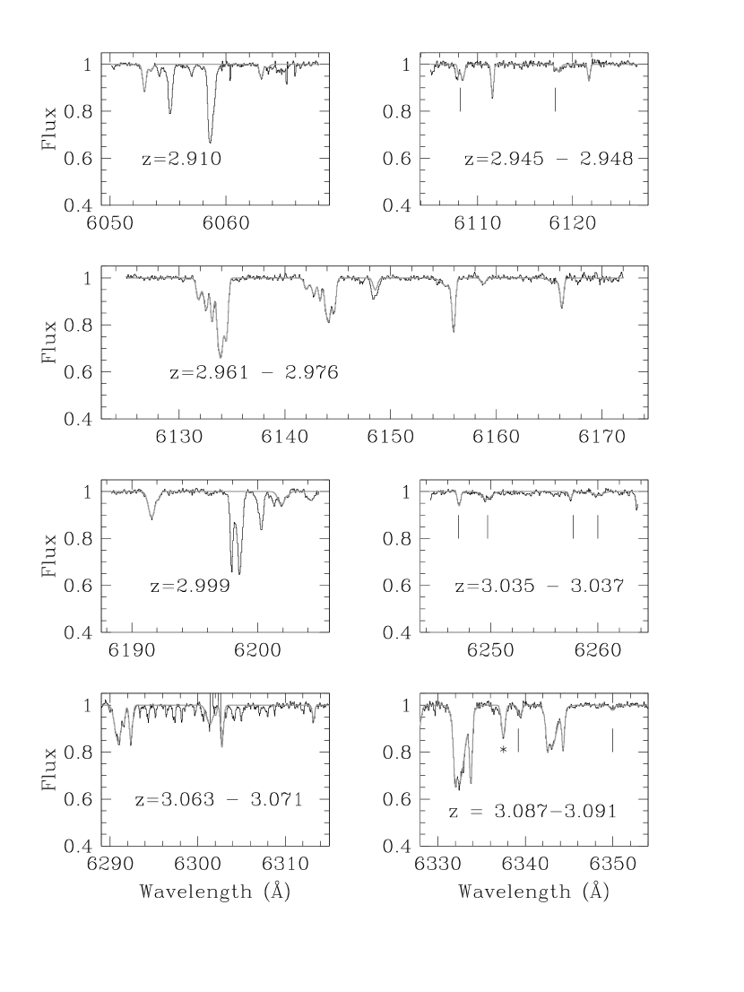
Figure 1.— Atlas of C IV doublets associated with Ly$\alpha$ lines in our working region. The $x$-axis is wavelength in Å and the $y$-axis is normalized counts. Gray lines show the profile fits with the parameters listed in Table 1. The weakest C IV systems are indicated with tick marks to guide the eye. The system marked with a ‘*’ in the bottom right hand panel is a C IV $\lambda$ 1550 line whose corresponding 1548 Å line is blended with a lower redshift system and is not shown here.

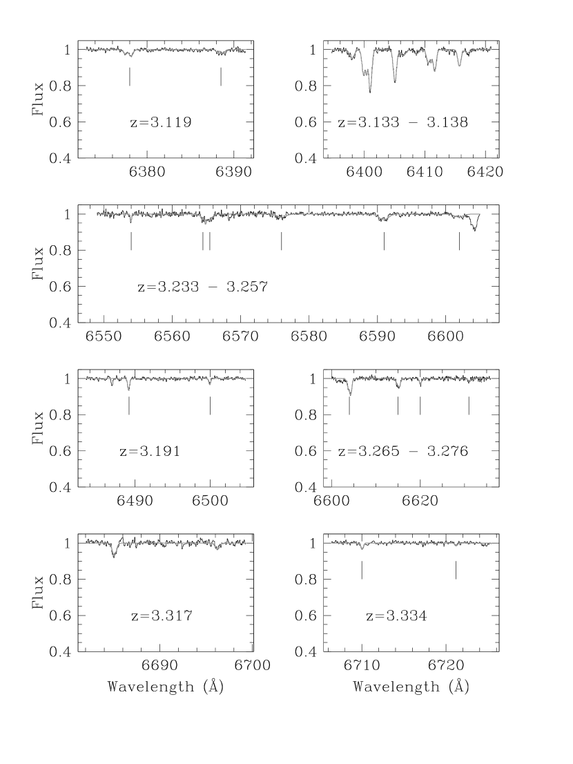
Figure 1b.— Continued

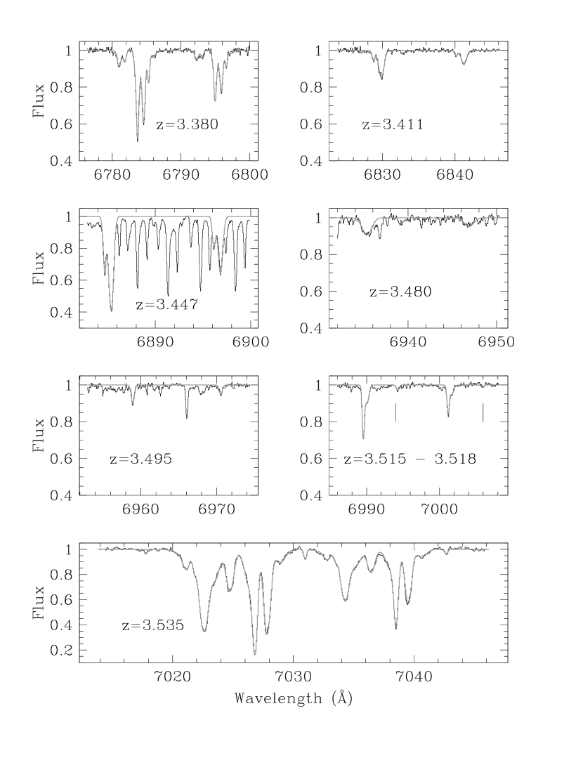
Figure 1c.— Continued

Figure 4.— Column density distribution of C IV absorbers in Q1422+231 where $f$(N) is the number of systems per column density interval per unit redshift path. The data (solid points) have been grouped into bins of width 0.3 in log $N$(C IV) for display purposes only. A maximum likelihood analysis of the distribution, assumed to be a power-law of the form $f(N)dN=BN^{-\alpha}dN$, returned a best fit index $\alpha=1.44\pm 0.05$ indicated by the solid line. At low $N$(C IV), lines with large $b$-values may not have been identified in our spectrum. We therefore simulated synthetic absorption lines for the two lowest column density bins shown here, both of which show signs of incompleteness. A total of 40 lines with $b$-values drawn at random for the observed distribution were simulated for each bin and a correction factor calculated for $N$(C IV) = 11.75 ($\times 4.4$) and $N$(C IV) = 12.05 ($\times 2.3$), based on the number of unidentifiable lines in each column density simulation. Corrected points are shown with open circles.

Figure 5.— Top: The resultant composite stack having co-added a total of 67 lines in 2 QSO sightlines, weighted by S/N. Other panels: Stacks produced from synthetic absorption spectra. The Ly$\alpha$ forests are reproduced from APM 08279+5255 and Q1422+231 and seeded with a C IV/H I ratio and offset, $\sigma_{v}$ as indicated. The $b$-values used to simulate the C IV absorption lines have been taken to be $b$(C IV) = $\frac{1}{2}$ $b$(H I). The composite spectra shown here for the model spectra represent 4 $\sigma$ detections and have equivalent widths of $\sim$ 0.15 mÅ.

Figure 6.— Top panel: Offset distribution calculated from the C IV centroids and Voigt profile fitted redshifts of H I in the metal systems in APM 08279+5255 and Q1422+231. Bottom panel: For 19 C IV systems in Q1422+231, an accurate $N$(H I) can be determined by tracing down the Lyman series. In 16 of these systems, the C IV is associated with a single H I line, the offsets for which are plotted here. For the remaining 15 C IV systems, higher order lines were either not available or were too severely blended for line fitting.

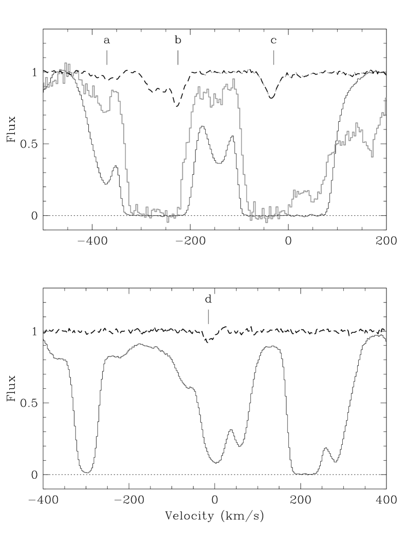
Figure 7.— Top panel: Example of absorption components in H I and C IV $\lambda 1548$ in Q1422+231. The solid black line is Ly$\alpha$ absorption and the grey line is the corresponding Ly$\beta$. The dashed line depicts the C IV absorption for 3 associated C IV complexes, marked a, b and c. The weak C IV system ‘a’ is associated with an unsaturated Ly$\alpha$ cloud and has a $\Delta z<$ 1 km s^-1  Bottom panel: A second example of an unsaturated Ly$\alpha$ line, here $\Delta z\sim$ 15 km s^-1.

Figure 8.— An illustration of how re-centering absorption lines can eliminate the effect of an offset. Top panel: Synthetic stack produced by simulating a Ly$\alpha$ forest with S/N = 200 and log C IV/H I = $-2.0$. Composite stack produced for Ly$\alpha$ lines with 13.5 $<$ log $N$(H I) $<$ 14.0. Middle panel: As above but with an added offset ($\sigma_{v}=$ 17 km/s). The unshifted stack (from the top panel) is dotted in for comparison. Bottom panel: As in the middle panel, but with the spectra re-centered on the $\tau_{max}$ pixel before stacking. Comparison with the unshifted spectrum (dotted profile) shows that almost all of the original signal is recovered.

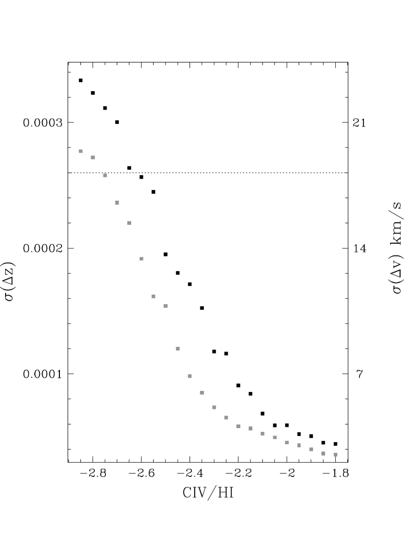
Figure 9.— Results from a pre-shift feasibility study. For each C IV/H I ratio, 1000 C IV absorption lines are produced with $b$=13 km/s and S/N = 200, corresponding to log $N$(H I) = 13.75. For each line, the offset between the true line center and the position of $\tau_{max}$ is calculated. The black squares represent the $\sigma$ of the offset distribution for each simulation of 1000 lines and is plotted in terms of both redshift and the equivalent velocity (assuming an average $z=3.45$). The gray squares are the results of the same procedure but with a 3 pixel smooth applied to the spectrum prior to locating $\tau_{max}$. The measured value of the offset determined from 55 C IV systems in APM 08279+5255 and Q1422+231 ($\sigma_{z}=2.6\times 10^{-4}$ or $\sigma_{v}=$ 17 km s^-1) is marked in the a dotted line.

Figure 10.— Results from the optical depth analyses of Q1422+231. Error bars are 1$\sigma$ as determined from the bootstrap method, as described in the text. The median absorption determined from pixel pairs separated by the C IV doublet wavelength ratio over the entire wavelength range considered (redward of Ly$\alpha$) is shown by the dotted horizontal line. The dashed diagonal line shows the optical depths expected from a spectrum with a constant log C IV/H I = $-2.6$.

Figure 11.— The optical depth distribution of Q1422+231 (solid points) is shown compared with the results from simulated spectra. Panel ‘A’: The dotted line shows the optical depth analysis of a simulated spectrum with constant log C IV/H I = $-2.6$ in all Ly$\alpha$ lines and the dot-dash line shows the results from simulated spectrum which has log C IV/H I = $-2.6$ only in log $N$(H I) $>$ 14.5 lines, with no noise added to either spectrum. Bottom panel: As for panel ‘A’ except that a S/N ratio (taken from the error array) has now been added to both spectra. All four spectra use the real Ly$\alpha$ forest of Q1422+231 and have had C IV added to the synthetic spectrum based on the fitted H I linelist. In addition all four synthetic spectra have a $\sigma_{z}$ = 2.6 $\times 10^{-4}$ and $b$(C IV) = $\frac{1}{2}b$(Ly$\alpha$). The dashed line indicates constant log C IV/H I = $-2.6$.

Figure 12.— The results from the optical depth analysis of Q1422+231 (solid points) are compared with three synthetic spectra. Top panel: open circles show the measured optical depths in a synthetic spectrum enriched solely with the detected C IV systems listed in Table 1. Middle panel: In addition to the detected C IV systems, log $N$(C IV)= 12.0 is included in all Ly$\alpha$ clouds with log $N$(H I) $>14.5$. This spectrum therefore represents the maximum amount of metals that could be ‘hidden’ below the detection limit in strong absorbers. Bottom panel: Supplementary C IV is now added in all weak (log $N$(H I)$<14.5$) Ly$\alpha$ lines with log C IV/H I = $-2.6$. Clearly, more C IV is present than currently identified directly and these optical depth results show that the data are consistent with a significant amount of C IV in low column density clouds.

Figure 13.— The optical depth results from three synthetic spectra with the Ly$\alpha$ forest re-created from the spectrum of Q1422+231. In all cases $b$(C IV) = $\frac{1}{2}b$(H I). The open squares (joined with the solid line) show the optical depths measured for an input log C IV/H I = $-2.6$ (with no scatter and no $\Delta z$) in Ly$\alpha$ lines of all H I column densities. The solid diamonds (connected with a dotted line) have C IV/H I = $-2.6$, but include a scatter of $\sigma=1\times 10^{-3}$. The spectrum represented by the solid triangles (dot-dash line) has no scatter but a redshift offset with $\sigma_{z}=2.6\times 10^{-4}$ has been included in the position of the C IV lines. Bootstrap 1$\sigma$ errors from 250 iterations are shown and points have been offset here to facilitate distinction. Clearly the effect of scatter and redshift offset on the results of this analysis are minimal.

Table 1 Details of Absorption Components Fitted to Each C IV System.

System No.	Redshift	log $N$(C IV)	$b$ (km s-1)
C1	2.90969	12.44	8.8
	2.91005	11.90	11.4
C2	2.94522	11.74	4.2
	2.94551	12.32	12.6
C3	2.94754	12.47	7.2
C4	2.96065	12.50	13.4
	2.96110	12.68	13.6
	2.96146	12.61	7.6
	2.96197	13.28	19.3
	2.96235	12.80	9.7
C5	2.97143	12.23	13.3
C6	2.97584	12.46	35.3
	2.97622	12.76	9.2
C7	2.99922	12.66	16.7
	2.99959	11.61	6.2
C8	3.03505	12.14	8.3
C9	3.03672	12.35	28.4
C10	3.06338	12.98	24.5
	3.06433	12.66	11.0
	3.06383	12.01	5.6
C11	3.07101	12.43	7.9
C12	3.08666	12.95	12.8
C13	3.08990	12.59	7.9
	3.09020	13.33	30.5
	3.09051	13.10	47.8
	3.09108	12.91	8.8
C14	3.09468	12.17	14.1
C15	3.11930	11.87	11.1
	3.11973	12.12	14.4
C16	3.13252	12.46	26.0
C17	3.13379	12.80	17.5
	3.13409	12.27	6.4
	3.13448	13.00	16.2
C18	3.13712	12.89	16.9
	3.13799	12.33	27.5
C19	3.19143	12.09	6.5
C20	3.23330	11.77	2.6
C21	3.24047	12.53	40.4
C22	3.25716	12.50	42.5
C23	3.26564	12.65	26.9
	3.26584	11.95	9.8
C24	3.27596	12.02	13.0
C25	3.31710	12.35	13.0
C26	3.33410	11.84	7.7
C27	3.37994	12.55	15.5
	3.38045	12.30	12.3
	3.38135	11.87	5.0
	3.38167	13.27	11.6
	3.38223	13.23	14.0
	3.38271	12.61	8.1
	3.38316	12.22	20.4
C28	3.41080	12.20	10.7
	3.41149	12.90	21.2
C29	3.44691	12.97	8.5
	3.44736	13.46	13.4
C30	3.47963	12.85	31.7

Table 1Continued.

System No.	Redshift	log $N$(C IV)	$b$ (km s-1)
C31	3.49488	12.46	11.4
C32	3.51465	12.83	7.5
	3.51497	12.59	15.3
C33	3.51770	11.87	10.2
C34	3.53490	12.57	34.7
	3.53505	12.69	16.0
	3.53549	12.43	7.7
	3.53599	13.69	19.9
	3.53659	13.12	21.7
	3.53738	13.22	17.2
	3.53872	13.58	9.2
	3.53937	13.58	14.1
	3.54005	12.82	25.6
	3.53848	13.33	25.0
	3.54140	12.10	4.4

Table 3Column densities for C IV enriched systems H I clouds whose Voigt profile fits could be accurately determined from Ly$\alpha$ (if unsaturated), or Ly$\beta$ and Ly$\gamma$. The C IV column densities are determined to better than 5%.

Redshift	log $N$(H I)	log $N$(C IV)	log C IV/H I
2.947	15.18$\pm$0.06	12.47	-2.71
2.999	15.77$\pm$0.05	12.70	-3.07
3.035	14.64$\pm$0.07	12.14	-2.50
3.037	14.63$\pm$0.03	12.34	-2.29
3.063	15.36$\pm$0.03	13.18	-2.18
3.071	13.85$\pm$0.01	12.43	-1.42
3.132	13.74$\pm$0.10	12.46	-1.28
3.134	15.71$\pm$0.03	13.26	-2.45
3.137	15.93$\pm$0.09	13.00	-2.93
3.191	14.89$\pm$0.20	12.09	-2.80
3.276	14.07$\pm$0.01	12.02	-2.05
3.318	13.97$\pm$0.10	12.35	-1.62
3.334	14.78$\pm$0.06	11.84	-2.94
3.382	16.70$\pm$0.40	13.68	-3.02
3.411	15.19$\pm$0.02	12.98	-2.21
3.479	15.29$\pm$0.02	12.85	-2.44
3.515	15.34$\pm$0.20	13.02	-2.32
3.518	13.29$\pm$0.03	11.87	-1.42
3.539	16.17$\pm$0.20	14.29	-1.88

References

- Bi & Davidsen (1997) Bi, H. & Davidsen, A. F. 1997, ApJ, 479, 523
- Bechtold et al. (1994) Bechtold, J., Crotts, A. P. S., Duncan, R. C., Fang, Y., 1994 ApJ, 437, 83
- Cen et al. (1994) Cen, R., Miralda-Escudé, J., Ostriker, J. P., & Rauch, M. 1994, ApJ, 437, L9
- Cowie & Songaila (1998) Cowie, L. L., & Songaila, A. 1998, Nature, 394, 44
- Cowie et al. (1995) Cowie, L. L., Songaila, A., Kim, T.-S., & Hu, E. 1995, AJ, 109, 1522
- Davé et al. (1998) Davé, R., Hellsten, U., Hernquist, L., Katz, N., Weinberg, D. H., 1998, ApJ, 509, 661
- Davé et al. (1997) Davé, R., Hernquist, L., Weinberg, D. H., Katz, N., 1997, ApJ, 477, 21
- Dinshaw et al. (1997) Dinshaw, N., Weymann, R. J., Impey, C. D., Foltz, C. B., Morris, S. L., Ake, T., 1997, ApJ, 491, 45
- Efstathiou, Schaye & Theuns (2000) Efstathiou, G., Schaye, J., & Theuns, T. 2000, Philos. Trans. R. Soc. Lond. A, in press (astro-ph/0003400)
- Ellison et al. (1999a) Ellison, S. L., Lewis, G. F., Pettini, M., Chaffee, F. H., Irwin, M. J., 1999, ApJ, 520, 456 (Paper I)
- Ellison et al. (1999b) Ellison, S. L., Lewis, G. F., Pettini, M., Sargent, W. L. W., Chaffee, F. H., Foltz, C. B., Rauch, M., Irwin, M. J., 1999, PASP, 111, 946
- Ferrara Pettini & Shchekinov (2000) Ferrara, A., Pettini, M., & Shchekinov, Y., 2000, MNRAS, in press (astro-ph/0004349)
- Gnedin (1998) Gnedin, N. Y. 1998, MNRAS, 294, 407
- Gnedin & Ostriker (1997) Gnedin, N. Y., & Ostriker, J. P. 1997, ApJ, 486, 581
- Haehnelt (1998) Haehnelt, M. G., 1998, The Young Universe: Galaxy Formation and Evolution at Intermediate and High Redshift. Edited by S. D’Odorico, A. Fontana, and E. Giallongo. ASP Conference Series; Vol. 146, p.249
- Hellsten et al. (1997) Hellsten, U., Davé, R., Hernquist, L., Weinberg D. H., & Katz, N. 1997, ApJ, 487, 482
- Hernquist et al. (1996) Hernquist, L., Katz, N., Weinberg, D. H., & Miralda-Escudé, J. 1996, ApJ, 457, L51
- Kundic et al. (1997) Kundic, T., Hogg, D. W., Blandford, R. D., Cohen, J. G., Lubin, L. M., Larkin, J. E., 1997, AJ, 114, 2276
- Lu (1991) Lu, L. 1991, ApJ, 379, 99
- Lu et al. (1998) Lu, L., Sargent, W. L. W., Barlow, T. A., & Rauch, M. 1998, submitted to ApJ, (astro-ph/9802189)
- Lu, Wolfe & Turnshek (1991) Lu, L., Wolfe, A., Turnshek, D., 1991, ApJ, 367, L19
- Lynds (1971) Lynds, R. 1971, ApJ, 164, L73
- Lynds & Stockton (1966) Lynds, C. R., & Stockton, A. N., 1966, ApJ, 144, 446
- MacLow & Ferrara (1999) MacLow, M.-M., & Ferrara A., 1999, ApJ, 513 142
- Melott (1980) Melott, A., 1980 ApJ, 268, 630
- Nath & Trentham (1997) Nath, B., & Trentham, N., 1997, MNRAS, 291, 505
- Norris, Peterson & Hartwick (1983) Norris, J., Peterson, B. A., & Hartwick, F. D. A. 1983, ApJ, 273, 450
- Ostriker & Gnedin (1996) Ostriker, J. P., & Gnedin N. Y. 1996, ApJ, 472, L63
- Ostriker & Ikeuchi (1983) Ostriker, J. P., Ikeuchi, S., 1983, ApJ, 268, 63
- Patnaik et al. (1992) Patnaik, A. R., Browne, I. W. A., Walsh, D., Chaffee, F., Foltz, C., 1992, MNRAS, 259, 1
- Petitjean & Bergeron (1994) Petitjean, P., & Bergeron, J., 1994, A&A, 283, 759
- Petry et al. (1998) Petry, C. E., Impey, C. D., Foltz, C. B., 1998, ApJ, 494, 60
- Rauch (1998) Rauch, M., 1998, ARA&A, 36, 267
- Rauch, Haehnelt & Steinmetz (1997) Rauch, M., Haehnelt, M. G., Steinmetz, M., 1997, ApJ, 481, 601
- Rauch et al. (1998) Rauch, M., Sargent, W. L. W., Barlow, T. A., 1998, ASP, 146, 167
- Rauch et al. (1999) Rauch, M., Sargent, W. L. W., Barlow, T. A., 1999, ApJ, 515, 500
- Rees (1986) Rees, M. J., 1986, MNRAS, 218, 25
- Sargent et al. (1980) Sargent W. L. W., Young, P.J., Boksenberg, A., & Tytler, D. 1980, ApJS, 42, 41
- Songaila (1997) Songaila, A. 1997, ApJL, 490, L1
- Songaila (1998) Songaila, A. 1998, AJ, 115, 2184
- Songaila & Cowie (1996) Songaila, A., & Cowie, L. L. 1996, AJ, 112, 335
- Tonry (1998) Tonry, J. L., 1998, AJ, 115, 1
- Tytler et al. (1995) Tytler, D., Fan, X.-M., Burles, S., Cottrell, L., Davis, C., Kirkman, D., & Zuo, L. 1995, QSO Absorption Lines, ed. G. Meylan (Garching, ESO), 289
- Vogt et al. (1994) Vogt, S. S. 1992, in ESO Conf. and Workshop Proc 40, High Resolution Spectroscopy with the VLT, ed. M.-H. Ulrich (Garching: ESO), 223
- Webb (1987) Webb J. K. 1987, PhD thesis, University of Cambridge