Exhaustive Study of Cosmic Microwave Background Anisotropies in Quintessential Scenarios

Abstract

Recent high precision measurements of the CMB anisotropies performed by the BOOMERanG and MAXIMA-1 experiments provide an unmatched set of data allowing to probe different cosmological models. Among these scenarios, motivated by the recent measurements of the luminosity distance versus redshift relation for type Ia supernovae, is the quintessence hypothesis. It consists in assuming that the acceleration of the Universe is due to a scalar field whose final evolution is insensitive to the initial conditions. Within this framework we investigate the cosmological perturbations for two well-motivated potentials: the Ratra-Peebles and the SUGRA tracking potentials. We show that the solutions of the perturbed equations possess an attractor and that, as a consequence, the insensitivity to the initial conditions is preserved at the perturbed level. Then, we study the predictions of these two models for structure formation and CMB anisotropies and investigate the general features of the multipole moments in the presence of quintessence. We also compare the CMB multipoles calculated with the help of a full Boltzmann code with the BOOMERanG and MAXIMA-1 data. We pay special attention to the location of the second peak and demonstrate that it significantly differs from the location obtained in the cosmological constant case. Finally, we argue that the SUGRA potential is compatible with all the recent data with a standard values of the cosmological parameters. In particular, it fits the MAXIMA-1 data better than a cosmological constant or the Ratra-Peebles potential.

]

I Introduction

Recent measurements of the luminosity distance versus redshift relation for type Ia supernovae [1], if confirmed, are compatible with an expanding (accelerating) universe driven by a new type of matter whose equation of state $p=\omega\rho$ is characterized by a negative $\omega$. One of the possible explanations is the existence of a non-zero vacuum energy, i.e. a “cosmological constant”. Another pragmatic possibility which has been proposed is to assume the existence of a yet unknown mechanism guarenteeing that the true cosmological constant vanishes, the remaining energy density being then due to the presence of a scalar field, the quintessence field, almost decoupled from ordinary matter [2, 3, 4, 5]. The main difference between a quintessence fluid and a cosmological constant comes from their equation of state where $\omega_{\Lambda}=-1$ for a cosmological constant and $-1\leq\omega_{\mathrm{Q}}\leq 0$ for the quintessence fluid.

One of the puzzles in the interpretation of these data is the extremely small value of the energy density due to the new form of matter. From the point of view of particle physics a vanishing value for the cosmological constant is one of the major challenges [6]. At present there is no known mechanism which prevents the vacuum energy from picking large values due to radiative corrections and one expects typically a contribution equal to $(\hbar c/2)\int{\mathrm{d}}{\bf k}k/(2\pi)^{3}\simeq\hbar ck_{\mathrm{m}ax}^{4}/(16\pi^{2})$, where $k_{\mathrm{m}ax}$ is a cut-off which can naturally be taken as the Planck wavenumber. This gives a contribution which is $120$ orders of magnitude above the observed one. One possibility which is often advocated is the presence of some global supersymmetry (SUSY) which would guarantee that the energy of the vacuum is zero. Unfortunately SUSY has to be broken to take into account the absence of experimental evidence in favour of particle superpartners leading to a natural contribution to the vacuum energy of order $M_{\mathrm{S}USY}^{4}$ where $M_{\mathrm{S}USY}$ is the SUSY breaking scale estimated around $1\,{\rm{TeV}}$ [7]. The measurement of a vacuum energy some $60$ orders of magnitude below this expected value indicates that some new physics must be at play here.

In the quintessence hypothesis, the small vacuum energy density is due to the rolling down of the quintessence field $Q$ along a decreasing potential. A typical potential is the Ratra-Peebles potential $V(Q)=\Lambda^{4+\alpha}/Q^{\alpha}$ [2]. From the particle physics point of view one would like to justify the existence of the quintessence field. Several natural candidates have been ruled out such as the axion-dilaton field [8], the moduli fields of toroidal compactifications in string theory [9] and finally the meson fields of supersymmetric gauge theories [10]. Nevertheless, it seems reasonnable to expect that SUSY will play a role in the solution. Within this framework it is a matter of fact that the quintessence field must be part of supergravity (SUGRA) models [10, 11]. This comes from the large value $Q\simeq m_{\mathrm{P}l}$ of the field at small redshift which implies that SUGRA corrections cannot be neglected. In [11] an effective theory approach has been used to deduce the general form of quintessence SUGRA potentials, they are of the type

$$V(Q)=\frac{\Lambda^{4+\alpha}}{Q^{\alpha}}e^{\kappa Q^{2}/2},$$ (1)

where $\kappa\equiv 8\pi G$, $G$ being the Newton constant, and where the exponential factor comprises the SUGRA corrections. $\Lambda$ and $\alpha$ are free parameters. The fine-tuning is not too severe as for typical values $\alpha=6$ the scale $\Lambda\simeq 10^{6}\,{\rm{GeV}}$ is compatible with high energy scales. Notice that the SUGRA corrections become relevant towards the end of the evolution and decouple at small $Q\ll m_{\mathrm{P}l}$. Different types of potentials can be distinguished because they lead to different values of the equation of state parameter. For example, for $\alpha=11$, the Ratra-Peebles potential is such that $\omega_{\mathrm{Q}}\simeq-0.29$ whereas the SUGRA potential gives $\omega_{\mathrm{Q}}\simeq-0.82$ [11] (for $\Omega_{\mathrm{Q}}=0.7$).

It is also worth noticing that there exists quintessence models where the field is non-minimally coupled with the metric. Such models induce time-variation of the Newton constant and are therefore already constrained, for example by observations in the solar system or by pulsar timing measurements [12, 13]. They lead to the same tracking behaviour, as stressed in Refs. [14, 15], as soon as the coupling term is proportional to a power of the potential. However, some important differences occur when the field starts dominating; for example its effective equation of state can reach extreme values such that $\omega\simeq-3$ [16]. Also, these models can lead (especially in the context of quintessential inflation [17]) to clear observable features in the gravitational waves spectrum [18].

In view of the numerous phenomenological successes of quintessence, it is relevant to deduce its consequences for Cosmic Microwave Background (CMB) anisotropies and structure formation. The aim is two–fold. First, we have to study whether quintessence leads to acceptable scenarios and, second, we have to learn how we could use high-precision measurements recently obtained by the BOOMERanG [19, 20, 21] and MAXIMA-1 [22, 23] experiments or to be performed in the near future by NASA’s Microwave Anisotropy Probe (MAP) satellite [24], ESA’s Planck satellite [25] or the Sloan Digital Sky Survey (SDSS) [26] to put constraints on the quantities characterizing quintessence like $\Omega_{\mathrm{Q}}$ or $\omega_{\mathrm{Q}}$. The second possibility has of course already been investigated for the cosmological constant case. For example, the fraction $\Omega_{\Lambda}$ of the critical density is not determined entirely from the supernovae data. Indeed, the data from the supernovae observations are degenerate in the plane $(\Omega_{\mathrm{m}},\Omega_{\Lambda})$, where $\Omega_{\mathrm{m}}$ is the matter (i.e. cold dark matter plus baryons) component preventing a clear cut determination of the fraction $\Omega_{\Lambda}$. The situation changes drastically if one includes the measurements of the CMB anisotropies [27] (even without the BOOMERanG or MAXIMA-1 data). In that case, the degeneracy is removed leading to a probable $70\%$ of the total energy density of the universe carried by the negative pressure fluid while the remaining $30\%$ are the matter components ensuring that $\Omega_{0}=1$ in agreement with a spatially flat universe. This conclusion can be drawn from the measurements of the location of the first Doppler peak. This result has been confirmed by other measurements [28, 29, 30]. Another use of combined data has been to put constraints on the equation of state parameter. However, this has been done only for constant or for very simple time-dependent $\omega_{\mathrm{Q}}$ [31, 32, 33].

CMB anisotropies and the power spectrum are calculated with the help of the theory of cosmological perturbations. Cosmological perturbations in the presence of quintessence have been studied by Ratra and Peebles but only in the tracking regime [2]. CMB multipoles moments and/or the power spectrum have already been calculated for the Ratra-Peebles potential in Ref. [34] and for other models of quintessence in Refs. [35, 36, 37, 38, 39]. One important issue is to understand whether the final evolution of the various perturbed quantities depend on the initial conditions imposed at reheating (of the inflationary type or not). Another way to put the same problem is the following: do the multipole moments depend on the value of $\delta Q(\eta_{\rm i})$ and $\delta Q^{\prime}(\eta_{\rm i})$ at initial time? In Ref. [34], it was noticed that the answer to this question is no but no explanations were provided. Here, we confirm the remark of Ref. [34] and show that this is due to the fact that the perturbed Einstein equations also possess an attractor which renders the multipole moments insensitive to the initial conditions.

One of the main purpose of this article is the study of the general properties of the multipoles moments of the CMB anisotropies in presence of the quintessence field. We present the CMB multipole moments for the Ratra-Peebles potential and, for the first time, for the SUGRA tracking potential. In addition, we also display the matter power spectrum for these two models. Recently, it has been shown by Kamionkowski and Buchalter [40] that the location of the second peak in the CMB power spectrum is an efficient way of revealing some features of the dark energy sector. Therefore, we pay special attention to this question. In particular, in Ref. [40], only the cosmological constant case was studied and it was argued that the quintessence case (the authors refer to the Ratra-Peebles potential) must not differ significantly from the cosmological constant case. In the present article, we demonstrate that this is not the case and that, as a matter of fact, quintessence leads to a different location (denoted, in the following, $l_{2}$) of the second peak. In addition, we show that the location of the second peak in the quintessence case and in the cosmological constant case can be easily distinguished. Following Ref. [40], we display the contour plots of $l_{2}$ in the plane $(\Omega_{\mathrm{m}},h)$ for the Ratra-Peebles and SUGRA tracking potentials.

The article is organized as follows. In section II, we give a description of the background evolution in terms of two physical quantities: the equation of state parameter $\omega_{\mathrm{Q}}$ and the sound velocity ${c^{2}_{\mathrm{s}}}_{\mathrm{Q}}$. In section III, we study the cosmological perturbations for the quintessence field. In section IV, we present the results of full numerical calculations with the help of a Boltzmann code developped by one of us (A.R.) for the CMB anisotropies and power spectra in the case of the Ratra-Peebles and SUGRA potentials. Then, detailed comparisons with the recent BOOMERanG [20, 21] and MAXIMA-1 [22, 23] data are performed. We end with our main conclusions in section V.

II The background evolution

We suppose that the Universe can be described by a Friedman-Lemaître-Robertson-Walker metric the spacelike sections of which are flat

$${\mathrm{d}}s^{2}=a^{2}(\eta)(-{\mathrm{d}}\eta^{2}+\delta_{ij}{\mathrm{d}}x^{i}{\mathrm{d}}x^{j}).$$ (2)

In this equation, $\eta$ is the conformal time related to the cosmic time by $a(\eta){\mathrm{d}}\eta\equiv{\mathrm{d}}t$. The matter content is as follows. The Universe is filled with a mixture of five fluids: photons ($\gamma$), neutrinos ($\nu$), baryons (${\mathrm{b}}$), cold dark matter (${\mathrm{c}dm}$) and a scalar field $Q$ named quintessence. The stress energy tensor of each of these species is the one of a perfect fluid, $T_{\mu\nu}=(p+\rho)u_{\mu}u_{\nu}+pg_{\mu\nu}$, where $u_{\mu}$ is the 4-velocity of the fluid. The energy density and the pressure of the scalar field are given by $\rho_{\mathrm{Q}}=\frac{1}{2}(Q^{\prime}/a)^{2}+V(Q)$ and $p_{\mathrm{Q}}=\frac{1}{2}(Q^{\prime}/a)^{2}-V(Q)$, where $V(Q)$ is the potential of quintessence whose shape will be very important in what follows. Each fluid is also characterized by its equation of state $p_{\rm i}\equiv\omega_{\rm i}\rho_{\rm i}$ where ${\rm i}=\gamma,\nu,{\mathrm{b}},{\mathrm{c}dm}$ or ${\mathrm{Q}}$. We have $\omega_{\gamma}=\omega_{\nu}=1/3$ and $\omega_{\mathrm{b}}=\omega_{\mathrm{c}dm}=0$. The case of $\omega_{\mathrm{Q}}$ is more complicated since this is a time-dependent function such that $-1\leq\omega_{\mathrm{Q}}\leq+1$. Its expression reads $\omega_{\mathrm{Q}}=1-2V(Q)/\rho_{\mathrm{Q}}$. The fact that $\omega_{\mathrm{Q}}$ is a time-dependent function directly comes from the fact that, for a scalar field, the sound velocity defined as [41]

$${c^{2}_{\mathrm{s}}}_{\mathrm{Q}}\equiv\frac{p_{\mathrm{Q}}^{\prime}}{\rho_{\mathrm{Q}}^{\prime}}=1+\frac{4a^{2}}{3{\mathcal{H}}Q^{\prime}}\frac{{\mathrm{d}}V(Q)}{{\mathrm{d}}Q}=-\frac{1}{3}\left(2\frac{Q^{\prime\prime}}{{\mathcal{H}}Q^{\prime}}+1\right),$$ (3)

is not equal to the equation of state parameter $\omega_{\mathrm{Q}}$. As a consequence $\omega_{\mathrm{Q}}$ has to change in time as revealed by the following equation

$$\omega_{\mathrm{Q}}^{\prime}=-3{\mathcal{H}}(1+\omega_{\mathrm{Q}})({c^{2}_{\mathrm{s}}}_{\mathrm{Q}}-\omega_{\mathrm{Q}}),$$ (4)

unless $\omega_{\mathrm{Q}}=-1$.

The evolution of the Universe can be calculated with the help of the Friedman and conservation equations

$$\frac{1}{a^{2}}{\mathcal{H}}^{2} = \frac{8\pi}{m_{\mathrm{P}l}^{2}}\sum_{i}\rho_{\rm i},$$ (5)

$$\rho_{\rm i}^{\prime} = -3{\mathcal{H}}(1+\omega_{\rm i})\rho_{\rm i},\quad{\rm i}=\gamma,\nu,{\mathrm{b}},{\mathrm{c}dm}\mbox{ or }{\mathrm{Q}},$$ (6)

where $m_{\mathrm{P}l}$ is the Planck mass and ${\mathcal{H}}\equiv a^{\prime}/a$ is related to the Hubble constant by the equation $H={\mathcal{H}}/a$. The equations of conservation simply express the fact that the energy is conserved for each species which do not interact. The equation of conservation of the quintessence field can also be written as the Klein-Gordon equation

$$Q^{\prime\prime}+2{\mathcal{H}}Q^{\prime}+a^{2}\frac{{\mathrm{d}}V}{{\mathrm{d}}Q}=0.$$ (7)

We now need to give the last piece of information necessary to have a complete description of the system, i.e. the shape of the potential $V(Q)$. In order to be an interesting theory and to represent an improvement over the current situation, quintessence has to address the following four problems: the fine-tuning problem, the coincidence problem, the equation of state problem and the model building problem. The fine-tuning problem amounts to understanding whether one can have $\Omega_{\mathrm{Q}}\simeq 0.7$ with the free parameters of the potential taking “natural” values, i.e. close to the energy scale of the theory under consideration. The coincidence problem is the question of the initial conditions: does the final value of $\rho_{\mathrm{Q}}$ strongly depend on the chosen initial values of $Q$ and $Q^{\prime}$? The equation of state problem is the question of the value of $\omega_{\mathrm{Q}}$. In order to be compatible with observational data, it should be such that $-1<\omega_{\mathrm{Q}}<0$. According to recent papers, even more stringent restrictions can be put, namely $-1<\omega_{\mathrm{Q}}<-0.6$ [29] or even $-1<\omega_{\mathrm{Q}}<-0.8$ [33]. In particular, this already rules out a network of cosmic strings since the corresponding fluid has an equation of state parameter equal to $-1/3$. Finally, the model building problem consists in justifying the shape of the potential from the high energy physics point of view. Many different shapes of potential which allow, at least partially, to solve these problems have been investigated in the litterature and Table I summarizes these proposals.

Potential	References
$\Lambda^{4+\alpha}/Q^{\alpha}$	[2]
$\Lambda^{4}e^{-\lambda Q}$	[2, 3]
$(\Lambda^{4+\alpha}/Q^{\alpha})e^{\frac{\kappa}{2}Q^{2}}$	[10, 11]
$\Lambda^{4}(\cosh\lambda Q-1)^{p}$	[43]
$\Lambda^{4}(e^{\alpha\kappa Q}+e^{\beta\kappa Q})$	[44]
$\Lambda^{4}e^{-\lambda Q}(1+A\sin\nu Q)$	[39]
$\Lambda^{4}[(Q-B)^{\alpha}+A]e^{-\lambda Q}$	[45]
$\Lambda^{4}[1+\cos(Q/f)]$	[46]

TABLE I.: Quintessence potentials that have been used in the litterature.

In particular, the first possibility has been studied thoroughly in the past years. In this article, we will mainly concentrate on the Ratra-Peebles potential [2] and the SUGRA tracking potential [10, 11].

Let us briefly see how the four questions evoked previously can be addressed with these potentials.

A The fine-tuning problem

Let us start with the fine-tuning problem which is clearly a delicate question. This problem is crucial [6] for the cosmological constant. Indeed, from very simple high energy physics considerations, one typically expects $\rho_{\Lambda}\simeq m_{\mathrm{P}l}^{4}\simeq 10^{76}\,{\rm{GeV}}^{4}$ whereas one measures $\rho_{\Lambda}\simeq\Omega_{\Lambda}\rho_{\mathrm{c}}\simeq 10^{-47}\,{\rm{GeV}}^{4}$ since the critical energy density is $\rho_{\mathrm{c}}\simeq 8.1h^{2}\times 10^{-47}\,{\rm{GeV}}^{4}$. Do we gain something in the case of quintessence? This question is controversial. For example in Ref. [42], the authors clearly answer no and write “Two proposals to explain these observations are a non-vanishing cosmological constant or a very slowly rolling scalar field, often dubbed quintessence. Both proposals, however, are plagued with formidable fine tuning problems.” However, one should look more carefully at this point. To illustrate this issue, let us consider the general argument given against quintessence. If we consider the potential $V(Q)=(m^{2}/2)Q^{2}$ then the mass of such a field, which is also the only free parameter of the potential, should be $m=\sqrt{2\Omega_{\mathrm{Q}}\rho_{\mathrm{c}}}/m_{\mathrm{P}l}\simeq 10^{-33}\,{\rm{eV}}$, a very tiny mass indeed. Justifying such a value for the free parameter $m$ is probably the same problem as justifying a very low value for $\rho_{\Lambda}$. However, such a model has never been advocated for the quintessence field. As already mentioned above, one typically considers models such that $V(Q)=\Lambda^{4+\alpha}/Q^{\alpha}$. This changes the argument. Now, the free parameter of the theory is $\Lambda$. In order to have $\rho_{\mathrm{Q}}=\Omega_{\mathrm{Q}}\rho_{\mathrm{c}}$ today, one has $\Lambda\simeq 10^{11}\,{\rm{GeV}}$, for $\alpha=11$. This time, the free parameter of the theory has a value comparable to the natural scales of high energy physics. Therefore, something has been gained and it seems unfair not to emphasize this point. On the other hand the mass of the field is given by $m=\alpha(\alpha+1)\Omega_{\mathrm{Q}}\rho_{\mathrm{c}}/m_{\mathrm{P}l}^{2}\simeq 10^{-33}\,{\rm{eV}}$ but this number should be interpreted completely differently. Here the mass $m$ is just a “by-product” and its value is naturally very small without any artificial fine-tuning of $\Lambda$. Of course the very small value of the mass implies that the quintessence field is almost completely decoupled from the other matter fields. This renders the model building issue even more acute.

B The coincidence problem

The coincidence problem as formulated in the introduction, i.e. the dependence upon the initial conditions, is solved because the Klein-Gordon equation possesses an attractor. In order to prove this property, we have to rely either on numerical calculations or on approximate methods. All the plots and numerical estimates displayed in this article will be made with the help of numerical calculations. However, it is always useful to understand the tracking property by means of analytical methods and we now turn to this question. It is convenient, for analytical calculations, to consider that there is in fact only one “background” fluid with a time dependent equation of state such that $\omega_{\mathrm{B}}=1/3$ during the radiation dominated epoch and $\omega_{\mathrm{B}}=0$ during the matter dominated era. In addition to the background fluid, we assume that there also exists the quintessence scalar field field. Following the treatment of Ratra and Peebles [2], it will be considered that this scalar field is a test field. This is a good approximation since this field must be sub-dominant in particular during Big Bang Nucleosynthesis (BBN) in order not to modify the behaviour of the scale factor and, as a consequence, not to spoil the success of BBN. This means that the behaviour of the scale factor is essentially determined by the background fluid and that $\sum_{i}\rho_{\rm i}\simeq\rho_{\mathrm{B}}$. This hypothesis breaks down at very small redshift when quintessence starts dominating the matter content of the Universe. Since quintessence is only a test field which does not interact with the background fluid, the scale factor and the quantity ${\mathcal{H}}$ can be written as

$$a(\eta)\propto\eta^{2/(1+3\omega_{\mathrm{B}})}\quad,\quad{\mathcal{H}}(\eta)=\frac{2}{(1+3\omega_{\mathrm{B}})\eta}.$$ (8)

For the sake of illustration, let us now consider the radiation dominated era where $\omega_{\mathrm{B}}=1/3$. Under the previous assumptions, the Klein-Gordon equation has a particular solution given by

$$Q_{\rm p}=Q_{0}\eta^{4/(\alpha+2)},$$ (9)

where $Q_{0}$ is a constant which depends on the free parameters of the potential, i.e. $\Lambda$ and $\alpha$. The tracking behaviour is revealed by the behaviour of small perturbations around $Q_{\rm p}$. Let us introduce the new time $\tau$ defined by $\eta\equiv e^{\tau}$ and define $u$ and $p$ by $Q=Q_{\rm p}u$ and $p={\mathrm{d}}u/{\mathrm{d}}\tau$. The Klein-Gordon equation, viewed as a dynamical system in the plane $(p,u)$, possesses a critical point $(0,1)$ and small perturbations around this point $\delta u,\delta p$ obey the following equation

$$\frac{{\mathrm{d}}}{{\mathrm{d}}\tau}\pmatrix{\delta p\cr\delta u}=\pmatrix{-\frac{\alpha+10}{\alpha+2}&-\frac{4(\alpha+6)}{\alpha+2}\cr 1&0}\pmatrix{\delta p\cr\delta u}.$$ (10)

Solutions to the equation $\mbox{det}(M-\lambda I)=0$, where $M$ is the matrix defined above, are given by

$$\lambda_{\pm}=-\frac{\alpha+10}{2(\alpha+2)}\pm\frac{i}{2(\alpha+2)}\sqrt{15\alpha^{2}+108\alpha+92}.$$ (11)

The real part of $\lambda_{\pm}$ is always negative and the critical point is a spiral point. Therefore, every solution will tend to $Q=Q_{\rm p}$ after an intermediate regime: $Q=Q_{\rm p}$ is an attractor and no fine-tuning of the initial conditions is required.

Before reaching the attractor, the quintessence field undergoes different regimes that we are now going to describe. These regimes are in fact characterized by two physical quantities already introduced previously: the equation of state parameter $\omega_{\mathrm{Q}}$ and the sound velocity ${c^{2}_{\mathrm{s}}}_{\mathrm{Q}}$. We study the case of an “overshoot”, in the terminology of Ref. [5], since this corresponds to initial conditions that are physically more relevant (in particular this includes the case of equipartition, i.e. $\rho_{\mathrm{Q}}\simeq 10^{-4}\rho_{\mathrm{B}}$ initially). We also assume that the background is radiation dominated $\omega_{\mathrm{B}}=1/3$.

Initially, the kinetic energy dominates the potential energy, i.e. $Q^{\prime 2}/(2a^{2})\gg V(Q)$. This means that the energy density redshifts as $\rho_{\mathrm{Q}}\propto 1/a^{6}$ and that the equation of state parameter is $\omega_{\mathrm{Q}}=1$. As a consequence, due to the constancy of $\omega_{\mathrm{Q}}$ and Eq. (4) (and also $\omega_{\mathrm{Q}}\neq-1$), we have ${c^{2}_{\mathrm{s}}}_{\mathrm{Q}}=1$ as well. The scalar field itself evolves like

$$Q=Q_{\rm f}-\frac{A}{a},$$ (12)

where $Q_{\rm f}$ and $A$ are constant. These constants are such that the term $A/a$ becomes rapidly small in comparison with the frozen value $Q_{\rm f}$ and we have the amusing situation that the field can be (almost) considered as frozen even if the kinetic energy still dominates. This is illustrated in Fig. 1.

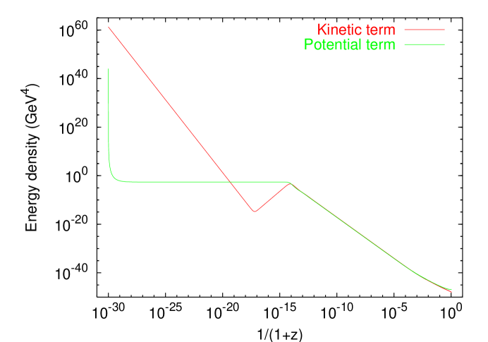
FIG. 1.: Evolution of the kinetic energy (red line) and of the potential energy $V(Q)$ (green line) from $z_{\rm i}=10^{30}$ to $z=0$.

As a consequence, during this regime the potential energy is also almost constant except at the very beginning. Using the definition of $\omega_{\mathrm{Q}}$ and ${c^{2}_{\mathrm{s}}}_{\mathrm{Q}}$, see Eq. (3), we deduce that, during the kinetic regime, we have

$$\omega_{\mathrm{Q}}-1\propto a^{6},\quad{c^{2}_{\mathrm{s}}}_{\mathrm{Q}}-1\propto a^{5}.$$ (13)

The fact that, in the parametrization adopted here, the scale factor is very small during the kinetic regime explains that there is no contradiction between these equations and the values of $\omega_{\mathrm{Q}}$ and ${c^{2}_{\mathrm{s}}}_{\mathrm{Q}}$ deduced above.

Since the kinetic energy decreases while the potential energy is almost constant, the kinetic regime cannot last forever. When the potential energy becomes larger than the kinetic one, the equation of state parameter suddenly jumps from $+1$ to $-1$ while the sound velocity still remains equal to $+1$ since Eq. (4) does not imply a change of this quantity in the case $\omega_{\mathrm{Q}}=-1$. The fact that the equation of state parameter changes before the sound velocity is explained by Eq. (13). We call this regime the transition regime. During this regime, the kinetic energy still redshifts as $1/a^{6}$ and $V(Q)$ is approximately constant but of course now $\rho_{\mathrm{Q}}\simeq V(Q)$.

Due to the second of Eq. (13), the sound velocity has also to change at some later time. This implies that the quintessence field can no longer behave according to Eq. (12). This is the starting point of the potential regime. In order to study the behaviour of the system in this regime, we need to find an expression for the second derivative of the potential. Differentiating once the definition of the sound velocity, Eq. (3), we arrive at

$$\frac{{\mathrm{d}}^{2}V(Q)}{{\mathrm{d}}Q^{2}} = \frac{3}{2}H^{2}\biggl{\{}\frac{1}{{\mathcal{H}}}{c^{2}_{\mathrm{s}}}_{\mathrm{Q}}^{\prime}$$ (14)

$$+ ({c^{2}_{\mathrm{s}}}_{\mathrm{Q}}-1)\biggl{[}\frac{{\mathcal{H}}^{\prime}}{{\mathcal{H}}^{2}}-\frac{1}{2}(3{c^{2}_{\mathrm{s}}}_{\mathrm{Q}}+5)\biggr{]}\biggr{\}}.$$ (15)

No approximation has been made in the derivation of this relation. This formula generalizes Eq. (3) of Ref. [4]. This formula will turn out to be very useful when we study the perturbations in the next section. With the scale factor given by Eqns. (8), this relation can be re-written as

$$\frac{2}{3H^{2}}\frac{{\mathrm{d}}^{2}V(Q)}{{\mathrm{d}}Q^{2}}=\frac{1}{{\mathcal{H}}}{c^{2}_{\mathrm{s}}}_{\mathrm{Q}}^{\prime}-3({c^{2}_{\mathrm{s}}}_{\mathrm{Q}}-1)(\omega_{\mathrm{B}}+{c^{2}_{\mathrm{s}}}_{\mathrm{Q}}+2).$$ (16)

In the regime we are interested in, the r.h.s of the previous formula is small. The only way to satisfy this relation is to ensure that the sound velocity changes to the constant ${c^{2}_{\mathrm{s}}}_{\mathrm{Q}}=-2-\omega_{\mathrm{B}}$. This gives ${c^{2}_{\mathrm{s}}}_{\mathrm{Q}}=-7/3$ for the radiation dominated era. This evolution is displayed in Fig. 2.

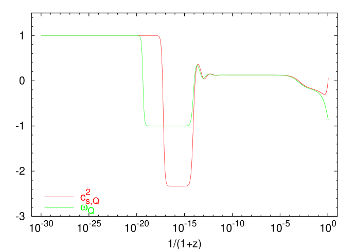
FIG. 2.: Evolution of the equation of state parameter $\omega_{\mathrm{Q}}$ (green line) and of the sound velocity ${c^{2}_{\mathrm{s}}}_{\mathrm{Q}}$ (red line) from $z_{\rm i}=10^{30}$ to $z=0$.

The fact that the sound velocity is a constant implies that the factor $(4a^{2})/(3{\mathcal{H}}Q^{\prime}){\mathrm{d}}V(Q)/{\mathrm{d}}Q$ is also a constant. Therefore, the behaviour of the quintessence field is now given by

$$Q=Q_{\rm f}+Ba^{4},$$ (17)

which implies that the kinetic energy redshifts as $a^{4}$.

Again this regime cannot last forever since the kinetic energy increases while the potential energy still remains constant. At some later time, both contributions become equal and $\omega_{\mathrm{Q}}$ and ${c^{2}_{\mathrm{s}}}_{\mathrm{Q}}$ have to change once more. This is the end of the potential regime and the beginning of the tracking regime which has already been described above. The quantities $p_{\mathrm{Q}}$, $\rho_{\mathrm{Q}}$, $V$ and the kinetic energy reach a fixed ratio such that

$$\omega_{\mathrm{Q}}={c^{2}_{\mathrm{s}}}_{\mathrm{Q}}=-\frac{2-\alpha\omega_{B}}{2+\alpha}.$$ (18)

The definitions of the different regimes and the corresponding evolutions of the physically relevant quantities are summed up in Table II.

Regime	$Q^{\prime 2}/(2a^{2})$	$V(Q)$	$Q$	$\omega_{\mathrm{Q}}$	${c^{2}_{\mathrm{s}}}_{\mathrm{Q}}$
Kinetic	$1/a^{6}$	$a^{0}$	$Q_{\rm f}-A/a$	$1$	$1$
Transition	$1/a^{6}$	$a^{0}$	$Q_{\rm f}-A/a$	$-1$	$1$
Potential	$a^{4}$	$a^{0}$	$Q_{\rm f}+Ba^{4}$	$-1$	$-7/3$
Tracking	$a^{-3(1+\omega_{\mathrm{Q}})}$	$a^{-3(1+\omega_{\mathrm{Q}})}$	$a^{4/(\alpha+2)}$	$\frac{\alpha\omega_{\mathrm{B}}-2}{\alpha+2}$	$\omega_{\mathrm{Q}}$

TABLE II.: Summary of the different regimes described in the text.

C The equation of state parameter problem

The third question evoked previously was the question of the value of the parameter $\omega_{\mathrm{Q}}$ today. As already mentioned, this is an important issue since constraints on this quantity are already available. This problem is also solved by quintessence in the sense that we always have $-1<\omega_{\mathrm{Q}}<0$. Here, however, it is relevant to distinguish between the Ratra-Peebles potential and the SUGRA potential. With the first potential, it seems difficult to reach sufficiently small value of $\omega_{\mathrm{Q}}$. On the other hand, this is automatically achieved in the second case. The reason for this is the presence of the factor $\exp(\kappa Q^{2}/2)$ in the potential, a generic feature of SUGRA-based potentials, which drives $\omega_{\mathrm{Q}}$ towards $-1$. For $\alpha=11$ and $\Omega_{\mathrm{c}dm}\simeq 0.3$, the prediction is $\omega_{\mathrm{Q}}\simeq-0.82$ a value in agreement with the current data [10, 11].

D The model building problem

From the particle physics point of view, one would like to justify the existence of the quintessence field and the shapes of the (so far) phenomenological potentials. Several attempts have already been made in the framework of supersymmetric field theory. In particular, it was shown by Binétruy [8] that the Ratra-Peebles potential can be recovered in the context of global SUSY. However, as already mentioned, SUGRA corrections must be taken into account and this implies that the corresponding potential can be of the type of the SUGRA tracking potential displayed in Eq. (1) which leads to a better agreement with the available data.

Nevertheless, it should be clear that considerable problems remain to be addressed in order to reach a satisfactory situation [47, 48]. Maybe the most crucial question is the problem of SUSY breaking. SUSY must certainly be broken but the models evoked previously do not take into account this basic fact. This could have dramatic consequences and modify the shape of the potential which is so important in order to solve the three previous problems.

III The cosmological perturbations

We now turn to the study of the cosmological perturbations. A detailed study has already been performed by Ratra and Peebles in Ref. [2] but only for the tracking regime. Cosmological perturbations in a fluid with a constant negative equation of state parameter have been investigated in Ref. [49]. In this article, we study the cosmological perturbations (in the long wavelength approximation) in all the regimes previously described and point out some additional properties. The evolution of the cosmological perturbations mainly depends on the equation of state parameter and the sound velocity. We have shown in the previous section that they can be considered as constant in each regime. This will simplify the analysis a lot.

The fate of the perturbations depends on the initial conditions. It has been noticed for the first time in Ref. [34] that “the observable fluctuation spectrum is insensitive to a broad range of initial conditions, including the case in which the amplitudes of $\delta Q$, $\delta Q^{\prime}$ are set by inflation”. In that paper, the authors choose $\delta Q=\delta Q^{\prime}=0$ initially (in the synchronous gauge). We demonstrate, in this section, that the insensitivity of the spectrum described in Ref. [34] has an origin similar to the insensitivity of the background properties with respect to the initial conditions $Q$ and $Q^{\prime}$, namely the presence of an attractor for the perturbed quantities. We prove that during all the four regimes undergone by the quintessence field, the attractor is characterized by a “spiral fixed point” as it is the case for the background.

A General framework

Without loss of generality, the perturbed line element can be written in the synchronous gauge. In this class of coordinates systems, scalar perturbations are completely described by two arbitrary functions. The spatial dependence of the perturbations is given by $X(x^{i})$ which is the eigenfunction of the Laplace operator on the flat spacelike hypersurfaces. There exists two ways to construct a two rank tensor from a scalar function : either by multiplying it by the spatial background flat metric $\delta_{ij}$ or by differentiating it twice. The two arbitrary functions mentioned above are simply the coefficients of these two terms in a Fourier expansion. Therefore, the perturbed metric can be expressed as [50]

$${\mathrm{d}}s^{2}=a^{2}(\eta)\biggl{\{} - {\mathrm{d}}\eta^{2}+\biggl{[}\biggl{(}1+h(\eta)X\biggr{)}\delta_{ij}$$ (19)

$$+ h_{l}(\eta)\frac{1}{k^{2}}X_{,i,j}\biggr{]}{\mathrm{d}}x^{i}{\mathrm{d}}x^{j}\biggr{\}}.$$ (20)

In this equation, the dimensionless quantity ${\bf k}$ is the comoving wavevector related to the physical wavevector ${\bf k}^{\rm phys}$ through the relation ${\bf k}^{\rm phys}\equiv{\bf k}/a(\eta)$. As a consequence of Einstein equations, perturbations in the metric are coupled to perturbations in the different matter components. We choose to write the perturbed stress-energy tensor according to [50]

$$T^{0}{}_{0} = -\frac{\epsilon_{1}}{a^{2}}X,\quad T^{0}{}_{i}=\frac{\xi^{\prime}}{a^{2}}X_{,i},\quad T^{i}{}_{0}=-\frac{\xi^{\prime}}{a^{2}}X^{,i},$$ (21)

$$T^{i}{}_{j} = \frac{p_{1}}{a^{2}}X\delta^{i}{}_{j},$$ (22)

where we have assumed that the longitudinal pressure $p_{l}$ vanishes for each component. As for the background, one considers that the Universe is filled with two fluids: the background fluid, an hydrodynamical perfect fluid which is either radiation or dust (again, the corresponding quantities will carry the index ${\mathrm{B}}$) and a scalar field $Q$ describing the quintessence field (in this case the corresponding quantities will carry the index ${\mathrm{Q}}$). The perturbed Einstein equations which govern the evolution of the quantities $h$ and $h_{l}$ are given by:

$$3{\mathcal{H}}h^{\prime}+k^{2}h-{\mathcal{H}}h_{l}^{\prime} = \kappa\epsilon_{1{\mathrm{B}}}+\kappa\epsilon_{1{\mathrm{Q}}},$$ (23)

$$h^{\prime} = \kappa\xi^{\prime}_{\mathrm{B}}+\kappa\xi^{\prime}_{\mathrm{Q}},$$ (24)

$$-h^{\prime\prime}-2{\mathcal{H}}h^{\prime} = \kappa p_{1{\mathrm{B}}}+\kappa p_{1{\mathrm{Q}}},$$ (25)

$$h_{l}^{\prime}+2{\mathcal{H}}h_{l}^{\prime}-k^{2}h = 0.$$ (26)

Finally, it turns out to be more convenient to work with the density contrast $\delta$ and the velocity divergence $\theta$ defined by the equations:

$$\delta\equiv\frac{\epsilon_{1}}{a^{2}\epsilon_{0}}\quad,\quad\xi^{\prime}\equiv-\frac{a^{3}\epsilon_{0}}{k^{2}}(1+\omega)\theta.$$ (27)

In the following, we study analytically the time evolution of the density contrast for the background fluid and for quintessence in the long wavelength limit.

B The background fluid

The equations satisfied by the background density contrast and divergence can be obtained either from combinations of the Einstein equations (23-26) or, more directly, from the conservation of the perturbed background fluid stress-energy tensor (since the background fluid and quintessence only interact gravitationally). They read:

$$\delta_{\mathrm{B}}^{\prime}+a(1+\omega_{\mathrm{B}})\theta_{\mathrm{B}}+\frac{1+\omega_{\mathrm{B}}}{2}(3h^{\prime}-h_{l}^{\prime}) = 0,$$ (28)

$$\theta_{\mathrm{B}}^{\prime}+(2-3\omega_{\mathrm{B}}){\mathcal{H}}\theta_{\mathrm{B}}-\frac{k^{2}{c^{2}_{\mathrm{s}}}_{B}}{(1+\omega_{\mathrm{B}})a}\delta_{\mathrm{B}} = 0.$$ (29)

These two equations are equivalent to Eqns. (7.15) and (7.16) of Ref. [2]. From them, we can derive the relation

$$3h^{\prime\prime}-h_{l}^{\prime\prime}=\frac{-2}{1+\omega_{\mathrm{B}}}\delta_{\mathrm{B}}^{\prime\prime}+2(1-3\omega_{\mathrm{B}})a^{\prime}\theta_{\mathrm{B}}-\frac{2k^{2}{c^{2}_{\mathrm{s}}}_{B}}{1+\omega_{\mathrm{B}}}\delta_{\mathrm{B}},$$ (30)

where we have assumed that $\omega_{\mathrm{B}}$ is a constant. On the other hand, from the Einstein equations we get

$$-(3h^{\prime\prime}-h_{l}^{\prime\prime})-{\mathcal{H}}(3h^{\prime}-h_{l}^{\prime})$$ (31)

$$=3{\mathcal{H}}^{2}\biggl{[}(1+3c_{\ell{\mathrm{B}}}^{2})\Omega_{\mathrm{B}}\delta_{\mathrm{B}}+(1+3c_{\ell{\mathrm{Q}}}^{2})\Omega_{\mathrm{Q}}\delta_{\mathrm{Q}}\biggr{]},$$ (32)

where $c_{\ell{\mathrm{Q}}}^{2}\equiv p_{1{\mathrm{Q}}}/\epsilon_{1{\mathrm{Q}}}$ which needs not to coincide with the definition of ${c^{2}_{\mathrm{s}}}_{\mathrm{Q}}$. In order to derive the formula satisfied by the density contrast of the background fluid in the long wavelength limit, we neglect the term proportional to $k^{2}$ in Eq. (30) and we use the fact that $\Omega_{\mathrm{Q}}\ll\Omega_{\mathrm{B}}$. Then, straightforward manipulations lead to

$$\delta_{\mathrm{B}}^{\prime\prime}+{\mathcal{H}}\delta_{\mathrm{B}}^{\prime} - \frac{3}{2}{\mathcal{H}}^{2}(1+3\omega_{\mathrm{B}})(1+\omega_{\mathrm{B}})\delta_{\mathrm{B}}$$ (33)

$$= -3{\mathcal{H}}\omega_{\mathrm{B}}(1+\omega_{\mathrm{B}})a\theta_{\mathrm{B}},$$ (34)

where we used the fact that $c_{\ell{\mathrm{B}}}^{2}=\omega_{\mathrm{B}}$ for an hydrodynamical fluid. This equation shows that the evolution of the background density contrast is essentially unaffected by the presence of quintessence. This is of course an expected result since we have assumed $\Omega_{\mathrm{Q}}\ll\Omega_{\mathrm{B}}$. The general solution to Eq. (33) can be easily found and reads

$$\delta_{\mathrm{B}}(\eta)=A_{1}\biggl{(}\frac{a}{a_{0}}\biggr{)}^{x_{+}}+A_{2}\biggl{(}\frac{a}{a_{0}}\biggr{)}^{x_{-}}$$ (35)

$$+ \frac{\omega_{\mathrm{B}}(1+\omega_{\mathrm{B}})(1+3\omega_{\mathrm{B}})a_{0}\theta_{{\mathrm{B}}0}\eta_{0}}{(1-\omega_{\mathrm{B}})(1+6\omega_{\mathrm{B}})}\biggl{(}\frac{a}{a_{0}}\biggr{)}^{(9\omega_{\mathrm{B}}-1)/2},$$ (36)

where we have defined

$$x_{\pm} \equiv -\frac{(1-3\omega_{\mathrm{B}})}{4}$$ (38)

$$\pm\frac{1}{4}\sqrt{(1-3\omega_{\mathrm{B}})^{2}+24(1+\omega_{\mathrm{B}})(1-3\omega_{\mathrm{B}})}.$$

The results for the radiation dominated and matter dominated epochs are summarized in Table III.

$\omega_{\mathrm{B}}$	$x_{-}$	$x_{+}$	$(9\omega_{\mathrm{B}}-1)/2$
$1/3$	$-2$	$2$	$1$
$0$	$-3/2$	$1$	$-1/2$

TABLE III.: Time dependence of the background fluid density contrast during radiation and matter dominated era

These results are consistent with those obtained in Ref. [51]. In particular, it can be shown that the branch $\delta_{\mathrm{B}}\propto a^{x_{-}}$ corresponds in fact to a residual gauge mode, i.e. there exists a synchronous system of coordinates such that this mode can be removed and therefore must not be considered as a physical mode.

C Quintessential perturbations

We now describe how the long wavelength quintessential perturbations evolve with time. A similar study has already been performed by Ratra and Peebles but only on the tracking solution. We give here a complete description of the evolution of the quintessence density contrast in the four regimes defined in the previous section. In addition, we prove that there exists an attractor for the perturbations as it is the case for the background solution. As a consequence, the final value of the density contrast is always the same whatever the initial conditions are.

In order to obtain the fundamental equations to be solved, we can proceed as for the background fluid. However, it is important to notice that the link between the perturbed energy density and the perturbed pression, which is just a constant for the background fluid, is more complicated in the case of quintessence. In general, we can write $p_{1{\mathrm{Q}}}={c^{2}_{\mathrm{s}}}_{\mathrm{Q}}\epsilon_{1{\mathrm{Q}}}+a^{2}\tau\delta S$ where the second term represents entropy perturbations. In the synchronous gauge, we obtain

$$p_{1{\mathrm{Q}}}={c^{2}_{\mathrm{s}}}_{\mathrm{Q}}\epsilon_{1{\mathrm{Q}}}+(1-{c^{2}_{\mathrm{s}}}_{\mathrm{Q}})\frac{1}{\kappa}(h_{l}^{\prime\prime}+{\mathcal{H}}h_{l}^{\prime}).$$ (39)

We can now establish the equations satisfied by the quintessence density contrast and divergence. The conservation of the perturbed stress-energy tensor leads to

$$\delta_{\mathrm{Q}}^{\prime}+3\alpha({c^{2}_{\mathrm{s}}}_{\mathrm{Q}}-\omega_{\mathrm{Q}})\delta_{\mathrm{Q}}+a(1+\omega_{\mathrm{Q}})\theta_{\mathrm{Q}}$$ (40)

$$+ \frac{1}{2}(1+\omega_{\mathrm{Q}})(3h^{\prime}-h_{l}^{\prime})=\frac{{\mathcal{H}}^{-1}}{\Omega_{\mathrm{Q}}}({c^{2}_{\mathrm{s}}}_{\mathrm{Q}}-1)(h_{l}^{\prime\prime}+{\mathcal{H}}h_{l}^{\prime}),$$ (42)

$$\theta_{\mathrm{Q}}^{\prime}+(2-3\omega_{\mathrm{Q}})\alpha\theta_{\mathrm{Q}}-\frac{k^{2}{c^{2}_{\mathrm{s}}}_{\mathrm{Q}}}{(1+\omega_{\mathrm{Q}})a}\delta_{\mathrm{Q}}$$

$$= -\frac{\omega_{\mathrm{Q}}^{\prime}}{1+\omega_{\mathrm{Q}}}\theta_{\mathrm{Q}}+\frac{(1-{c^{2}_{\mathrm{s}}}_{\mathrm{Q}})k^{2}}{3a{\mathcal{H}}^{2}(1+\omega_{\mathrm{Q}})\Omega_{\mathrm{Q}}}(h_{l}^{\prime\prime}+{\mathcal{H}}h_{l}^{\prime}).$$ (43)

In these two equations, no approximation have been made: they are valid for any wavenumber, any equation of state parameter and sound velocity. In practice, it turns out to be more convenient to use the perturbed Klein-Gordon equation to analyse the problem. This can be obtained directly from the first of the two previous equations if one notices that the quantities describing the perturbed scalar field stress-energy tensor can be expressed in terms of the perturbed scalar field $\delta Q(\eta,{\bf x})$ according to

$$\epsilon_{1{\mathrm{Q}}} = Q^{\prime}\delta Q^{\prime}+a^{2}\delta Q\frac{{\mathrm{d}}V(Q)}{{\mathrm{d}}Q},$$ (44)

$$\xi_{{\mathrm{Q}}}^{\prime} = -Q^{\prime}\delta Q,$$ (45)

$$p_{1{\mathrm{Q}}} = Q^{\prime}\delta Q^{\prime}-a^{2}\delta Q\frac{{\mathrm{d}}V(Q)}{{\mathrm{d}}Q}.$$ (46)

Inserting the corresponding expression for the density contrast and the divergence in Eq. (40), we get

$$\delta Q^{\prime\prime}+2{\mathcal{H}}\delta Q^{\prime}+\biggl{[}k^{2}+a^{2}\frac{{\mathrm{d}}^{2}V(Q)}{{\mathrm{d}}Q^{2}}\biggr{]}\delta Q+\frac{Q^{\prime}}{2}(3h^{\prime}-h_{l}^{\prime})=0.$$ (47)

This is similar to Eq. (7.20) of Ref. [2]. One can check that Eq. (42) is automatically verified since it is equivalent to the unperturbed Klein-Gordon equation (times an unimportant factor). Using Eq. (28) to express the factor $3h^{\prime}-h_{l}^{\prime}$ and neglecting the $k^{2}$ term, we arrive at

$$\delta Q^{\prime\prime}+2{\mathcal{H}}\delta Q^{\prime}+a^{2}\frac{{\mathrm{d}}^{2}V(Q)}{{\mathrm{d}}Q^{2}}\delta Q=Q^{\prime}a\theta_{\mathrm{B}}+\frac{Q^{\prime}}{1+\omega_{\mathrm{B}}}\delta_{\mathrm{B}}^{\prime}.$$ (48)

We are now going to analyse this equation in detail. We now need to utilize the general expression for the second derivative of the potential, Eq. (14). On the tracking solution, we have $\omega_{\mathrm{Q}}={c^{2}_{\mathrm{s}}}_{\mathrm{Q}}$ and $\omega_{\mathrm{Q}}=(-2+\alpha\omega_{\mathrm{B}})/(2+\alpha)$ and this equation reduces to

$$\frac{{\mathrm{d}}^{2}V(Q)}{{\mathrm{d}}Q^{2}}=\frac{9}{2}H^{2}\frac{\alpha+1}{\alpha}(1-\omega_{\mathrm{Q}}^{2}).$$ (49)

For our purpose, as proven in the previous section, it is sufficient to consider a regime where ${c^{2}_{\mathrm{s}}}_{\mathrm{Q}}$ is constant and where the scalar field is a test field. Under these conditions, we obtain

$$\frac{{\mathrm{d}}^{2}V(Q)}{{\mathrm{d}}Q^{2}}=\frac{3}{4}H^{2}(1-{c^{2}_{\mathrm{s}}}_{\mathrm{Q}})(6+3\omega_{\mathrm{B}}+3{c^{2}_{\mathrm{s}}}_{\mathrm{Q}}).$$ (50)

Let us now concentrate on the homogeneous part of Eq. (48). Using the previous equation, it can be expressed as

$$\delta Q^{\prime\prime}+\frac{4}{1+3\omega_{\mathrm{B}}}\frac{1}{\eta}\delta Q^{\prime}$$ (51)

$$+ \frac{3}{(1+3\omega_{\mathrm{B}})^{2}}\frac{1}{\eta^{2}}(1-{c^{2}_{\mathrm{s}}}_{\mathrm{Q}})(6+3\omega_{\mathrm{B}}+3{c^{2}_{\mathrm{s}}}_{\mathrm{Q}})\delta Q=0.$$ (52)

This linear equation can easily be solved: its solutions are just power law of the conformal time. However, in order to show explicitly the complete analogy with the background attractor, we choose to analyse it in a rather roundabout way. Let us proceed exactly as for the unperturbed Klein-Gordon equation [see the discussion around Eq. (10)]. We define the time $\tau$ by $\eta\equiv e^{\tau}$ and introduce the quantity $\delta u$ and $\delta p$ defined by $\delta u\equiv\delta Q$ and $\delta p\equiv{\mathrm{d}}(\delta Q)/{\mathrm{d}}\tau$. Then, Eq. (51) can re-expressed as

$$\frac{{\mathrm{d}}}{{\mathrm{d}}\tau}\pmatrix{\delta p\cr\delta u}$$ (53)

$$=\pmatrix{\frac{3(\omega_{\mathrm{B}}-1)}{1+3\omega_{\mathrm{B}}}&\frac{9({c^{2}_{\mathrm{s}}}_{\mathrm{Q}}-1)}{(1+3\omega_{\mathrm{B}})^{2}}(2+\omega_{\mathrm{B}}+{c^{2}_{\mathrm{s}}}_{\mathrm{Q}})\cr 1&0}\pmatrix{\delta p\cr\delta u}.$$ (54)

The form of this equation clearly shows the complete analogy with Eq. (10). The eigenvalues of the system are found by solving the equation $\mbox{det}(M-\lambda I)=0$, where $M$ is the matrix defined above and $I$ the identity matrix. Straigthforwards calculations show that the solutions are given by

$$\lambda_{\pm}=\frac{3}{2}\frac{\omega_{\mathrm{B}}-1}{1+3\omega_{\mathrm{B}}}\biggl{[}1\pm\sqrt{1+4\frac{{c^{2}_{\mathrm{s}}}_{\mathrm{Q}}-1}{(\omega_{\mathrm{B}}-1)^{2}}(2+\omega_{\mathrm{B}}+{c^{2}_{\mathrm{s}}}_{\mathrm{Q}})}\biggr{]}.$$ (55)

Of course, this is just a simple rephrasing of the fact that the solution of Eq. (51) is $\delta Q\propto A_{+}\eta^{\lambda_{+}}+A_{-}\eta^{\lambda_{-}}$. The presence of an attractor is linked to the negative sign of the real part of $\lambda_{\pm}$. It is easy to see that the real part is always negative in all four regimes, in particular this is true for any value of $\alpha$. This is displayed in Fig. 3 in the plane $(\omega_{\mathrm{B}},{c^{2}_{\mathrm{s}}}_{\mathrm{Q}})$. The green and purple regions are the regions where these real parts are negative. The green region is the region where the argument of the square root is negative, i.e. where the square root is an imaginary number. The exact “trajectories” of the system for the usual tracking potential (short line) and for the SUGRA tracking potential (long line) are also shown for the case $\alpha=11$. They have been obtained by full numerical integration. The remarkable property is that these trajectories are always in the stable region. This means that, in each region, the system tends to an attractor which is given by the inhomogeneous part of the perturbed Klein-Gordon equation. The system starts at $\omega_{\mathrm{B}}=1/3$ and goes from ${c^{2}_{\mathrm{s}}}_{\mathrm{Q}}=1$ to ${c^{2}_{\mathrm{s}}}_{\mathrm{Q}}=-7/3$. Then, the system approaches the transition to the matter dominated era and leaves the vertical line. Finally, it stops when the redshift vanishes at $\omega_{\mathrm{B}}\simeq-0.29$ for the tracking potential and at $\omega_{\mathrm{B}}\simeq-0.82$ for the SUGRA tracking potential. The two lines separate when the exponential factor becomes important in the SUGRA tracking potential.

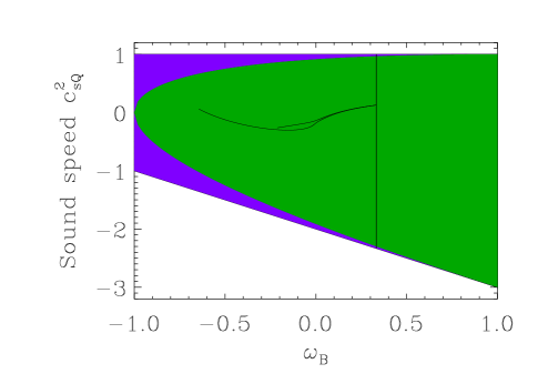
FIG. 3.: Stability region for the quintessential perturbations. The green (lightgrey) and the purple regions (darkgrey) constitute the stable region. The green region is the region where the square root is an imaginary number. Two trajectories of the system for the tracking potential (shortest line) and the SUGRA tracking potential (longest line) are also displayed for the value $\alpha=11$.

The conclusion is that the final value of the quintessence perturbations is insensitive to the initial conditions, a property completely similar to what has been shown in Ref. [5] for the background. Strictly speaking, this property has been demonstrated for long wavelength modes only. However, we have checked by numerical calculations that this is also true for shorter wavelength modes. Having proven that the final result does not depend on the initial conditions of the quintessence perturbations, we can now proceed further and embark in a rather detailed study of the CMB anisotropies predictions in the presence of quintessence.

IV Predictions for the power spectrum and the multipole moments

The presence of cosmological perturbations induces directional variations in the CMB photon redshift. This is the so-called Sachs-Wolfe effect [52]. Since these variations are the same regardless of the wavelength of the photons, they translate into variations in the temperature of the black body on the celestial sphere. Their amplitude has been measured by the COBE satellite and is of the order of magnitude $\delta T/T_{0}\simeq 10^{-5}$ [53]. The detailed angular structure of the CMB anisotropies is usually characterized by the two-point correlation function which can be expanded according to

$$\biggl{\langle}\frac{\delta T}{T}({\bf e}_{1})\frac{\delta T}{T}({\bf e}_{2})\biggr{\rangle}=\frac{1}{4\pi}\sum_{l}(2l+1)C_{l}P_{l}(\cos\gamma),$$ (56)

where $\gamma$ is the angle between the directions ${\bf e}_{1}$ and ${\bf e}_{2}$ and $P_{l}$ is a Legendre polynomial. The coefficients $C_{l}$ are the multipole moments. In what follows, we will be mainly interested in the so-called band power $\delta T_{l}$ defined by the following expression

$$\delta T_{l}\equiv T_{0}\sqrt{l(l+1)\frac{C_{l}}{2\pi}},$$ (57)

where $T_{0}\simeq 2.7\,{\rm{K}}$. The band power has now been measured on a wide range of angular scales from $10^{\prime}$ to $90^{\circ}$ corresponding roughly to $l\in[2,700]$. Almost $80$ data points have been measured. Recently new data obtained by the balloon-borne experiments BOOMERanG [20, 21] and MAXIMA-1 [22, 23] have been published. They clearly show a detection of the first Doppler peak at the expected angular scale $\simeq 1^{\circ}$ corresponding to the size of the Hubble radius at recombination.

On the theoretical side, the multipoles moments depend on the initial spectra for scalar and tensor modes and on how the perturbations evolve from the initial time (after inflation) until now. This evolution is determined by the values of the cosmological parameters, i.e. by the value of the Hubble constant ($h$), of the total amount of matter present in our Universe ($\Omega_{0}$), of the cosmological constant ($\Omega_{\Lambda}$), of the baryons density parameter ($\Omega_{\mathrm{b}}$) and of the cold dark matter density parameter ($\Omega_{\mathrm{c}dm}$). Constraints already exist on some of these parameters. In particular, as already mentioned above, $\Omega_{\Lambda}\simeq 0.7$ according to the SNIa measurements and $h^{2}\Omega_{\mathrm{b}}\simeq 0.019\pm 0.002$ according to BBN [54, 55]. We also assume $\Omega_{0}=1$ in agreement with the inflation paradigm which has been confirmed by the recent CMB anisotropy measurements. For the initial spectra, it is traditional to assume that they are of the power-law form

$$k^{3}P_{\Phi}(k)=A_{\mathrm{S}}k^{n_{\mathrm{S}}-1},\quad k^{3}P_{\rm h}(k)=A_{\mathrm{T}}k^{n_{\mathrm{T}}},$$ (58)

where the scalar and tensor spectral indices $n_{\mathrm{S}}$ and $n_{\mathrm{T}}$ are related by $n_{\mathrm{S}}-1=n_{\mathrm{T}}$. This last equation is also valid for zeroth order slow-roll inflation. It should be noticed that, a priori, this choice is not the most relevant one since slow-roll inflation is certainly more physically motivated. For spectral indices close to $n_{\mathrm{S}}=1$, we expect a small difference. This is no longer true for larger tilts. Inflation predicts the presence of gravitational perturbations and the tensor to scalar amplitude ratio is given by

$$\frac{A_{\mathrm{T}}}{A_{\mathrm{S}}}\simeq-\frac{200}{9}n_{\mathrm{T}}.$$ (59)

This equation is valid for power-law inflation with $n_{\mathrm{T}}$ not too large or for zeroth order slow-roll inflation. A last remark is in order at this point. All the plots displayed in this article are COBE normalized in the following way: the position of the Sachs-Wolfe plateau is tuned such that it best fits the COBE data points. In practice, this almost amounts to normalize the spectrum to $C_{10}$.

In this section, we first study the general properties of the multipoles moments in the quintessence cold dark matter model (QCDM) and point out the main differences with the standard cold dark matter (sCDM) and the cosmic concordance model ($\Lambda$CDM). We also display the corresponding baryonic matter power spectra, given by

$$|\delta(k)|^{2}\equiv\biggl{|}\frac{\delta\rho_{\mathrm{b}}}{\rho_{\mathrm{b}}}\biggr{|}^{2},$$ (60)

which is the square of the Fourier transform of the baryonic density contrast. Then, we compare the predictions of the QCDM model for the Ratra-Peebles and SUGRA tracking potentials with the COBE [53], BOOMERanG [20, 21], MAXIMA-1 [22, 23] and Saskatoon [56] data. We do not attempt to perform a detailed statistical analysis but we rather indicate roughly how the different models can fit the observational data.

We now turn to simple considerations about the shape of the CMB spectrum. The corresponding band power for the Ratra-Peebles and SUGRA potentials are displayed in Figs. 4 and 5 for $h=0.5$, $\Omega_{\mathrm{b}}=0.05$, $\Omega_{\mathrm{Q}}=0.7$, $\Omega_{\mathrm{c}dm}=1-\Omega_{\mathrm{b}}-\Omega_{\mathrm{Q}}$, $n_{\mathrm{S}}=0.99$ and the tensor contribution neglected. The former set of cosmological parameters has been chosen just for the sake of illustration and discussion.

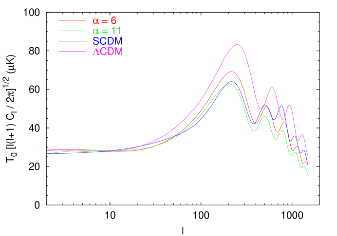
FIG. 4.: Multipole moments for the Ratra-Peebles potential for two values of $\alpha$, $\alpha=6$ (red curve) and $\alpha=11$ (green curve) and with cosmological parameters equal to $h=0.5$, $\Omega_{\mathrm{b}}=0.05$, $\Omega_{\mathrm{Q}}=0.7$, $\Omega_{\mathrm{c}dm}=1-\Omega_{\mathrm{b}}-\Omega_{\mathrm{Q}}$, $n_{\mathrm{S}}=0.99$, $A_{\mathrm{T}}=0$. The curves are compared with those obtained in the SCDM model (blue curve) and in the $\Lambda$CDM model (pink curve).

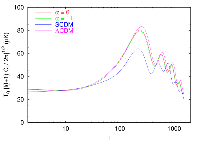
FIG. 5.: Multipole moments for the SUGRA potential for two values of $\alpha$, $\alpha=6$ (red curve) and $\alpha=11$ (green curve) and with cosmological parameters equal to $h=0.5$, $\Omega_{\mathrm{b}}=0.05$, $\Omega_{\mathrm{Q}}=0.7$, $\Omega_{\mathrm{c}dm}=1-\Omega_{\mathrm{b}}-\Omega_{\mathrm{Q}}$, $n_{\mathrm{S}}=0.99$, $A_{\mathrm{T}}=0$. The curves are compared with those obtained in the SCDM model (blue curve) and in the $\Lambda$CDM model (pink curve).

For simplicity, we start with a comparison of the quintessence multipole moments with those obtained in the $\Lambda$CDM model with similar cosmological parameters. Firstly, since $\Omega_{\mathrm{m}}\equiv\Omega_{\mathrm{c}dm}+\Omega_{\mathrm{b}}$ is the same in the two models, the redshift of equivalence between matter and radiation $z_{\rm eq}\equiv\Omega_{\mathrm{m}}/\Omega_{\mathrm{r}}$, where $\Omega_{\mathrm{r}}\equiv\Omega_{\gamma}+\Omega_{\nu}$, is also the same in both cases. Therefore, the first peak is boosted in the same way by the early integrated Sachs-Wolfe effect (due to the time variation of the two Bardeen potentials during recombination, see [57]) and, a priori, one expects the same first peak height. Secondly, the dark energy component (cosmological constant or quintessence) has a negligible contribution before recombination and, as a consequence, the evolution of the perturbations before the last scattering surface is the same in the two models (see the previous section). Thus, one expects again identical acoustic peak patterns. However, despite the previous considerations, the position of the peaks differs because the angular distance-redshift relation is modified at small redshift since the equation of state of the cosmological constant and of quintessence is not the same. The closest to $-1$ the equation of state parameter is, the largest the shift of the peaks to small angular scales is. As a consequence, the peaks in the $\Lambda$CDM model are more shifted to the right than in the QCDM model. Another feature is that the height of the first peak is not the same in the two types of scenarios. Indeed, at small redshift, the gravitational potential does not behave exactly in the same way in the two models especially because there are scalar field perturbations in the QCDM scenario. This results in a different contribution of the late integrated Sach-Wolfe effect [57] which affects the overall normalization of the spectrum. As a consequence, the height of the first peak is lower in the model which produces a strong late integrated Sachs-Wolfe effect, i.e. in the QCDM model.

The exact shape of the quintessence potential also matters and different potentials lead to different CMB anisotropies. The SUGRA potential and the cosmological constant lead to very similar CMB anisotropy spectra, whereas the difference is stronger in the case of the Ratra-Peebles potential. This is mainly due to the fact that the equation of state parameter is generically closer to $-1$ in the first case than in the second one. Another difference is that the Ratra-Peebles potential produces a larger late integrated Sachs-Wolfe contribution than the SUGRA potential. This results in a different normalization for both models (note that the normalisation depends on $\alpha$) which has for consequence different height of the first Doppler peak. Of course, this difference is also visible in the power spectrum at large scales. Maybe the most interesting property is the following one. The cosmic equation of state (almost) does not depend on $\alpha$ in the case of the SUGRA potential. Then, in the same manner, the CMB anisotropies do not depend on $\alpha$ contrary to the case of the Ratra-Peebles potential. This means that the multipole moments displayed in Fig. 5 are a generic predictions of the SUGRA QCDM model.

For the sake of completness, let us now describe the corresponding matter power spectra. They are displayed in Fig. 6 and 7.

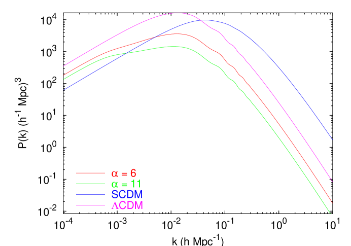
FIG. 6.: Matter power spectrum for the Ratra-Peebles potential for two values of $\alpha$, $\alpha=6$ (red curve) and $\alpha=11$ (green curve) and with cosmological parameters equal to $h=0.5$, $\Omega_{\mathrm{b}}=0.05$, $\Omega_{\mathrm{Q}}=0.7$, $\Omega_{\mathrm{c}dm}=1-\Omega_{\mathrm{b}}-\Omega_{\mathrm{Q}}$, $n_{\mathrm{S}}=0.99$, $A_{\mathrm{T}}=0$. The curves are compared with those obtained in the SCDM model (blue curve) and in the $\Lambda$CDM model (pink curve).

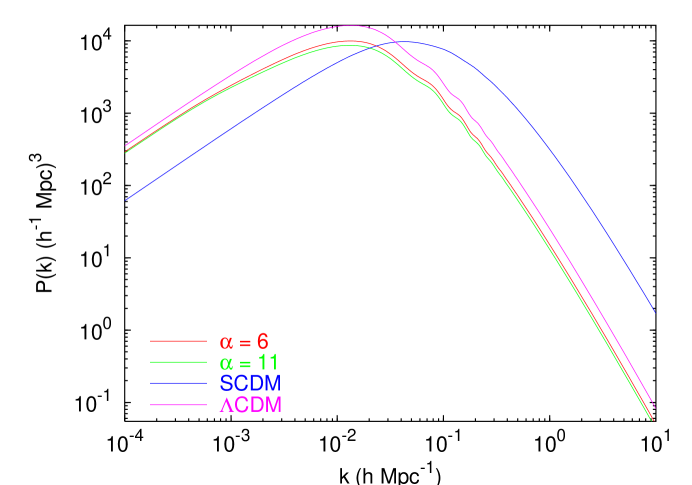
FIG. 7.: Matter power spectrum for the SUGRA potential for two values of $\alpha$, $\alpha=6$ (red curve) and $\alpha=11$ (green curve) and with cosmological parameters equal to $h=0.5$, $\Omega_{\mathrm{b}}=0.05$, $\Omega_{\mathrm{Q}}=0.7$, $\Omega_{\mathrm{c}dm}=1-\Omega_{\mathrm{b}}-\Omega_{\mathrm{Q}}$, $n_{\mathrm{S}}=0.99$, $A_{\mathrm{T}}=0$. The curves are compared with those obtained in the SCDM model (blue curve) and in the $\Lambda$CDM model (pink curve).

The matter power spectrum also depends on the nature of the dark energy component (cosmological constant or quintessence) but the difference between the cosmological constant scenario and a quintessence scenario is less important. The matter power spectrum shows a peak the location of which is given by the Hubble radius at equivalence. In the $\Lambda$CDM and QCDM scenarios, the peak is at the same location contrary to the sCDM case for which the peak is located at smaller scales. Also, in models with low matter content, the ratio $\Omega_{\mathrm{b}}/\Omega_{\mathrm{c}dm}$ is higher which results in the presence of smooth oscillations at small scales. As for the CMB anisotropy spectrum, the small scales are similar in the $\Lambda$CDM and QCDM scenarios and important differences only occur on larger scales which are more affected by the change in the cosmic equation of state.

Let us now study in more details and for more realistic values of the cosmological parameters, the position and the height of the first Doppler peak. We start with the location of the first peak (denoted in what follows by $l_{1}$) and we study it in the plane $(\Omega_{\mathrm{m}},h)$ with the following values of the other cosmological parameters: $h^{2}\Omega_{\mathrm{b}}=0.019$ (the value predicted by standard BBN), $\Omega_{\Lambda,{\mathrm{Q}}}=0.7$, $A_{\mathrm{T}}=0$ and $n_{\mathrm{S}}=0.99$. The case of the cosmological constant is displayed in Fig. 8, the case of the Ratra-Peebles QCDM model in Fig. 9 and the case of the SUGRA QCDM model in Fig. 10.

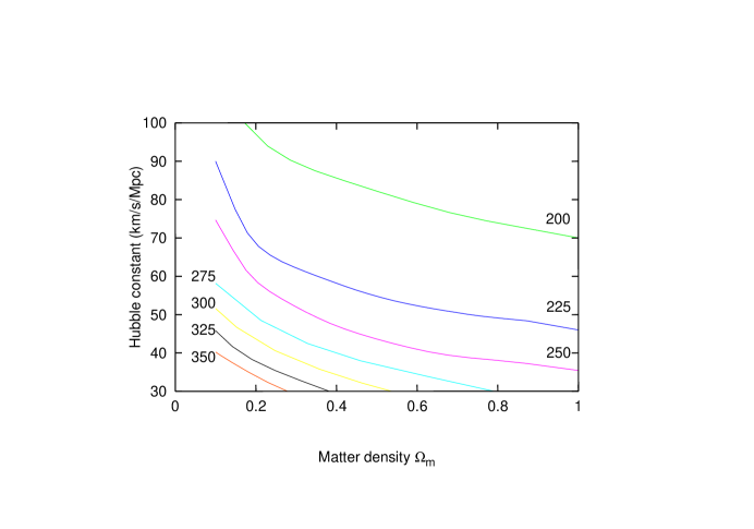
FIG. 8.: Contour plots of the first Doppler peak location in the $(\Omega_{\mathrm{m}},h)$ plane for the cosmological constant case. The other cosmological parameters are $h^{2}\Omega_{\mathrm{b}}=0.019$, $\Omega_{\Lambda}=0.7$, $A_{\mathrm{T}}=0$ and $n_{\mathrm{S}}=0.99$.

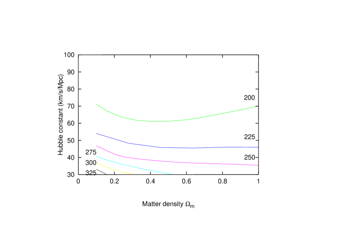
FIG. 9.: Contour plots of the first Doppler peak location in the $(\Omega_{\mathrm{m}},h)$ plane for the Ratra-Peebles QCDM case. The other cosmological parameters are $h^{2}\Omega_{\mathrm{b}}=0.019$, $\Omega_{\mathrm{Q}}=0.7$, $A_{\mathrm{T}}=0$ and $n_{\mathrm{S}}=0.99$.

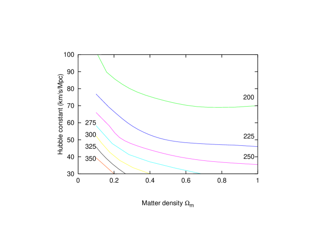
FIG. 10.: Contour plots of the first Doppler peak location in the $(\Omega_{\mathrm{m}},h)$ plane for the SUGRA QCDM case. The other cosmological parameters are $h^{2}\Omega_{\mathrm{b}}=0.019$, $\Omega_{\mathrm{Q}}=0.7$, $A_{\mathrm{T}}=0$ and $n_{\mathrm{S}}=0.99$.

These plots confirm the qualitative predictions made above and in particular the fact that, in general, $l_{1}^{\Lambda}>l_{1}^{\mathrm{S}UGRA}>l_{1}^{\mathrm{R}P}$. If one assumes that $\Omega_{\mathrm{m}}\simeq 0.3$ (since we have assumed $\Omega_{\Lambda}\simeq 0.7$) and $h\simeq 0.62$, this last value being consistent with the Hubble Space Telescope (HST) and SNIa measurements, then we obtain $l_{1}^{\Lambda}\simeq 225$, $l_{1}^{\mathrm{S}UGRA}\simeq 220$ and $l_{1}^{\mathrm{R}P}\simeq 200$. It is interesting to compare these values with the recent measurements of the first peak performed by BOOMERanG and MAXIMA-1. The BOOMERanG data indicate that $l_{1}=197\pm 6$ [20, 21] which is compatible with the Ratra-Peebles potential and a spatially flat Universe. On the other hand, the MAXIMA-1 data are consistent with a first peak located at $l_{1}\simeq 220$ [22, 23] which is, this time, in agreement with a cosmological constant or the SUGRA QCDM model.

Let us now study the height of the first Doppler peak. We study its variation in the plane $(\Omega_{\mathrm{b}},n_{\mathrm{S}})$ for the following values of the cosmological parameters: $h=0.62$, $\Omega_{\Lambda,{\mathrm{Q}}}=0.7$. The case of the $\Lambda$CDM model is displayed in Fig. 11 whereas the cases of the Ratra-Peebles QCDM and SUGRA QCDM are presented in Figs. 12 and 13, respectively.

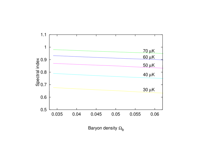
FIG. 11.: Contour plots of the height of the first peak in the $(\Omega_{\mathrm{b}},n_{\mathrm{S}})$ plane with $h=0.62$, $\Omega_{\Lambda}=0.7$ for the case of the $\Lambda$CDM model.

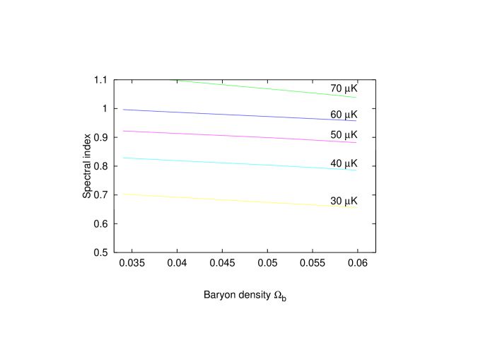
FIG. 12.: Contour plots of the height of the first peak in the $(\Omega_{\mathrm{b}},n_{\mathrm{S}})$ plane with $h=0.62$, $\Omega_{\mathrm{Q}}=0.7$ for the case of the Ratra-Peebles QCDM model.

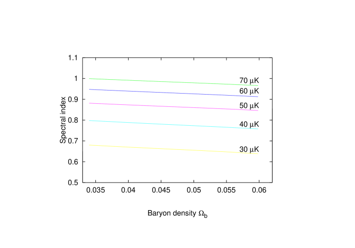
FIG. 13.: Contour plots of the height of the first peak in the $(\Omega_{\mathrm{b}},n_{\mathrm{S}})$ plane with $h=0.62$, $\Omega_{\mathrm{Q}}=0.7$ for the case of the SUGRA QCDM model.

We would like to emphasize that the importance of gravitational waves is crucial in this case. Indeed, as already mentioned, the presence of gravitational waves modifies the normalization and, as a consequence, the height of the peaks. The BOOMERanG data indicate that $\delta T_{200}\simeq 69\pm 8\,{\rm{\mu K}}$ [20, 21] whereas the MAXIMA-1 ones give $\delta T_{220}\simeq 78\pm 6\,{\rm{\mu K}}$ [22, 23], this discrepancy being possibly explained by problems in the calibration of these experiments. If we adopt the value $\Omega_{\mathrm{b}}\simeq 0.0595$, compatible with BBN, we see that, in the Ratra-Peebles QCDM model, a height of the first peak compatible with the BOOMERanG and MAXIMA-1 data leads to a value of the scalar spectral index such that $n_{\mathrm{S}}>1$. This is not compatible with standard inflation and cannot be realized with one scalar field. We interpret this as a new evidence that the Ratra-Peebles QCDM model (at least with this value of $\alpha$) is excluded by the observations. For the cases of $\Lambda$CDM and SUGRA QCDM, we learn from the previous plots that the spectral index must be very close to one.

We now turn to the study of the second Doppler peak. First of all, we should say something about the observational situation. With regards to the detection of a second peak, it is difficult to deduce something from the BOOMERanG data. The error bars are still large and the data are, for the moment, compatible with a second peak (with a height maybe smaller than predicted by standard inflation) but also with no peak at all, even if one can see a small rise of the signal at $l_{2}\simeq 550$ [20, 21]. Only $5\%$ of the data of this experimement have been analysed so far and one should wait for the rest of the data analysis to be completed. On the other hand, the MAXIMA-1 show “a suggestion of a peak at $l_{2}\simeq 525$” [22] the height of which would be $\delta T_{525}\simeq 48\,{\rm{\mu K}}$. One could even argue that the beginning of a third peak has been observed. In fact, considering all the uncertainties in such measurements, we are of the opinion that a reasonable attitute is simply to wait for more data. On the theoretical side, it was argued by Kamionkowski and Buchalter [40] that the location of the second peak can probe the dark energy density. The main idea is to study the contour plots of $l_{2}$ in the plane $(\Omega_{\mathrm{m}},h)$. Then, a measurement of $l_{2}$, knowing $h$ by other means , immediately determines the value of $\Omega_{\mathrm{m}}$. It was claimed in Ref. [40] that this strategy does not depend on whether the dark energy is a cosmological constant or a quintessence field. We show that this claim is not correct and that the nature of the dark energy matters. The contour plots of $l_{2}$ in the case of a cosmological constant are displayed in Fig. 14 for the cosmological parameters given by $h=0.62$, $\Omega_{\Lambda}=0.7$, $h^{2}\Omega_{\mathrm{b}}=0.019$, $n_{\mathrm{S}}=0.99$. These plots are in agreement with the results found in Ref. [40].

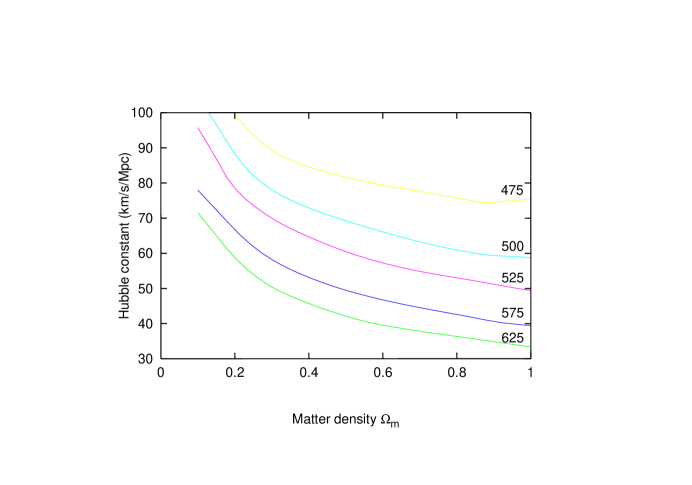
FIG. 14.: Contour plots of the location of the second peak in the $(\Omega_{\mathrm{m}},h)$ plane with $h=0.62$, $\Omega_{\Lambda}=0.7$, $h^{2}\Omega_{\mathrm{b}}=0.019$, $n_{\mathrm{S}}=0.99$ for the cosmological constant case.

The corresponding contour plots for the Ratra-Peebles and SUGRA CDM models are presented in Figs. 15 and 16. In addition, in order to show that there is indeed an important difference, we also display the contour plots for a cosmological constant which, for a given value of $l_{2}$, is always above the QCDM curve. The fact that there is a difference does not totally invalidate the idea of Ref. [40]. But it means that, in order to use it, we should first identify the physical nature of the dark energy, for example with a measurement of its equation of state parameter.

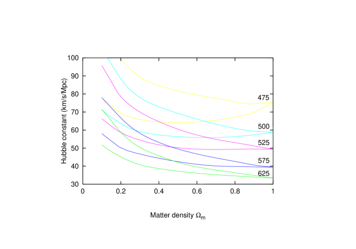
FIG. 15.: Contour plots of the location of the second peak in the $(\Omega_{\mathrm{m}},h)$ plane with $h=0.62$, $\Omega_{\Lambda,{\mathrm{Q}}}=0.7$, $h^{2}\Omega_{\mathrm{b}}=0.019$, $n_{\mathrm{S}}=0.99$ for the Ratra-Peebles QCDM model. The corresponding contour plots for the cosmological constant (upper curves) are also displayed for comparison.

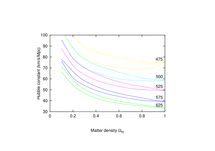
FIG. 16.: Contour plots of the location of the second peak in the $(\Omega_{\mathrm{m}},h)$ plane with $h=0.62$, $\Omega_{\Lambda,{\mathrm{Q}}}=0.7$, $h^{2}\Omega_{\mathrm{b}}=0.019$, $n_{\mathrm{S}}=0.99$ for the SUGRA QCDM model. The corresponding contour plots for the cosmological constant (upper curves) are also displayed for comparison.

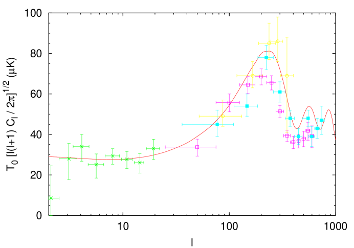
FIG. 17.: Band power $\delta T_{l}$ for the $\Lambda$CDM model with $h=0.62$, $\Omega_{\Lambda}=0.7$, $\Omega_{\mathrm{b}}=0.595$ and $n_{\mathrm{S}}=0.99$. The data point are those of the COBE, BOOMERanG, MAXIMA-1 and Saskatoon experiments.

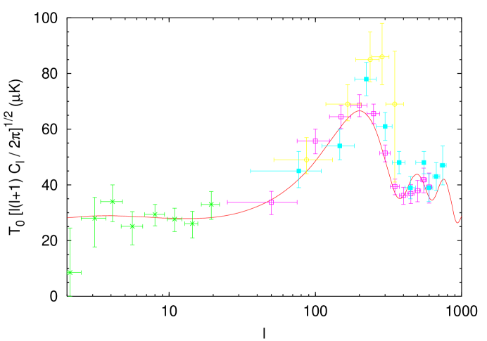
FIG. 18.: Band power $\delta T_{l}$ for the Ratra-Peebles QCDM model with $h=0.62$, $\Omega_{\mathrm{Q}}=0.7$, $\Omega_{\mathrm{b}}=0.0595$ and $n_{\mathrm{S}}=0.99$. The data point are those of the COBE, BOOMERanG, MAXIMA-1 and Saskatoon experiments.

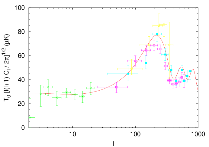
FIG. 19.: Band power $\delta T_{l}$ for the SUGRA QCDM model with $h=0.62$, $\Omega_{\mathrm{Q}}=0.7$, $\Omega_{\mathrm{b}}=0.0595$ and $n_{\mathrm{S}}=0.99$. The data point are those of the COBE, BOOMERanG, MAXIMA-1 and Saskatoon experiments.

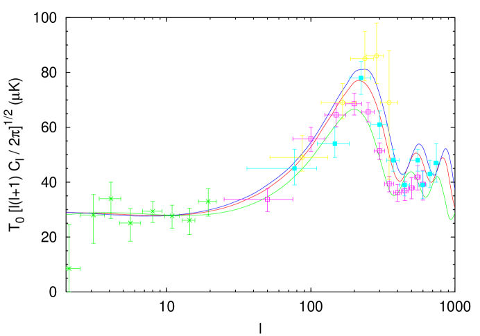
FIG. 20.: Band power $\delta T_{l}$ for the $\Lambda$CDM model (blue curve), Ratra-Peebles QCDM model (green curve) and the SUGRA QCDM model (red curve) with $h=0.62$, $\Omega_{\Lambda,{\mathrm{Q}}}=0.7$, $\Omega_{\mathrm{b}}=0.0595$ and $n_{\mathrm{S}}=0.99$. The data point are those of the COBE, BOOMERanG, MAXIMA-1 and Saskatoon experiments.

As for the first peak, we have $l_{2}^{\Lambda}>l_{2}^{\mathrm{S}UGRA}>l_{2}^{\mathrm{R}P}$. Roughly speaking, for $h\simeq 0.62$, $\Omega_{\mathrm{m}}\simeq 0.3$, we have $l_{2}^{\Lambda}\simeq 550$, $l_{2}^{\mathrm{S}UGRA}\simeq 525$ and $l_{2}^{\mathrm{R}P}\simeq 500$. Interestingly enough, the SUGRA QCDM model seems to predict the correct location of the “suggested second peak” [22], just in between the location predicted by the $\Lambda$CDM model and the Ratra-Peebles QCDM model. Of course, it is premature to conclude and only more data could allow to know whether this is indeed the case or whether this is just a coincidence.

Finally, we display the multipole moments for the $\Lambda$CDM model, the Ratra-Peebles QCDM model and the SUGRA QCDM model in Figs. 17, 18 and 19, respectively, for the following cosmological parameters (deduced from the previous considerations): $h=0.62$, $\Omega_{\Lambda}=0.7$, $\Omega_{\mathrm{b}}=0.0595$ and $n_{\mathrm{S}}=0.99$. The data points of COBE, BOOMERanG, MAXIMA-1 and Saskatoon have been added to the plots for comparison. These curves represent the predictions of each model and special attention must be paid to third peak which is certainly one of the next important experimental challenge. In Fig. 20, we present the three curves together in order to make the comparison easier. It should be emphasized again that the multipole moments predicted by the SUGRA QCDM model are unique in the sense that they do not depend on the free parameter in the potential. From these plots, we see that the SUGRA QCDM model is, among the three models studied here, the best fit of the MAXIMA-1 data. It is the only model for which the theoretical curve $\delta T$ versus $l$ goes through all the $1\sigma$ error bars of this experiment. However, we should be careful not to overestimate the relevance of this result since uncertainties are still large, for instance because the comparison of the calibrations of different experiments is always a difficult task. We should also keep in mind that $2\sigma$ deviations are always possible. Thus, we are waiting eagerly for the new data to see whether quintessence, and especially SUGRA quintessence, can confirm the hints of this article and fits the data better than the other QCDM models.

V conclusion

The quintessence scenario provides a general framework within which the issue of the energy density of the Universe can be tackled. In particular long-standing issues such as coincidence problem (and maybe the fine-tuning problem) receive reasonnable answers for a class of models possessing the property of tracking fields, i.e. the evolution of the quintessence field is driven at small redshift towards an attractor independently of the initial conditions. In the same spirit it seems very enticing to draw consequences of the quintessence hypothesis on other cosmological observables, the most prominent ones being the cosmological anisotropies. Recent measurement of the CMB anisotropies by the BOOMERanG and MAXIMA-1 experiments give a first indication on the location of the peaks in the CMB multipoles. It seems therefore topical to understand the consequence of the quintessence hypothesis on the CMB anisotropies.

In this paper we have confronted analytical methods with numerical results. Using the former we establish that the quintessence perturbation are independent of the initial conditions. This is confirmed by a full numerical computation. This allows us to study the CMB anisotropies. In particular we have paid particular attention to the comparison between three possible models: the cosmological constant model, the Ratra-Peebles and SUGRA quintessence models. We have also compared these three models with the existing data from the BOOMERanG and MAXIMA-1 experiments. As a rule the location of the first peak is shifted to the right for models having an equation of state $\omega$ closer to $-1$. This entails that the location of the first peak for the first peak of the MAXIMA-1 data is fitted by the SUGRA model. Similarly the location of the second peak around $l_{2}\simeq 525$ as suggested by MAXIMA-1 seem to indicate that the SUGRA model comes closer to be the best of these three models. One of the foreseeable challenges will be to carry out a thorough analysis of the forthcoming data in order to distinguish these three models even more clearly.

From the particle physics point of view most of the quintessence models discussed so far have neglected the crucial effects of SUSY breaking. It may well be that the effects of SUSY breaking, on top of necessitating a severe fine-tuning of the cosmological constant, will induce drastic modifications in the functional form of the quintessence potential. It is certainly a tantalizing challenge to include the effects of SUSY breaking within the supergravity models of quintessence [58]. On the other hand there exists the possibility that the cosmological constant problem will be resolved using ideas stemming from extra-dimension scenarios involving an effective supersymmetry in four dimensions [7]. The investigation of such models might well shed new light on the origin of the quintessence field.

As must be clear by now the issues raised by the cosmological constant problem, the quintessence scenario and its proper understanding within particle physics are many-fold. The experimental results which will be available in the near future might help in disentangling some of these very conspicuous matters.

REFERENCES

- [1] S. Perlmutter et al, Nature391, 51 (1998); S. Perlmutter et al, ApJ517, 565 (1999); P.M. Garnavich et al, ApJ493, L53 (1998); A.G. Riess et al, Astron. J. 116, 1009 (1998).
- [2] B. Ratra and P.J.E. Peebles, Phys. Rev. D37, 3406 (1988).
- [3] P.G. Ferreira and M. Joyce, Phys. Rev. D58, 023503 (1998).
- [4] I. Zlatev, L. Wang and P.J. Steinhardt, Phys. Rev. Lett.82, 896 (1999). Preprint astro-ph/9807002.
- [5] P.J. Steinhardt, L. Wang and I. Zlatev, Phys. Rev. D59, 123504 (1999). Preprint astro-ph/9812313.
- [6] S. Weinberg, Rev. Mod. Phys. 61, 1 (1989).
- [7] E. Witten, preprint hep-ph/0002297.
- [8] P. Binétruy, Phys. Rev. D60, 063502 (1999). Preprint hep-ph/9810553.
- [9] A. de la Macorra, preprint hep-ph/9910330.
- [10] P. Brax and J. Martin, Phys. Rev. D61, 103502 (2000). Preprint astro-ph/9912046.
- [11] P. Brax and J. Martin, Phys. Lett. 468B, 40 (1999). Preprint astro-ph/9905040.
- [12] S. Carroll, Phys. Rev. Lett.81, 3067 (1998).
- [13] T. Chiba, Phys. Rev. D60, 083508 (1999).
- [14] J.–P. Uzan, Phys. Rev. D59, 123520 (1999).
- [15] L. Amendola, Phys. Rev. D60, 043501 (1999).
- [16] A. Riazuelo and J.–P. Uzan, submitted to Phys. Rev. D. Preprint astro-ph/0004156.
- [17] P.J.E. Peebles and A. Vilenkin, Phys. Rev. D59, 063505 (1999).
- [18] M. Giovannini, Class. Quant. Grav. 16, 2905 (1999); Phys. Rev. D 60, 123511 (2000).
- [19] http://oberon.roma1.infn.it/boomerang/
- [20] P. de Bernardis et al, Nature404, 955 (2000).
- [21] A.E. Lange et al, preprint astro-ph/0005004.
- [22] S. Hanany et al, preprint astro-ph/0005123.
- [23] A. Balbi et al, preprint astro-ph/0005124.
- [24] http://map.gsfc.nasa.gov/
- [25] http://astro.estec.esa.nl/Planck/
- [26] http://astro.uchicago.edu/home/web/sdss/www/
- [27] M. Tegmark, ApJ514, L69 (1999).
- [28] I. Zehavi and A. Dekel, Nature401, 252 (1999). Preprint astro-ph/9904221.
- [29] L. Wang, R.R. Caldwell, J.P. Ostriker and P.J. Steinhardt, ApJ530, 17 (2000). Preprint astro-ph/9901388.
- [30] I. Waga and J.A. Frieman, preprint astro-ph/0001354.
- [31] S. Perlmutter, M.S. Turner and M. White, Phys. Rev. Lett.83, 670 (1999). Preprint astro-ph/9901052.
- [32] A.R. Cooray and D. Huterer, ApJ513, L95 (1999). Preprint astro-ph/9901097.
- [33] G. Efstathiou, MNRAS 310, 842 (2000). Preprint astro-ph/9904356.
- [34] R.R. Caldwell, R. Dave and P.J. Steinhardt, Phys. Rev. Lett.80, 1582 (1998).
- [35] P.G. Ferreira and M. Joyce, Phys. Rev. Lett.79, 4740 (1997).
- [36] C. Baccigalupi and F. Perrotta, preprint astro-ph/9811385.
- [37] F. Perrotta, C. Baccigalupi and S. Matarrese, Phys. Rev. D61, 023507 (2000). Preprint astro-ph/9906066.
- [38] C. Ma, R.R. Caldwell, P. Bode and L. Wang, ApJ521, L1 (1999). Preprint astro-ph/9906174.
- [39] S. Dodelson, M. Kaplinghat and E. Stewart, preprint astro-ph/0002360.
- [40] M. Kamionkowski and A. Buchalter, preprint astro-ph/0001045.
- [41] J. Martin and D.J. Schwarz, Phys. Rev. D57, 3302 (1998).
- [42] R.A. Battye, M. Bucher and D. Spergel, preprint astrop-ph/9908047.
- [43] V. Sahni and L. Wang, preprint astro-ph/9910097.
- [44] T. Barreiro, E.J. Copeland and N.J. Nunes, Phys. Rev. D61, 127301 (2000). Preprint astro-ph/9910214.
- [45] A. Albrecht and C. Skordis, Phys. Rev. Lett.84, 2076 (2000). Preprint astro-ph/9908085.
- [46] J.E. Kim, JHEP 9905, 022 (1999). Preprint hep-ph/9811509.
- [47] S.M. Carroll, Phys. Rev. Lett.81, 3067 (1998). Preprint astro-ph/9806099.
- [48] C. Kolda and D.H. Lyth, Phys. Lett. 458B, 197 (1999). Preprint hep-ph/9811375.
- [49] J.C. Fabris and J. Martin, Phys. Rev. D55, 5205 (1997).
- [50] L.P. Grishchuk, Phys. Rev. D50, 7154 (1994).
- [51] P.J.E. Peebles, The large scale structure of the Universe (Princeton University Press, Princeton, 1980).
- [52] R.K. Sachs and A.M. Wolfe, ApJ147, 73 (1967).
- [53] G.F. Smoot et al, ApJ396, L1 (1992); C.L. Bennett et al, ApJ464, L1 (1996).
- [54] K.A. Olive, G. Steigman and T.P.Walker, preprint astro-ph/9905320.
- [55] K.M. Nollett and S. Burles, Phys. Rev. D61, 123505 (2000). Preprint astro-ph/0001440.
- [56] C.B. Netterfield et al, ApJ474, 47 (1997); E. Wollack et al, ApJ476, 440 (1997).
- [57] W. Hu, in The universe at high-, large scale structure and the cosmic microwave background, edited by E. Martinez-Gonzalez and J.L. Sanz, p. 207 (Springer Verlag, Berlin, Germany, 1996).
- [58] P. Brax, J. Martin and A. Riazuelo, in preparation.