Is MS1054-03 an exceptional cluster? A new investigation of ROSAT/HRI X-ray data

Abstract

We reanalyzed the ROSAT/HRI observation of MS1054-03, optimizing the channel HRI selection and including a new exposure of 68 ksec. From a wavelet analysis of the HRI image we identify the main cluster component and find evidence for substructure in the west, which might either be a group of galaxies falling onto the cluster or a foreground source.

Our 1–D and 2–D analysis of the data show that the cluster can be fitted well by a classical $\beta$–model centered only $20\arcsec$ away from the central cD galaxy. The core radius and $\beta$ values derived from the spherical model($\beta=0.96_{-0.22}^{+0.48}$) and the elliptical model ($\beta=0.73\pm 0.18$) are consistent.

We derived the gas mass and total mass of the cluster from the $\beta$–model fit and the previously published ASCA temperature ($12.3^{+3.1}_{-2.2}{\rm\ keV}$). The gas mass fraction at the virial radius is $\hbox{$f_{gas}$}=(14\small{[-3,+2.5]}\pm 3\ )\%$ for $\Omega_{0}=1$, where the errors in brackets come from the uncertainty on the temperature and the remaining errors from the HRI imaging data. The gas mass fraction computed for the best fit ASCA temperature is significantly lower than found for nearby hot clusters, $\hbox{$f_{gas}$}=20.1\ \pm 1.6\ \%$. This local value can be matched if the actual virial temperature of MS1054-032 were close to the lower ASCA limit ($\sim 10~{}{\rm\ keV}$) with an even lower value of $8~{}{\rm\ keV}$ giving the best agreement. Such a bias between the virial and measured temperature could be due to the presence of shock waves in the intracluster medium stemming from recent mergers. Another possibility, that reconciles a high temperature with the local gas mass fraction, is the existence of a non zero cosmological constant.

1. Introduction

MS1054-03 is the most distant cluster of galaxies found in the X-ray selected sample of the Einstein Extended Medium Sensitivity Survey (EMSS; Gioia et al., 1990). Due to the extreme sensitivity of the high–mass end of the cluster mass function to the density parameter, $\Omega_{0}$, the existence of massive, virialized clusters at high z is of great cosmological significance (e.g. Oukbir & Blanchard 1992). The very existence of even a few massive clusters at redshifts approaching unity and beyond strongly argue against cosmological models with $\Omega_{0}=1$.

There is a general consensus that MS1054-03 is such a massive cluster, based on its high X-ray temperature, $kT=12.3^{+3.1}_{-2.2}$ keV, measured with ASCA (Donahue et al. 1998 hereafter D98), its high velocity dispersion (Tran et al. 1999) and intense weak lensing signal (Luppino & Kaiser 1997). On the other hand its apparent complex morphology (D98) might indicate that MS1054-03 has not yet reached an equilibrium state, which could cast some doubt on the dynamical mass estimates and on the relevance of the cluster for cosmological tests. Tran et al. (1999) emphasized the good agreement between the various mass estimates, but the large error bars must be noted.

In this paper we re-investigate the ROSAT/HRI observations of MS1054, including a new exposure taken in 1997. We first try to better understand the cluster morphology. A wavelet analysis of the HRI image is performed to unravel significant substructures and identify the main cluster component. A $\beta$–model is then fitted to the data. From the fit results, we estimate for the first time the gas mass of this cluster. A comparison of the gas mass fraction of MS1054-032, with the gas mass fraction of nearby clusters, provides a consistency check on the total mass estimate, assuming that the gas mass fraction in clusters does not evolve with redshift.

Throughout the paper we assume $H_{0}=50$ km/sec/Mpc, $q_{0}=0.5$, $\Lambda=0$ and all quoted error bars are 1 $\sigma$ unless otherwise stated. At the redshift of the cluster, $z=0.83$, one arcmin corresponds to $497{\rm h}_{50}^{-1}$ kpc.

2. Observations

MS1054-03 was observed by the ROSAT HRI (Trümper 1992) for 190,754 sec in total: an exposure of $\sim 122$ ksec in 1996, which was analyzed and presented in D98 and a pointing of 68 ksec taken in 1997. In this analysis we combined the exposures of 1996 and 1997 and we selected only HRI channels 1 to 7 (David et al. 1997) in order to maximize the signal-to-noise ratio. The background level is thus lowered by a factor of about 2. The HRI image smoothed with a Gauss filter is shown on Fig. 1 and looks similar to the image presented by D98.

3. Morphology

In order to remove noise and to identify the significant structures we performed a wavelet-analysis of the HRI raw image with the Multi-scale Vision Model (MVM) package (Rué & Bijaoui 1997). We explicitly took into account the Poisson statistics and the significance level was set to $3\sigma$. The algorithm is optimized for the detection of diffuse components by normalizing the wavelet coefficients by their energy (Rué & Bijaoui 1997, Arnaud et al. 2000).

The reconstructed image consists of point sources and one large scale diffuse component at the cluster position. To extract possible substructures, we reapplied the multi-scale analysis to the reconstructed diffuse source only. Two components are detected that are shown in Fig. 2, superimposed on the cluster optical image. The main component ($\sim 90\%$ of the flux) is centered at RA = $10^{h}56^{m}58.47^{s}$, Dec.= $-03\deg 37\arcmin 31.2\arcsec$, about $20~{}\arcsec$ ($166~{}{\rm h}_{50}^{-1}$ kpc) from the dominant galaxy (D98). We identify this structure with the main cluster component. It is very elliptical with an elongation in the east-west direction. The orientation follows the filamentary structure found in the optical and in the weak lensing map (Luppino & Kaiser 1997). The second component is compact and lies in the west, with an offset of 0.6 arcmin with respect to the main cluster center. It coincides with the brightest image peak, identified by D98, but its reconstructed flux is only $\sim 10\%$ of the main cluster flux.

This western source might be a subcluster gravitationally connected to the main cluster, or a projection effect due to a group of galaxies in the field-of-view (FOV) or even a point source. The available data are insufficient to settle this issue. There is a weak indication that the source is extended, from our comparison of the source surface brightness profile with the point spread function (PSF) of the ROSAT/HRI (David et al. 1997). However, due to the lack of bright sources in the FOV, we cannot correct for possible alignment uncertainties, and the extent might be due to errors in the aspect reconstruction or residual main cluster emission. Very close to the maximum of this source we find several cluster members so this structure might be a subgroup falling right onto the cluster. Finally it must be noticed that the reconstructed surface mass density by Luppino & Kaiser (1997) presents an extension in the west. Although it is unresolved, it might indicate that the western X–ray component does trace a gravitational potential.

4. Isothermal beta-model fits

We performed $\beta$-model fits to the data using spherically symmetric (1–D) and elliptical (2–D) $\beta$–model fits. We excluded from the fits circular regions corresponding to serendipitous point sources. In the 1–D case the X-ray surface brightness profile is given by:

$$S=S_{0}\left(1+r^{2}/r_{c}^{2}\right)^{-3\beta+0.5}+B$$ (1)

where $r_{c}$ is the core radius, $\beta$ is a slope parameter and $B$ is the background level. The functional form for the elliptical $\beta$–model can be found in Neumann & Böhringer (1997).

4.1. Spherical model

We binned the data in concentric annuli with the center at the position determined from the above wavelet reconstruction. The $\beta$–model was convolved with the PSF of the ROSAT/HRI. The free parameters in the fit are $S_{0}$, $r_{c}$, $\beta$ and $B$. We first consider the main cluster component in a common way by excluding non-symmetric features in the data, i.e. a circular region around the substructure in the west. Fig. 3 shows the observed surface brightness profile and the best fit model. The reduced $\chi^{2}$ value is $\chi^{2}=0.97$, and the shape parameters are well constrained (see Tab.1). On the other hand if the substructure is not removed, a good fit is still obtained ($\chi^{2}=0.99$) but the best fit shape parameters are unreasonably large ($\beta=2.,r_{c}=840~{}{\rm kpc}$), and poorly constrained ($\beta>1.1$). An artificial increase of the best fit shape parameters is a well known effect of not excising a secondary sub-cluster in the $\beta$–model fit (Jones & Forman 1999). A good fit is still obtained due to the large errors on the observed profile, whereas no upper limit on $\beta$ can be set because the best fit core radius becomes similar to the maximum radius of cluster emission detected.

4.2. Elliptical model

We also fitted an elliptical isothermal $\beta$–model to the HRI image. Again we excise the substructure in the west as well as other weak unresovled sources in the FOV. Due to the limited statistics of the observation, we did not attempt to fit the whole image with a $\beta$–model and an additional component for the substructure, since the elliptical $\beta$–model has already 8 fit parameters.

The iso-contours of the best fit model are superimposed on the cluster image in Fig. 1. The fitting procedure is described in full detail in Neumann (1999). We binned the data into an image with a pixel size of $5\arcsec\times 5\arcsec$. The fit included all pixels less than 4.6 arcmin away from the central pointing position of $10^{h}57^{m}00.00^{s}$, and Dec.= $-03\deg 37\arcmin 12.0\arcsec$ (J2000). The central position of the cluster was left free to vary.

As we are dealing with low number statistics in each image pixel, which shows non-Gaussian behavior, we smoothed the data with a Gauss filter ($\sigma=10\arcsec$) before fitting. The modeling accounts for the Gauss filtering and for the PSF (the fitted model is convolved with the Gauss filtered PSF). To calculate the errors of the $\beta$–model parameters we performed a Monte-Carlo analysis in which we added Poisson noise to the data and fitted the $\beta$–model subsequently. We performed 100 Monte-Carlo realizations.

The validity of this approach was discussed in Neumann & Böhringer (1997) and Neumann (1999). In order to see whether it is still free of systematics in this regime of extremely low signal-to-noise data (the central cluster intensity is only a factor of two higher than the background level) we simulated 100 realizations of the image of the best fit $\beta$–model cluster including background. The Poisson statistics were defined according to the length of the actual exposure time. We subsequently fitted a $\beta$–model to these artificial smoothed images, as for the real image. The results are satisfactory, as the mean output values are practically identical to the input values, with differences much smaller than the actual determined error bars for MS1054-03. The width of their distribution is slightly smaller than the errors determined from the real data.

4.3. Comparison of the 1–D and 2–D models

The values of the spherical and elliptical $\beta$–model parameters for the main cluster component together with their 1 $\sigma$ errors are given in Tab.1 and the two $\beta$–models profiles are plotted on Fig. 3. The best fit center of the elliptical model is only $5~{}\arcsec$ away from the central position from the wavelet analysis, which we also choose as the center for the 1–D fit. As already mentioned, these central positions are also in excellent agreement with the position of the brightest cluster member. The 1–D and 2–D best fit parameters are consistent. The background level is slightly higher in the 1–D fit which explains the lower central value and the higher value for $\beta$. Nevertheless the $68\%$ confidence intervals for the fitted shape parameters show a large large region of overlap.

5. Luminosity

The background estimated from the 1–D model fit was subtracted from the radial profile. An additional $5\%$ systematic uncertainty was assumed on its level. The cluster emission is detected up to $2\arcmin$ or $1~{}{\rm h}_{50}^{-1}~{}{\rm Mpc}$ at the $68\%$ confidence level. The observed count rate within this aperture is $(9\pm 2)\times 10^{-3}$ cts/s, $\sim 25\%$ higher than the value given by D98 (subtracting additional sources, including the western structure for consistency). We recall that the count rate of the western substructure is only $10\%$ of the cluster flux. The count rates derived from the best fit 2–D model is consistent but higher $11\times~{}10^{-3}$cts/s, a consequence of the lower best fit background, in this case.

The observed count rate was translated into luminosity, assuming a cluster temperature of 12.3 keV, as measured by D98 from ASCA data. The derived X–ray luminosity is $L_{\rm X}=1.2\times 10^{45}{\rm h}_{50}^{-2}$ ergs/s (0.1–2.4 keV rest frame). The bolometric luminosity within $2\arcmin$ in radius, $L_{\rm bol}=4.3\pm 0.9\times 10^{45}{\rm h}_{50}^{-2}$ergs/s, is consistent with the ASCA value of $4.4\times 10^{45}{\rm h}_{50}^{-2}$ergs/s (D98). This might be fortuitous though since the later includes all components in the field. The bolometric luminosity is lower than the value expected from the $L_{\rm X}$–$T$ relation of Arnaud & Evrard (1999), assuming this relation does not evolve with redshift. For a cluster with $T=12.3^{+3.1}_{-2.2}$ keV this correlation predicts a luminosity of $9.1^{+8.2}_{-4.0}\times 10^{45}~{}{\rm h}_{50}^{-2}$ergs/s. Up to now it is not clear whether the $L_{\rm X}$–$T$ relation evolves with redshift or not (see for example Schindler 1999). Also, the total X-ray luminosity of MS1054 might be actually higher since the cluster might extend beyond the radius of detection. However, due to the low S/N ratio of this observation such extrapolation is very sensitive to the assumed background level and $\beta$ parameter.

6. Mass content

6.1. Mass estimates

The cluster gas mass profile $M_{\rm gas}(r)$ can be derived from the best fit $\beta$–model , given the observed temperature and $N_{H}$ values. As the emissivity in the ROSAT/HRI energy band is nearly insensitive to the temperature, the uncertainty on the gas mass is overwhelmingly dominated by the errors on the $\beta$–model parameters. The association of the western source with the cluster is unclear. However, in practice, this additional uncertainty has no significant impact on the gas mass estimate. If the substructure is included in the $\beta$–model analysis, the derived gas mass differs by less than $5\%$ from the value obtained when excising it; the derived mass is increased within the detection radius (as a consequence of the $\sim 10\%$ higher flux) and artificially decreased when one extrapolates the data to higher radii (due to the higher derived $\beta$ value). In the following we only consider the main cluster component and its corresponding $\beta$ model.

The total mass can be estimated with the isothermal $\beta$–model approach (BM), which is thought to be roughly valid even if the cluster is not fully in hydrostatic equilibrium (e.g Schindler 1996). The alternative is to employ the virial theorem (VT) at given density contrast, over the mean mass density of the Universe at the cluster redshift, normalized from numerical simulations (Evrard et al. 1996). The resulting $M$–$T$ relation (see Appendix) depends both on redshift and on the cosmological parameters $\Omega_{0}$ and $\Lambda$ (Voit & Donahue 1998). We used the analytical expression from Bryan & Norman (1998).

We first fix the temperature to the best fit ASCA value of k$T=12.3~{}{\rm\ keV}$ and consider an $\Omega_{0}=1$ Universe. The uncertainty introduced by the errors on the temperature is discussed later. The statistical errors on $M_{\rm gas}(r)$ and on $M_{\rm BM}(r)$ due to the uncertainties in the $\beta$–model , are estimated following the general method described in Elbaz et al. (1995). The derived mass profiles are plotted in Fig. 4. Tab.2 summarizes the mass estimates at $1~{}{\rm h}_{50}^{-1}~{}{\rm Mpc}$ (the maximum radius of detection) and $1.65~{}{\rm h}_{50}^{-1}~{}{\rm Mpc}$ (the virial radius $R_{\rm V}$ for z=0.83 and k$T=12.3~{}{\rm\ keV}$ using the Evrard et al. (1996) simulations).

The 2–D model gas mass at $1~{}{\rm h}_{50}^{-1}~{}{\rm Mpc}$ is $15\%$ higher than the value derived from the 1–D model. This discrepancy, larger than the formal statistical uncertainties, is essentially due to the systematic difference in the background estimates, which dominates the error. As the derived $\beta$ value is consistently smaller in the 2–D fit, this discrepancy is amplified for extrapolated gas masses. It reaches $25\%$ at the virial radius. Similarly the total BM mass estimate which scales as $\beta$ is smaller for the 2–D model than for the 1–D model. Both are consistent with the VT estimate, which we will adopt in the following discussion. The gas mass is taken as the average of the 1–D and 2–D estimates. Their difference is an estimate of the systematic uncertainties that we add in quadrature to statistical ones. The gas mass fraction at the virial radius is thus $\hbox{$f_{gas}$}=14\pm 3\%$, for k$T=12.3~{}{\rm\ keV}$ and $\Omega_{0}=1$, the error coming from the uncertainty on the gas mass from the imaging data.

We performed the same analysis for the extreme values of the temperature, as allowed by the ASCA data at the $90\%$ confidence level (D98). For the lower limit on the temperature, k$T=10.1~{}{\rm\ keV}$, the virial radius is $1.58~{}{\rm Mpc}$ and the gas mass fraction within that radius is $\hbox{$f_{gas}$}=16.5\pm 3\%$. For k$T=15.4~{}{\rm\ keV}$, we get $R_{\rm V}=1.95~{}{\rm Mpc}$ and $\hbox{$f_{gas}$}=11\pm 3\%$.

In summary the gas mass fraction at the virial radius is $\hbox{$f_{gas}$}=14\small{[-3,+2.5]}\pm 3\ \%$ for $\Omega_{0}=1$. We have separated the uncertainties due to the errors on the temperature (in bracket), which affect essentially the total mass estimate, and the uncertainties from the imaging data, which only affect the gas mass estimate.

6.2. Comparison with nearby clusters

As mentioned above, a precise determination of the total mass of distant luminous clusters like MS1054-03 is crucial for the determination of $\Omega_{0}$ based on cluster abundances at high redshifts. Unfortunately there are still important uncertainties on the total mass estimate: statistical errors due to the errors on the temperature measurement but also possible systematic errors if the temperature is a biased estimator of the cluster mass. In particular the gas temperature might differ from the true virial temperature if the cluster were not in hydrostatic equilibrium.

By considering the additional information on the gas mass, we can however perform a consistency check on the total mass estimate. From a study of the intrinsic dispersion in the $L_{\rm X}$–$T$ relation, Arnaud & Evrard (1999) showed that the fractional variations of $f_{gas}$ at fixed cluster mass is very small. Since it is unlikely that the gas mass fraction evolves with redshift, the derived gas mass fraction of MS1054-03 should be consistent with the typical value of hot nearby clusters.

As a reference we first consider the best fit ASCA temperature (k$T=12.3~{}{\rm\ keV}$) and a $\Omega_{0}=1$ universe. The corresponding gas mass fraction of MS1054-03 is significantly smaller (at the 95$\%$ confidence level) than the value found by Arnaud & Evrard (1999) for hot nearby clusters, $\hbox{$f_{gas}$}=20.1\pm 1.6\ \%$. Obviously MS1054-03 might be a true outlier. Such outliers are rare but some, such as A1060, a cluster of exceptional low gas content in the local Universe (Arnaud & Evrard 1999), do exist. If this is not the case for MS1054, the low derived $f_{gas}$ value suggests that the actual virial temperature is lower than $12.3~{}{\rm\ keV}$ and/or that the adopted cosmology is wrong. We examine each possibility in turn.

The derived gas mass fraction depends on the assumed values of the cosmological parameters $\Omega_{0}$ and $\Lambda$. In the BM approach, $\hbox{$f_{gas}$}\propto d_{\rm A}^{3/2}$, where $d_{\rm A}$ is the angular distance (Pen 1997). In the VT approach adopted here the dependence of $f_{gas}$ is slightly different. $f_{gas}$ is both dependent on the geometry factor (the variation of $d_{\rm A}$) and on the normalization of the $M_{\rm V}({\rm or}R_{\rm V})$–$T$ relation. A detailed derivation of this dependence and necessary equations to compute the variation of $f_{gas}$ with $\Omega_{0}$ are given in the Appendix. The variation of the gas mass fraction of MS1054-03 with $\Omega_{0}$ is plotted on Fig. 5 for an open Universe ( $\Omega<1$, $\Lambda=0$) and a flat Universe ($\Omega_{0}+\Lambda=1$). For the best 1–D(2–D) $\beta$–model , the estimated gas mass fraction of MS1054-03 would be a factor of 1.2(1.3) larger if $\Omega_{0}=0.3$, $\Lambda=0.0$ and 1.4(1.5) times larger if $\Omega_{0}=0.3$,$\Lambda=0.7$. The gas mass fraction of MS1054-03 would in the later case be perfectly consistent with the local value, which would itself remain essentially unchanged ($<5\%$ increase).

The second possibility is that the virial temperature, and thus the virial mass, are smaller than given by the best fit ASCA value. The lower limit on the ASCA temperature (k$T=10.1~{}{\rm\ keV}$) yields a gas mass fraction marginally consistent with the local value. If the virial temperature were actually even somewhat lower, k$T=8~{}{\rm\ keV}$, the virial mass would decrease to $0.84\times 10^{15}\hbox{${\rm M}_{\sun}$}$, the virial radius to 1.3 Mpc and the gas mass within that radius, $1.7\times 10^{15}~{}\hbox{${\rm M}_{\sun}$}$, would reach $20\%$ of the virial mass and be a perfect match with the local value. A virial temperature of $8{\rm\ keV}$ is formally excluded by ASCA measurements at the $90\%$ confidence level but would be in better agreement with the measured velocity dispersion of $\sigma=1170\pm 150$ kms/s (Tran et al. 1999). In that case MS1054-03 would fit perfectly in the $\sigma-T$ relation established for $z=0.19-0.55$ clusters and the virial relation (Fig. 3 of Tran et al. 1999). The temperature would also be more consistent with the measured bolometric luminosity. A possible explanation for the measured temperature being significantly higher than the virial temperature (apart from contamination by a hard source like an absorbed AGN) would be the presence of shock waves in the gas if the cluster were indeed undergoing a recent merger.

7. Conclusion

Our wavelet analysis finds evidence for two components in the X–ray image of MS1054-03: a main diffuse component, with emission peaking at $20\arcsec$ from the brightest cluster member, and a compact substructure in the west, which coincides with the X-ray maximum in the ROSAT image. We emphasize that this brightest peak is not the centroid of the cluster. Indeed, when the western structure is excluded, the cluster emission is fitted well by a classical $\beta$–model , centered within $20\arcsec$ of the central cD galaxy. This indicates that we are then identifying the main cluster component.

Unlike previous attempts (D98, Ebeling et al. 1999), we obtained a good fit to the data with a $\beta$–model (low $\chi^{2}$ value) and derived well constrained parameters. This is a natural consequence of the higher S/N ratio of our data (optimum channel selection and longer exposure time) and our identification and removal of the western structure from our fits.

There are indications from the X–ray data that the cluster is not fully relaxed. The core radius ($\sim 400$ kpc) and ellipticity are relatively high and the western substructure could be an in-falling group. This is not unusual, such mergers do exist in the nearby Universe. Actually MS1054-03 appears very similar to A521 at z=0.27 (Arnaud et al. 2000), where the brightest peak is also associated with the subcluster.

The gas mass fraction derived for the best fit ASCA temperature of k$T=12.3~{}{\rm\ keV}$ is only consistent with the local value if $\Omega_{0}<1$, a flat $\Lambda$–dominated Universe being favored. The local value can be matched as well for $\Omega_{0}=1$, provided that the actual virial temperature is close to the lower ASCA limit ($\sim 10~{}{\rm\ keV}$), with an even lower value of $8~{}{\rm\ keV}$ giving the best match. To decide between the two options requires a systematic analysis of a large sample of distant clusters. MS1054-03 would appear as an outlier in the second case (low virial temperature) and not in the first case (flat $\Lambda$ dominated Universe). If the cluster’s actual mass is indeed lower than previously estimated, this might have consequences for the measurements of $\Omega_{0}$ based on the abundance of massive clusters at high redshift.

Finally we want to stress that the current data allow us to constrain the physics of MS1054 only with large error bars. Therefore better data, in particular spectroscopic data from Chandra and XMM, are strongly needed.

APPENDIX

In this Appendix we consider the gas mass fraction derived from X-ray data in the VT approach (see Sect.6.1) and examine how it depends on the assumed cosmological parameters, $\Omega_{0}$ and $\Lambda$.

The total mass $M_{\rm V}$ is estimated from the measured temperature and the mass-temperature relation derived from the virial theorem at given density contrast:

$$M_{\rm V}\propto\left(\frac{\Delta_{\rm c}(\Omega(z),\Lambda)\Omega_{0}}{\Omega(z)}\right)^{-1/2}\ (1+z)^{-3/2}\ \left({\rm k}T\right)^{3/2}$$ (1)

It depends on $\Omega_{0}$ and $\Lambda$, via the density contrast, $\Delta_{\rm c}(\Omega(z),\Lambda)$, and the density parameter of the universe at redshift z, $\Omega(z)$. The analytical expression of $\Delta_{c}$ and $\Lambda(z)$ can be found in Bryan & Norman (1998). The corresponding virial radius scales as:

$$R_{\rm V}\propto\left(\frac{\Delta_{\rm c}(\Omega(z),\Lambda)\Omega_{0}}{\Omega(z)}\right)^{-1/2}\ (1+z)^{-3/2}\ \left({\rm k}T\right)^{1/2}$$ (2)

We assume that the gas density $n_{\rm g}(r)$, follows a $\beta$–model: $n_{\rm g}(r)=n_{\rm g,0}\left[1+(r/r_{\rm c})^{2}\right]^{-3\beta/2}$. X-ray imaging data provides the central surface brightness $S_{0}$, the slope parameter $\beta$ and the angular core radius $\theta_{c}=r_{\rm c}/d_{\rm A}$, where $d_{A}$ is the angular distance.

The emission measure along the line of sight through the cluster center can be derived from $S_{0}$, independently of any cosmological parameters :

$$EM_{0}=\frac{4~{}\pi~{}(1+z)^{4}~{}S_{0}}{\Lambda(T,z)}$$ (3)

where $\Lambda(T,z)$ is the emissivity in the detector band, taking into account the interstellar absorption and the instrument spectral response.

Assuming that the X-ray atmosphere extends up to the virial radius, the central emission measure along the line of sight is linked to the gas density by $EM_{0}\propto\int_{0}^{R_{\rm V}}n_{\rm g}^{2}(r)~{}dr$, whereas the gas mass within $R_{V}$ is $M_{\rm gas}\propto\int_{0}^{R_{\rm V}}n_{\rm g}(r)~{}r^{2}~{}dr$. By combining the two expressions, we can derive an expression for the gas mass that varies as:

$$M_{\rm gas}\alpha R_{\rm V}^{5/2}\sqrt{EM_{0}}~{}Q(\beta,x_{\rm c})$$ (4)

where we have introduced the form factor $Q(\beta,x_{\rm c})=\langle{n_{\rm g}}\rangle/\sqrt{\langle{n_{\rm g}^{2}}\rangle_{los}}$. Here $\langle{n_{\rm g}}\rangle$ is the average gas density within $R_{\rm V}$ and $\langle{n_{\rm g}^{2}}\rangle_{los}$ is the average along the line–of–sight passing through the cluster center. For the $\beta$–model, this form factor depends on $\beta$ and the scaled core radius $x_{c}=r_{c}/R_{V}$:

$$Q(\beta,x_{\rm c}) = \frac{3\int_{0}^{1}\left[1+(x/x_{c})^{2}\right]^{-3\beta/2}~{}x^{2}~{}dx}{\sqrt{\int_{0}^{1}\left[1+(x/x_{c})^{2}\right]^{-3\beta}~{}dx}}=\frac{\mbox{BETACF}(\frac{3}{2},\frac{3\beta}{2},\frac{1}{1+x_{c}^{2}})}{\sqrt{\mbox{BETACF}(\frac{1}{2},3\beta-\frac{1}{2},\frac{1}{1+x_{c}^{2}})}}$$ (5)

BETACF is the continued fraction entering the expression of the incomplete Beta function $B_{x}(a,b)$ (see Press et al. 1986) with:

$$B_{x}(a,b)=\frac{x^{a}(1-x)^{b}}{a}\mbox{BETACF}(x,a,b)$$ (6)

From Eq.1, Eq.2, Eq.3 and Eq.4, the gas mass fraction, estimated from given X–ray data, depends on the assumed cosmological parameters $\Omega_{0}$ and $\Lambda$ as:

$$f_{\rm gas} \alpha R_{\rm V}^{3/2}Q(\beta,\theta_{\rm c}d_{\rm A}/R_{\rm V})$$ (7)

where $R_{\rm V}\propto\left(\Delta_{\rm c}(\Omega(z),\Lambda)\Omega_{0}/\Omega(z)\right)^{-1/2}$ and $d_{\rm A}$ is the angular distance. Note that the variation with the cosmological parameters is not the same for all clusters. It depends on the cluster temperature and shape (via the $\theta_{\rm c}d_{\rm A}/R_{\rm V}$ factor).

The variation of $f_{\rm gas}$ with $\Omega_{0}$, for an open Universe ($\Lambda=0$) and a flat Universe ($\Omega_{0}+\Lambda=1$) is plotted on Fig. 5 for the X–ray best fit parameters of MS1054-03 (${\rm k}T=12.3~{}{\rm keV},\beta=0.96,\theta_{\rm c}=0.89\arcmin$).

Table 1Isothermal $\beta$–model fit results

	$S_{0}$	$r_{c1}$	$r_{c2}$	$\beta$	$x_{0}$	$y_{0}$	$B$
	(ct/s/arcmin2)	(arcmin)	(arcmin)		(J2000)	(J2000)	(ct/s/arcmin2)
1-d	$(5.4\pm 0.6)~{}10^{-3}$	$0.89_{-0.21}^{+0.37}$		$0.96_{-0.22}^{+0.48}$			$(3.07\pm 0.02)~{}10^{-3}$
2-d	$(6.0\pm 0.4)~{}10^{-3}$	$0.85\pm 0.22$	$0.60\pm 0.13$	$0.73\pm 0.18$	$10^{h}56^{m}58.6^{s}$	$-03^{d}37^{m}36^{s}$	$(3.00\pm 0.03)~{}10^{-3}$

Table 2Mass estimates

Method	Radius	$M_{\rm gas}$	$M_{\rm tot}$
	(Mpc)	$(10^{14}{\rm h}_{50}^{-5/2}$ ${\rm M}_{\sun}$)	$(10^{15}$ ${\rm M}_{\sun}$)
1–D BM	1.	$1.11\pm 0.05$	$1.1_{-0.2}^{+0.3}~{}{\rm h}_{50}^{-5/2}$
2–D BM	1.	$1.27$	$0.89$
1–D BM	1.65	$1.9\pm 0.3$	$2.0_{-0.4}^{+0.8}~{}{\rm h}_{50}^{-5/2}$
2–D BM	1.65	$2.5$	$1.6$
VT	1.65		$1.6~{}~{}~{}~{}~{}~{}~{}{\rm h}_{50}^{-1}$

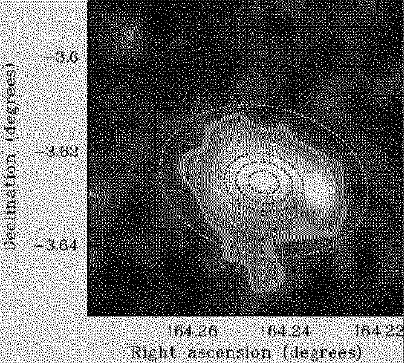
Figure 1.— The grey scale image shows the ROSAT/HRI data after applying a Gauss filter of $\sigma=8\arcsec$. The contours show the best fit elliptical cluster $\beta$–model ($\beta=0.73$, see also Tab.1). The spacing of the contours is linear. The lowest contour is at $9.47~{}10^{-4}{\rm/s/arcmin^{2}}$ with similar spacing between two contours.

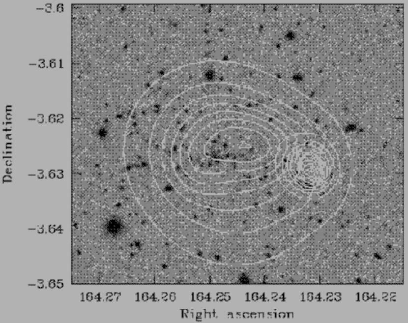
Figure 2.— Restored X-ray image from the wavelet analysis of the HRI raw image. The iso-intensity contours of the reconstructed main cluster and of the compact sub-substructure (in the west) are overlayed on the optical image (D98). The isocontours are linearly spaced by $6.1~{}10^{-4}~{}{\rm ct/s/arcmin^{2}}$, the value of the lowest contour.

Surface brightness profile of MS1054. The crosses show the data with 1$\sigma$ error bars. The full line is the best fit 1–D $\beta$–model . The dotted curves are the profiles of the best fit 2–D elliptical model $\pm 2\sigma$ errors on the central surface brightness ($\beta=0.73$).

Total and gas mass profiles of MS1054. The error bars correspond to the error on the imaging data. Full lines and dashed lines are the results of the 1–D and 2–D isothermal $\beta$–model fit respectively. Dashed-dotted lines: virial mass from numerical simulations at this redshift (Evrard et al. 1996). The heavy lines are for k$T=12.3{\rm\ keV}$. The thin lines correspond to the lower (k$T=10.1{\rm\ keV}$) and upper limit (k$T=15.4{\rm\ keV}$) of the ASCA temperature measurement.

Variation of the estimated gas mass fraction $f_{\rm gas}$ of MS1054-03 with the assumed cosmology. $f_{\rm gas}$ is normalized to the value obtained for $\Omega_{0}=1$. Full line: variation with $\Omega_{0}$ for an open Universe ($\Lambda=0$). Dotted line: flat $\Lambda$ dominated Universe. The X–ray parameters are fixed to their best fit values (${\rm k}T=12.3~{}{{\rm\ keV}},\beta=0.96,\theta_{\rm c}=0.89\arcmin$).

References

- (1) Arnaud, M.,& Evrard A. E. 1999, MNRAS, 305, 631
- (2) Arnaud, M., Maurogordato, S., Slezak, E., Rho, J., 2000, A&A, 355, 461
- (3) David, L. P., et al. 1997, The ROSAT High-Resolution Imager (HRI) calibration report (Washington: US ROSAT Science Data Center/ SAO)
- (4) Donahue, M., Voit, G. M., Gioia, I., Luppino, G., Hughes, J. P., & Stocke J.T. 1998, ApJ, 502, 550 (D98)
- (5) Ebeling, H. et al. 1999 astro-ph/9905321
- (6) Elbaz, D., Arnaud M., Böringer H., 1995, å, 293, 337
- (7) Evrard, A. E., Metzler, C. A.,& Navarro, J. F. 1996, ApJ, 469, 494
- (8) Gioia, I. M., Maccacaro, T., Schild, R. E., Wolter, A., & Stocke, J. T. 1990, ApJS, 72, 567
- (9) Jones, C.,& Forman, W. 1999, ApJ, 511, 65
- (10) Luppino, G. A.,& Kaiser N. 1997, ApJ, 475, 20
- (11) Neumann, D. M.,& Böhringer, H. 1997, MNRAS, 289, 123
- (12) Neumann, D. M. 1999, ApJ, 520, 87
- (13) Oukbir, J.,& Blanchard, A. 1992, A&A, 262, L21
- (14) Rué, F.,& Bijaoui, A., 1997, Experimental Astronomy 7, 129
- (15) Pen, U., 1997, New Astronomy, 2, 309
- (16) Press, W. H., Flannery, B. P., Teukolsky S. A.,& Vetterling W. T., 1986, Numerical Recipes, Cambridge University Press
- (17) Schindler, S. 1996, A&A, 305, 756
- (18) Schindler, S. 1999, A&A, 349, 435
- (19) Snodwen, S. L. 1998, ApJS, 117, 233
- (20) Voit, G. & Donahue, M., 1998, ApJ, 500, L111
- (21) Tran, K.-V., Kelson, D. D., Van Dokkum, P., Franx, M., Illingworth, G. D.,& Magee, D. 1999, ApJ, 522, 39
- (22) Trümper J. 1992, QJRAS, 33, 165