The Clustering of Colour Selected Galaxies

Abstract

We present measurements of the angular correlation function of galaxies selected from a $B_{J}\sim 23.5$ multicolour survey of two $5^{\circ}\times 5^{\circ}$ fields located at high galactic latitudes. The galaxy catalogue of $\sim 4\times 10^{5}$ galaxies is comparable in size to catalogues used to determine the galaxy correlation function at low-redshift. Measurements of the $z\sim 0.4$ correlation function at large angular scales show no evidence for a break from a power law though our results are not inconsistent with a break at $\ga 15h^{-1}{\mathrm{M}pc}$. Despite the large fields-of-view, there are large discrepancies between the measurements of the correlation function in each field, possibly due to dwarf galaxies within $z\sim 0.11$ clusters near the South Galactic Pole.

Colour selection is used to study the clustering of galaxies $z\sim 0$ to $z\sim 0.4$. The galaxy correlation function is found to strongly depend on colour with red galaxies more strongly clustered than blue galaxies by a factor of $\ga 5$ at small scales. The slope of the correlation function is also found to vary with colour with $\gamma\sim 1.8$ for red galaxies while $\gamma\sim 1.5$ for blue galaxies. The clustering of red galaxies is consistently strong over the entire magnitude range studied though there are large variations between the two fields. The clustering of blue galaxies is extremely weak over the observed magnitude range with clustering consistent with $r_{0}\sim 2h^{-1}{\mathrm{M}pc}$. This is weaker than the clustering of late-type galaxies in the local Universe and suggests galaxy clustering is more strongly correlated with colour than morphology. This may also be the first detection of a substantial low redshift galaxy population with clustering properties similar to faint blue galaxies.

1 Introduction

The galaxy two-point correlation function is commonly used to measure the structure of the galaxy environment from high redshift until the present epoch. The clustering properties of galaxies in the local Universe are well measured by large representative surveys of the galaxy population (Maddox, Efstathiou & Sutherland 1996). Catalogues of galaxies selected by morphology show large variations of the galaxy correlation function with late type galaxies having considerably weaker clustering than early type galaxies (Davis & Geller 1976, Loveday et al. 1995).

The results from studies of galaxies with fainter apparent magnitudes and higher redshifts are less conclusive. Pencil-beam surveys with CCDs and photographic plates from $4{\mathrm{m}}$ telescopes have measured the amplitude of the $B>22$ correlation function; however, estimates vary by $\ga 100\%$ (Infante & Pritchet 1995). Also, while $B>22$ surveys show evidence for a rapid decline of the amplitude of the correlation function (Efstathiou et al. 1991, Infante & Pritchet 1995, Roche et al. 1996), $I$ band imaging surveys to similar depths show no evidence for a rapid decrease of the correlation function amplitude (Postman et al. 1998).

The small areas of previous studies of the faint galaxy correlation function are a possible source of the discrepancy. Large individual structures and voids in the Universe could bias estimates of the correlation function if the field-of-view of the survey is small. The use of single band data to select catalogues of galaxies could suffer from biases as the morphological mix of galaxies will change as a function of limiting magnitude. It is probable that the differing amplitudes of the $B$ and $I$ band correlation functions are due to faint $B$ band data being dominated by weakly clustered blue galaxies (Efstathiou et al. 1991) while the $I$ band data has a larger fraction of early type galaxies.

In this paper, we use a $B_{J}\sim 23.5$ multicolour catalogue of galaxies derived from two $5^{\circ}\times 5^{\circ}$ fields to measure the clustering properties of faint galaxies. Section 2 discusses the observations and data reduction used to produce the galaxy catalogue. The method used to determine the angular and spatial correlation functions is described in Sections 3 and 4. Estimates of the correlation function at large angular scales are presented in Section 5. Section 6 discusses the angular correlation function as a function of limiting magnitude for the $U$, $B_{J}$, $R_{F}$ and $I$ bands. We show that it is impossible to use a single model to describe the observed clustering of galaxies as different populations of galaxies are measured by each band as a function of limiting magnitude. In Section 7, we use colour selection to measure galaxies with similar stellar populations over a range of redshifts. Our estimates of the spatial correlation function indicate clustering is more strongly correlated with colour than morphology. Our main conclusions are summarised in Section 8.

2 The Galaxy Catalogue

The image data consists of $U$, $B_{J}$, $R_{F}$ and $I$ band digitally coadded SuperCOSMOS scans of photographic plates of the South Galactic Pole Field (SGP) and UK Schmidt field 855 (F855). The field centres, number of photographic plates and limiting magnitudes for each field and band are listed in Table 1. The individual photographic plates were obtained with the $1.25{\mathrm{m}}$ UK Schmidt Telescope between 1977 and 1998 for various programmes. The field-of-view is $6.4^{\circ}\times 6.4^{\circ}$ though vignetting is greater than $0.1$ magnitudes at angular scales more than $\sim 3.35^{\circ}$ from the optical axis (Tritton 1983).

The individual plates were digitised with the SuperCOSMOS facility at Royal Observatory Edinburgh (Miller et al. 1991). The $10\mu{\mathrm{m}}$ pixels and $15\mu{\mathrm{m}}$ resolution of SuperCOSMOS corresponds to a pixel scale of $0.67^{\prime\prime}$ and allows good sampling of images obtained in typical seeing ($\sim 2.5^{\prime\prime}$). The plate scans were converted from transmission to approximate intensity space before stacking. All plates were sky-limited so faint objects are in the linear regime of the plate response.

Before coadding the individual plate scans, the background was subtracted with a $160\times 160$ pixel median filter. Without background subtraction, robust bad pixel rejection is not possible resulting in contamination of the catalogue. To reduce the computation time required to subtract the background, the background was calculated for $32\times 32$ pixel regions rather than for each pixel and only every 4th pixel in the $160\times 160$ filter box was used to determine the median. Before coadding the scans, the noise distribution of the individual plates was measured and found to be fitted accurately by a Gaussian curve. If the noise distribution was significantly skewed, large systematic errors would propagate into the coadded plate scans.

As faint objects are in the linear regime of the plate response and the noise distribution is approximately Gaussian, the IRAF task imcombine can be effectively used to coadd the data. An average of the plates weighted by the background noise and min-max bad pixel rejection is used to provide high signal-to-noise and robust bad pixel rejection. Without robust bad pixel rejection, there is significant contamination of the catalogue by plate-flaws, satellite trails and asteroids. For bands with 5 or less plates, the number of pixels rejected by the bad pixel rejection algorithm results in the coaddition effectively being a median. For the SGP $U$ band data, where only 2 of the 3 plates are of high quality, a weighted average with no bad pixel rejection is used and objects are correlated with the $B_{J}$, $R_{F}$ and $I$ catalogues to remove contamination. The $U$ band data is complete to $U=22$ for objects with $B_{J}$ detections but incompleteness does effect the catalogue at $U>21.5$ for faint galaxies with $U-B_{J}<-1.5$.

Object detection, instrumental photometry and faint object star-galaxy classifications are determined using SExtractor (Bertin & Arnouts 1996). In the non-linear regime of the plate response where SExtractor classifications are unreliable, objects are classified as stellar if they are within the stellar locus in peak intensity versus magnitude space and area versus magnitude space. The reliability of the object classifications is improved by using object classifications in multiple bands where possible. Objects with SExtractor classification scores greater than 0.7 in 3 bands, 0.75 in 2 bands or 0.85 in a single band are classified as stellar objects. Comparison of the object classification with the $B_{J}<22$ and $B<24$ spectroscopic samples of Colless et al. (1990) and Glazebrook et al. (1995) show the star-galaxy separation to be correct for $\sim 85\%$ of $B_{J}<23$ objects and contamination of the galaxy catalogue is $\la 5\%$. At $B_{J}<20$, comparison of object classifications with CCD images, eye-ball classifications and colour-colour diagrams indicates the reliability of the star-galaxy separation is $\ga 95\%$.

Photometric calibration of the data was obtained with $B$, $V$, $R$ and $I$ band CCD data from the Siding Spring 40-inch provided by Bruce Peterson, $B$ and $R$ band CCD imaging with the Anglo-Australian Telescope provided by Bryn Jones and $U$ band photometry from Croom et al. (1999) and Osmer et al. (1998). Galaxy and faint stellar photometry is obtained by adding a zero-point value to the instrumental magnitudes while bright stellar photometry is determined by a polynomial fit between the instrumental magnitudes and calibrated CCD magnitudes. All magnitudes are corrected for vignetting using a fit to the vignetting as a function of radius plot from Tritton (1983). Comparison of the photometry with Boyle, Shanks & Croom (1995), Caldwell & Schechter (1996), Croom et al. (1999), Osmer et al. (1998) and Patch B of the ESO Imaging Survey (Prandoni et al. 1999) limits zero point errors to less than $0.05$ magnitudes. Comparison of median colours as a function of limiting magnitude and galaxy loci in colour-colour diagrams show no significant offsets between the two fields.

Magnitude estimates for galaxies are corrected for dust extinction using the dust maps of Schlegel, Finkbeiner & Davis (1998). Figure 1 shows that there are significant variations in the dust extinction in F855 which could introduce spurious large-scale structure into the catalogue. In contrast, the dust extinction in the SGP is restricted to the range $0.01<E(B-V)<0.03$ which is a comparable to the $0.028$ magnitude error estimate of the dust maps. We therefore use the dust map estimates of the extinction for F855 while using a constant value of $E(B-V)=0.015$ to correct for dust extinction in the SGP.

Completeness limits for the catalogue are determined with comparison to deeper CCD images (where available) and number counts as a function of limiting magnitude (Figure 2). The number counts for the two fields are in good agreement with each other in all 4 bands. However, at $B_{J}<19$ and $B_{J}>21$ the number counts are slightly higher than those measured by Maddox et al. (1990) and Infante & Pritchet (1992). The resulting completeness limits for the four bands are $U=21.5$, $B_{J}=23.5$, $R_{F}=22$ and $I=20$ for the SGP and $U=22$, $B_{J}=23.5$, $R_{F}=22.5$ and $I=20$ for F855. Overestimates of the completeness limits would result in biases in estimates of the correlation function as vignetting would introduce spurious structure into the catalogue.

Table 1: Image data parameters

Field	RA (1950) DEC	Band	Limiting	# of
			Mag	Plates
SGP	$00^{\mathrm{h}}~{}53^{\mathrm{m}}$ $-28^{\circ}~{}03^{\prime}$	$U$	21.5	3
SGP	$00^{\mathrm{h}}~{}53^{\mathrm{m}}$ $-28^{\circ}~{}03^{\prime}$	$B_{J}$	23.5	9
SGP	$00^{\mathrm{h}}~{}53^{\mathrm{m}}$ $-28^{\circ}~{}03^{\prime}$	$R_{F}$	22	8
SGP	$00^{\mathrm{h}}~{}53^{\mathrm{m}}$ $-28^{\circ}~{}03^{\prime}$	$I$	20	5
F855	$10^{\mathrm{h}}~{}40^{\mathrm{m}}$ $00^{\circ}~{}00^{\prime}$	$U$	22	5
F855	$10^{\mathrm{h}}~{}40^{\mathrm{m}}$ $00^{\circ}~{}00^{\prime}$	$B_{J}$	23.5	12
F855	$10^{\mathrm{h}}~{}40^{\mathrm{m}}$ $00^{\circ}~{}00^{\prime}$	$R_{F}$	22.5	26
F855	$10^{\mathrm{h}}~{}40^{\mathrm{m}}$ $00^{\circ}~{}00^{\prime}$	$I$	20	7

Figure 1: A plot of the dust extinction across the SGP and F855 fields using $E(B-V)$ estimates from Schlegel, Finkbeiner & Davis (1998). The dust extinction in F855 ($l\sim 45^{\circ}$) is significantly larger and shows more structure than the SGP. The extinction in F855, if left uncorrected, would introduce spurious structure on large angular scales.

Figure 2: A plot of the galaxy number counts as a function of magnitude (after correction for dust extinction). Data from both fields is compared with number counts from the APM survey (Maddox et al. 1990) and Infante & Pritchet (1992). $I$ band counts have been moved 1 magnitude to the left and $U$ band counts have been moved 2 magnitudes to the right for clarity.

Contamination of the catalogue by spurious objects biases estimates of the galaxy correlation function and these have to be removed. Most plate-flaws, asteroids and satellite trails are effectively removed by the bad-pixel rejection algorithm. The plate edges, the step wedges, globular clusters, bright galaxies and the internal reflections of $V<5$ stars are manually removed from the catalogue. The majority of the remaining contaminating objects are diffraction spikes and halos around bright stars and these are removed with a program that drills regions around bright stars. Spurious structure may also be introduced into the catalogue at angular scales more than $3.35^{\circ}$ from the plate centre where number counts are altered by $>10\%$ during the vignetting correction. To prevent this, the corners of the fields have been excluded from the catalogue. The resulting geometry of the $5^{\circ}\times 5^{\circ}$ field-of-view is shown in Figure 3. The final catalogues of galaxies contain $\sim 2\times 10^{5}$ galaxies per field in both $B_{J}$ and $R_{F}$.

Figure 3: A flux weighted map of $R_{F}<22$ galaxies in the SGP. The dark blocks are regions which have been removed from the catalogue. The corners of both fields have been removed to prevent objects with significant vignetting entering the catalogue. Some of the Abell clusters in the field can be seen as overdense regions.

3 Estimation of the Angular Correlation Function

The galaxy two-point correlation function, $\omega(\theta)$, measures the mean excess surface density of pairs at angular separation $\theta$ compared with the expected number of pairs if galaxies were randomly distributed. The most commonly used estimator of the angular correlation function is

$$\hat{\omega}(\theta)=\frac{DD}{DR}-1$$ (1)

where $DD$ and $DR$ are the number of galaxy-galaxy and galaxy-random object pairs at angular separations $\theta\pm\delta\theta$. The random objects are typically copies of real objects distributed randomly across the field-of-view. To reduce errors, multiple random copies of each object can be made and the estimate of $DR$ renormalised. However, the $DD/DR$ estimator is subject to first-order errors in the galaxy density contrast (Hamilton 1993) making it unsuitable for measuring weak clustering at large angular scales. We therefore use an estimator with lower variance than $DD/DR$, the estimator

$$\hat{\omega}(\theta)=\frac{DD-2DR+RR}{RR}$$ (2)

(Landy & Szalay 1993) where $RR$ is the number of random-random object pairs at angular separations $\theta\pm\delta\theta$. The value of $\hat{\omega}(\theta)$ is determined for different angular scale bins with the values of $DD$, $DR$ and $RR$ being determined with pairs of individual objects at small angular scales and weighted pairs of cells containing multiple objects at large angular scales. The use of cells to determine the angular correlation function reduces the computational time required to several hours and does not introduce significant errors.

The estimator of the angular correlation function satisfies the integral constraint,

$$\int\int\hat{\omega}(\theta)\delta\Omega_{1}\delta\Omega_{2}\simeq 0$$ (3)

(Groth and Peebles 1977), resulting in an underestimate of the angular correlation function. To remove this bias from the correlation function, the term

$$\omega(\theta)_{\Omega}=\frac{1}{\Omega^{2}}\int\int\omega(\theta)\delta\Omega_{1}\delta\Omega_{2}$$ (4)

is added to the estimate of the correlation function. The term, $\omega(\theta)_{\Omega}$ does require an assumption of the form of the correlation function to correctly estimate the value of correlation function. However, previous work with smaller fields of view and at brighter limiting magnitudes shows that the angular correlation is well approximated by a power law at angular scales less than $1^{\circ}$ (Maddox, Efstathiou & Sutherland 1996).

A further source of bias in estimates of the correlation function is contamination of the catalogue by randomly distributed objects such as stars. If the fraction of the catalogue contaminated by stars is $f$, the estimate of the correlation function is reduced by a factor of $(1-f)^{2}$ at all angular separations. As mentioned previously, comparison with spectroscopic samples indicates the star galaxy separations if $\ga 85\%$ reliable at magnitude brighter than $B_{J}<22$. At fainter magnitudes, the contamination of the catalogue by stars is negligible as galaxies consist more than $\ga 80\%$ of the object number counts at $B_{J}\geq 23$ (Glazebrook et al. 1995).

4 Modelling the Spatial Correlation Function

For this work, we assume that the spatial correlation function is a power law of the form,

$$\xi(r,z)=\left(\frac{r}{r_{0}}\right)^{-\gamma}(1+z)^{-(3+\epsilon)},$$ (5)

(Efstathiou et al. 1991) where $r$ is the spatial separation in physical coordinates, $z$ is the redshift and $r_{0}$, $\gamma$ and $\epsilon$ are constants. If $\epsilon=0$ the clustering is fixed in physical coordinates while if $\epsilon=\gamma-3$ the clustering is fixed in comoving coordinates. This parameterisation of the evolution of the spatial correlation function is not valid at all redshifts but is a good approximation at $z<1$ (Baugh et al. 1999). For galaxies selected with images in a single broadband, typical values of the parameters of $\xi(r,z)$ are $r_{0}\sim 5h^{-1}{\mathrm{Mpc}}$, $\gamma\sim 1.7$ (Maddox, Efstathiou & Sutherland 1996) and $\epsilon\sim-1$.

For a power law spatial correlation function, the resulting angular correlation function is a power law with

$$\omega(\theta)=\sqrt{\pi}\frac{\Gamma[(\gamma-1)/2]}{\Gamma(\gamma/2)}Br_{0}^{\gamma}\theta^{(1-\gamma)}$$ (6)

(Baugh & Efstathiou 1993) where $B$ is a constant. The value of $B$ is given by

$$B=\int^{\infty}_{0}g(z)\left(\frac{dN(z)}{dz}\right)^{2}dz\left/\left[\int^{\infty}_{0}\frac{dN(z)}{dz}dz\right]^{2}\right.$$ (7)

where

$$g(z)=\frac{dz}{dx}x^{1-\gamma}F(x)(1+z)^{-(3+\epsilon-\gamma)},$$ (8)

$x$ is the coordinate distance at redshift z, $dN/dz$ is the number of galaxies per unit redshift detected by the survey and

$$F(x)^{2}=1+\Omega_{R}(H_{0}x/c)^{2}.$$ (9)

The value of $x$ is given by

$$x=\frac{c}{H_{0}}\int^{z}_{0}\frac{1}{E(z)}$$ (10)

where

$$E(z)\equiv\sqrt{\Omega_{M}(1+z)^{3}+\Omega_{R}(1+z)^{2}+\Omega_{\Lambda}}.$$ (11)

For values of $z<0.5$, the value of $B$ is more strongly dependent on $r_{0}$, $\gamma$ and the galaxy redshift distribution than the cosmological model. This is not unexpected as the value of $x$ for $z=0.4$ varies by less than $10\%$ between $\Omega_{M}=1$ and $\Omega_{M}=0.2$ models of the Universe. We therefore only use a single cosmological model with $H_{0}=75{\mathrm{k}ms}^{-1}{\mathrm{M}pc}^{-1}$, $\Omega_{M}=0.2$ and $\Omega_{\Lambda}=0$.

There are two approaches to modelling the galaxy redshift distribution which are often used in the literature. The first approach uses an accurate description of the local luminosity function of different galaxy types, plus models of galaxy evolution and k-corrections for each type, and attempts to model the observed number counts and redshift distribution where data is available (i.e. Roche et al. 1996). This model includes the physics of galaxy evolution, however, it contains large numbers of free parameters and different models can readily reproduce the observed number counts. The second approach, which is applied to our single band imaging data, assumes a functional form for the redshift distribution and uses the observed number counts and redshift surveys to constrain the model (Baugh & Efstathiou 1993). This approach produces a good model of the redshift distribution but contains no physics of galaxy evolution and is limited by the depth of redshift surveys.

To model the redshift distribution, we use the model of Baugh & Efstathiou (1993). For a complete sample of galaxies brighter than magnitude $m$, the number of galaxies detected per unit redshift is given by

$$\frac{dN(z)}{dz}=A(m)z^{2}{\rm exp}\left(-\left[\frac{z}{1.412z_{m}(m)}\right]^{3/2}\right)$$ (12)

where

$$A(m)=\frac{1.062N(m)\Omega}{z_{m}(m)},$$ (13)

$N(m)$ is the galaxy number counts, $\Omega$ is the survey area and $z_{m}$ is the median redshift of the galaxy sample. As the value of $B$ depends on the galaxy redshift distribution and not the galaxy number counts, the most important free parameter is $z_{m}$ which is a function of band and limiting magnitude.

The median redshift as a function of limiting magnitude is obtained from a polynomial fit to median redshifts derived from galaxy redshift surveys. At low redshift this is derived from the local galaxy luminosity function while at higher redshifts the median redshifts determined directly from the survey data are used. Local luminosity functions are assumed to be Schechter functions with $\alpha=-1.00$,

$$M^{*}_{B_{J}}=-19.5-5{\mathrm{l}og}h$$ (14)

Loveday et al. (1992) and

$$M^{*}_{R_{F}}=-20.5-5{\mathrm{l}og}h.$$ (15)

Changing the value of $\alpha$ to $-1.3$ reduces the estimate of the median redshift by $\sim 15\%$ resulting in a similar decrease of the estimate of $r_{0}$. Galaxy $k$-corrections are approximated by $k_{B}(z)=2z$ and $k_{R}(z)=0.5z$. At $z\ga 0.2$, median redshifts as a function of survey depth are derived from the redshift surveys of Colless et al. (1990), Glazebrook et al. (1995), Lin et al. (1999) and Munn et al. (1997). $I$ band median redshifts are the same as Postman et al. (1998) which were derived from the CFHT redshift survey (Lilly et al. 1995). To determine the $U$ band median redshift, we use $U-B_{J}\sim 0.3$, the median colour of $B_{J}<21$ galaxies in the F855 field. The functions for median redshift as a function of limiting magnitude are shown in Figure 4.

Figure 4: A plot of the model median redshift as a function of survey depth for $U$, $B_{J}$, $R_{F}$ and $I$ bands. The median redshift for the $U$ band is derived using a median galaxy colour of $U-B_{J}\sim 0.3$. Magnitude limits for the SGP and F855 are shown with the large filled and open circles respectively.

5 The Angular Correlation Function at Large Angular Scales

The $5^{\circ}\times 5^{\circ}$ field-of-view of each field allows the measurement of the faint galaxy correlation function at large angular scales. At $B_{J}\sim 23.5$ and $R_{F}\sim 22$, the median redshift of the data is $z\sim 0.4$ and a break in the spatial correlation function at $\sim 15h^{-1}{\mathrm{Mpc}}$ in comoving coordinates (Maddox, Efstathiou & Sutherland 1996) corresponds to an angular scale of $\sim 1^{\circ}$.

It is possible to measure the angular correlation for each field to $\sim 5^{\circ}$ but at large angular scales the estimate of the correlation function will be dominated by individual structures. To determine the range of angular scales where the correlation function is representative, we compare the estimates of the angular correlation function for the SGP and F855 fields. This provides a more reliable estimate than subsamples of the data as each subsample would have smaller field-of-view than the original data, resulting in overestimates of the errors at large angular scales.

The $B_{J}<23.5$ and $R_{F}<22$ correlation functions for each field are shown in Figures 5 and 6. As the integral constraint depends of $\gamma$, the data has been fitted with power laws with fixed $\gamma$ to allow comparison of the 2 fields estimates of $\omega(\theta)$. For both fields the integral constraint is less than the amplitude of the correlation function at $1^{\circ}$. A power law matches the data well and there is no evidence of a break from a power law on all angular scales. However, on angular scales $\ga 2^{\circ}$, the estimates of $\omega(\theta)$ for both fields are within $2\sigma$ of $0$. It is therefore possible that the break in the correlation function is present at $15h^{-1}{\mathrm{M}pc}$ in comoving coordinates but can not be detected with this dataset.

Figure 5: The $B_{J}<23.5$ angular correlation function for the SGP and F855 fields. Power law fits to the SGP and F855 data are shown with solid and dashed lines respectively. The data in each field is fitted well by a power law and most data points are within $2\sigma$ of each other. There is no evidence of a break in the correlation function on any of the scales measured though $\omega(\theta)$ at $>1^{\circ}$ is only $\sim 2\sigma$ more than 0. It is also possible both correlation functions could be biased by large structures on scales $>1^{\circ}$.

Figure 6: The $R_{F}<22$ angular correlation function for the SGP and F855 fields. Power law fits to the SGP and F855 data are shown with solid and dashed lines respectively. The data for each field is fitted well by a power law and there is no evidence of a break in the correlation function on scales less than $\sim 2^{\circ}$. However, unlike the $B_{J}<23.5$ data, there is an offset between the data in the two fields.

6 The Correlation Function as a Function of Limiting Magnitude

The large fields-of-view used for this study reduce the errors associated with large structures along the line-of-sight. Also, the input catalogue of up to $2.5\times 10^{5}$ galaxies results in small random errors in estimates of $\omega(\theta)$. Previous measures of the correlation function in $U$, $B_{J}$ and $R_{F}$ have been restricted to fields-of-view less than $\sim 2^{\circ}\times 2^{\circ}$ (Infante & Pritchet 1995). At the present time, only the $I$ band survey by Postman et al. (1998) has a comparable field-of-view with greater depth than this work.

Previous measurements of $\gamma$ indicate that it may vary with band and survey depth (Infante & Pritchet 1995, Postman et al. 1998) though most values in the literature are between $1.6$ and $1.8$. The consistent data reduction method used for this work should allow the accurate comparison of $\gamma$ as a function of band and survey depth.

Estimates of the value of $\omega(1^{\prime})$ and $\gamma$ derived from power law fits to the data are shown in Table 2. The amplitude of the correlation function is determined at $1^{\prime}$ rather than $1^{\circ}$ as the amplitude and $\gamma$ are not independent and estimates of $\omega(1^{\circ})$ depend strongly on $\gamma$. The values of $\gamma$ show a weak trend towards smaller values with magnitude and bluer survey bands. As there is a correlation between galaxy colour and morphology (see Figure 11) and late type galaxies have shallower values of $\gamma$ than early type galaxies, this trend is not unexpected.

Table 2: Measured parameters for $\omega(\theta)$ determined from power law fits to data between $10^{\prime\prime}$ and $0.3^{\circ}$.

Field	SGP			F855
Magnitude Range	$N_{gal}$	$\gamma$	$\omega(1^{\prime})\times 10^{3}$	$N_{gal}$	$\gamma$	$\omega(1^{\prime})\times 10^{3}$
$18.0\leq U\leq 20.0$	4309	$1.39\pm 0.18$	$418\pm 151$	4913	$1.53\pm 0.27$	$239\pm 52$
$18.0\leq U\leq 21.0$	16379	$1.65\pm 0.10$	$196\pm 16$	16695	$1.84\pm 0.10$	$125\pm 16$
$18.0\leq U\leq 22.0$	80502	$1.47\pm 0.10$	$63\pm 4$	82965	$1.47\pm 0.15$	$37\pm 5$
$18.0\leq B_{J}\leq 20.0$	5267	$1.58\pm 0.15$	$530\pm 85$	5486	$1.76\pm 0.17$	$335\pm 62$
$18.0\leq B_{J}\leq 21.0$	15372	$1.60\pm 0.12$	$280\pm 32$	15149	$1.72\pm 0.12$	$196\pm 27$
$18.0\leq B_{J}\leq 22.0$	45519	$1.53\pm 0.07$	$122\pm 7$	43743	$1.66\pm 0.11$	$90\pm 8$
$18.0\leq B_{J}\leq 22.5$	82919	$1.48\pm 0.09$	$72\pm 5$	76149	$1.60\pm 0.07$	$56\pm 4$
$18.0\leq B_{J}\leq 23.0$	144577	$1.53\pm 0.07$	$45\pm 2$	123325	$1.47\pm 0.08$	$38\pm 2$
$18.0\leq B_{J}\leq 23.5$	230024	$1.46\pm 0.07$	$28\pm 1$	184717	$1.49\pm 0.05$	$31\pm 2$
$16.5\leq R_{F}\leq 18.5$	4330	$1.68\pm 0.10$	$586\pm 80$	4294	$1.82\pm 0.17$	$397\pm 82$
$16.5\leq R_{F}\leq 19.5$	13752	$1.72\pm 0.07$	$346\pm 50$	12841	$1.81\pm 0.13$	$232\pm 32$
$16.5\leq R_{F}\leq 20.5$	39748	$1.70\pm 0.03$	$179\pm 9$	37069	$1.80\pm 0.08$	$130\pm 12$
$16.5\leq R_{F}\leq 21.5$	112919	$1.58\pm 0.05$	$72\pm 3$	102373	$1.70\pm 0.07$	$61\pm 4$
$16.5\leq R_{F}\leq 22.0$	174385	$1.57\pm 0.05$	$54\pm 2$	173295	$1.60\pm 0.05$	$43\pm 2$
$16.5\leq R_{F}\leq 22.5$	-	-	-	234957	$1.65\pm 0.07$	$32\pm 2$
$16.5\leq I\leq 18.5$	9812	$1.73\pm 0.07$	$322\pm 26$	8913	$1.82\pm 0.15$	$254\pm 41$
$16.5\leq I\leq 19.5$	32178	$1.67\pm 0.06$	$156\pm 11$	28365	$1.79\pm 0.12$	$115\pm 14$
$16.5\leq I\leq 20.0$	54737	$1.71\pm 0.05$	$108\pm 8$	48743	$1.80\pm 0.08$	$93\pm 8$

While the value of $\gamma$ does not differ by more then $\sim 2\sigma$ between the two fields, the amplitude of the correlation function varies by $\sim 100\%$ at bright magnitudes. While variations of amplitude could be caused by zero point errors, the error required is approximately $0.4$ magnitudes in all bands at bright magnitudes with it decreasing to $\sim 0$ at $B_{J}\sim 23$. This is inconsistent with the photometric calibration, the galaxy number counts in Figure 2 and the colour-colour diagrams. A systematic error could be present in the data but it seems unlikely that it could effect $\omega(1^{\prime})$ without causing large variations of $\gamma$.

If the values of $\omega(1^{\prime})$ do not have significant systematic errors, a possible cause of the variations is that the two fields measure different populations of galaxies with different clustering properties. The SGP, which has stronger clustering than F855, contains “sheets” perpendicular to the line-of-sight (Broadhurst et al. 1990) and smaller structures including 22 Abell clusters (Abell, Corwin & Olowin 1989). Of these clusters, 11 appear to be associated with a structure at $z\sim 0.11$ identified by Broadhurst et al. (1990). $M_{B_{J}}\sim-19.5$ ($M^{*}$) galaxies at $z\sim 0.11$ have an apparent magnitude of $B_{J}\sim 18$ and this population of galaxies is too small to significantly bias estimates of the $B_{J}>20$ correlation function. However, it is possible that the cluster population of $M_{B_{J}}\ga-16$ galaxies could bias estimates of the correlation function if they are a significant fraction of the observed galaxy number counts.

To test if the $z=0.11$ clusters do significantly effect the correlation function, the correlation function has been determined with $2^{\circ}\times 2^{\circ}$ ($\sim 10h^{-1}{\mathrm{M}pc}\times 10h^{-1}{\mathrm{M}pc}$) regions surrounding the clusters removed from the data. As the clusters are not uniformly distributed across the field-of-view, the size of the catalogue is reduced by $\sim 60\%$. Table 3 lists the amplitude of the $B_{J}$ and $R_{F}$ band correlation functions for the SGP field without the clusters and F855 for comparison. The amplitude of the correlation function has decreased significantly compared with the original estimates for the SGP. While most noticeable at bright magnitudes, the effect is also significant at fainter magnitudes where the contribution from nearby clusters might be expected to be small. This is consistent with $M_{B_{J}}\ga-16$ galaxies within the clusters significantly effecting estimates of the faint galaxy correlation function. However, details of the relationship between clusters and the observed clustering of faint galaxies will be explored in a later paper.

Table 3: Measured parameters for $\omega(\theta)$ determined from power law fits to data between $10^{\prime\prime}$ and $0.3^{\circ}$. Clusters at $z\sim 0.11$ have been removed from the SGP sample to reduce the effect dwarf galaxies may have on the estimate of the correlation function.

Field	SGP (no $z=0.11$ clusters)			F855
Magnitude Range	$N_{gal}$	$\gamma$	$\omega(1^{\prime})\times 10^{3}$	$N_{gal}$	$\gamma$	$\omega(1^{\prime})\times 10^{3}$
$18.0\leq B_{J}\leq 20.0$	1742	$1.95\pm 0.35$	$530\pm 85$	5486	$1.76\pm 0.17$	$335\pm 62$
$18.0\leq B_{J}\leq 21.0$	5487	$1.76\pm 0.20$	$200\pm 44$	15149	$1.72\pm 0.12$	$196\pm 27$
$18.0\leq B_{J}\leq 22.0$	16679	$1.72\pm 0.12$	$108\pm 11$	43743	$1.66\pm 0.11$	$90\pm 8$
$18.0\leq B_{J}\leq 22.5$	30886	$1.61\pm 0.17$	$60\pm 8$	76149	$1.60\pm 0.07$	$56\pm 4$
$18.0\leq B_{J}\leq 23.0$	54549	$1.54\pm 0.15$	$36\pm 4$	123325	$1.47\pm 0.08$	$38\pm 2$
$18.0\leq B_{J}\leq 23.5$	87453	$1.56\pm 0.16$	$22\pm 3$	184717	$1.49\pm 0.05$	$31\pm 2$
$16.5\leq R_{F}\leq 18.5$	1460	$2.16\pm 0.14$	$339\pm 170$	4294	$1.82\pm 0.17$	$397\pm 82$
$16.5\leq R_{F}\leq 19.5$	4974	$1.84\pm 0.18$	$223\pm 30$	12841	$1.81\pm 0.13$	$232\pm 32$
$16.5\leq R_{F}\leq 20.5$	14481	$1.76\pm 0.13$	$144\pm 12$	37069	$1.80\pm 0.08$	$130\pm 12$
$16.5\leq R_{F}\leq 21.5$	41767	$1.67\pm 0.11$	$65\pm 6$	102373	$1.70\pm 0.07$	$61\pm 4$
$16.5\leq R_{F}\leq 22.0$	65168	$1.71\pm 0.10$	$49\pm 2$	173295	$1.60\pm 0.05$	$43\pm 2$

For the following discussion of the amplitude as a function of limiting magnitude, the estimates of the SGP correlation function including the $z=0.11$ clusters are used. While it is probable relatively nearby clusters do effect estimates of the correlation function, there is no clear justification for excluding them. Also, excluding the regions surrounding the clusters significantly reduces the number of galaxy pairs used to determine the correlation function, significantly increasing random errors.

Figures 7 to 10 plot the $I$, $R_{F}$, $B_{J}$ and $U$ band angular correlation function amplitudes as a function of limiting magnitude. The amplitude of the correlation function has been determined with fixed values of $\gamma$ to reduce the dependence of the amplitude on $\gamma$. As the values of the angular correlation function differ significantly between each field, no attempt has been made to fit the data. Instead, a model has been plotted with clustering fixed in comoving coordinates and $r_{0}=5h^{-1}{\rm Mpc}$. The value of $r_{0}$ is similar to values derived by Maddox, Efstathiou & Sutherland (1996) and Postman et al. (1998).

Figure 7: The $I$ band correlation function amplitude. The measurements of the amplitude are consistent with the data of Postman et al. (1998) which is shown with crosses. The data from Postman et al. (1998) has been corrected for the assumption that $\gamma=1.7$.

Figure 8: The $R_{F}$ band correlation function amplitude. While the redshift range is similar to the $I$ band data, the galaxy clustering is significantly weaker.

Figure 9: The $B_{J}$ band correlation function amplitude. As with the $R_{F}$ band data, the amplitude of the correlation function is significantly weaker than the $I$ band correlation function. At magnitudes fainter than $B_{J}\sim 22$, the correlation function rapidly decreases with limiting magnitude. There is also a decrease in the discrepancy between the SGP and F855 measurements with increasing limiting magnitude.

Figure 10: The $U$ band correlation function amplitude. The amplitude of the correlation function is consistently weaker than the fit to the $I$ band data shown with the dashed line.

Figure 7 shows the measured amplitude of the $I$ band correlation function for the SGP, F855 and Postman et al. (1998). The measured clustering in the SGP is in good agreement with Postman et al. (1998), while F855 measures slightly weaker clustering. The model of the clustering is also a reasonable estimate of the observed clustering across the magnitude range observed. Figures 8 to 10 show the $R_{F}$, $B_{J}$ and $U$ band clustering to be significantly weaker than the $I$ band clustering for galaxies with a similar range of redshifts. Comparison with the results of Infante & Pritchet (1995) show the SGP has similar clustering in $B_{J}$ and weaker clustering in $R_{F}$. Infante & Pritchet (1995) may measure stronger clustering than F855 as their field is located in the NGP which has similar large scale structures as the SGP (Broadhurst et al. 1990).

While the $r_{0}=5.0h^{-1}{\mathrm{M}pc}$ model is a good fit to the SGP $R_{F}<20$ and $B_{J}<21$ data, at fainter magnitudes a rapid decline in the amplitude of the correlation function is observed. The rapid decline of the faint correlation function has been observed previously by Efstathiou et al. (1991), Infante & Pritchet (1995) and Roche et al. (1996). Obviously, the $R_{F}$ and $B_{J}$ band data are sampling a different population of galaxies to the $I$ band sample. To be consistent with galaxy redshift surveys, the $B_{J}\sim 23$ galaxies must be dominated by a population of weakly ($r_{0}\sim 2.0h^{-1}{\mathrm{M}pc}$) clustered galaxies at $z\sim 0.4$ (Efstathiou et al. 1991, Efstathiou 1995).

For a no-evolution model for the galaxy population, the blue bands will sample galaxies with bluer colours due to the large k-corrections of early-type galaxies (Coleman, Wu & Weedman 1980). As shown in Figure 11, the local population of blue ($U-B_{J}\la 0$) galaxies is dominated by late-type galaxies. Measurements of the galaxy clustering in the local universe with morphology-selected catalogues show the clustering of late-type galaxies is considerably weaker than early-type galaxies (Davis & Geller 1976, Loveday et al. 1995). If the colours and clustering of $z\sim 0.4$ late and early type galaxies are similar to $z\sim 0$ galaxies, the decrease in the amplitude of the $B_{J}$ angular correlation function could be a selection effect. While it is impossible to determine the morphologies of the $B_{J}>21$ galaxies with this catalogue, it should be possible to use colour selection to select early and late type galaxies over a range of redshifts.

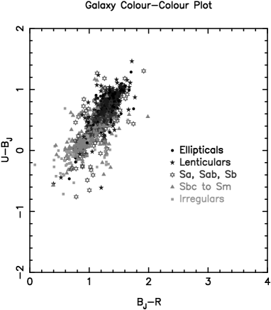
Figure 11: The colours of RC3 catalogue (de Vaucouleurs et al. 1991) galaxies by morphological type. Photometry is from Prugniel & Heraudeau (1998) while morphological classification of galaxies is from de Vaucouleurs et al. (1991). The correlation between morphology and colour can be clearly seen with late type galaxies generally having bluer colours than early types.

7 The Correlation Function of Colour Selected Galaxies

The obvious colour selection criteria for galaxies is a single colour cut in the deepest bands available ($B_{J}$ and $R_{F}$). However, as shown in Figure 12, the colour of individual galaxy types varies with redshift. Even with a single colour cut, the blue subsample will generally select later type galaxies than the red subsample and blue subsamples generally show weak clustering (Infante & Pritchet 1995, Roche et al. 1996). A $B_{J}-R_{F}$ cut that varies with magnitude may select the same population over a range of redshifts but the selection criteria would depend on the cosmological parameters used. Also, colour selection of a fraction of galaxies (i.e. the reddest $20\%$ of the catalogue) may not be effective due to the changing morphological mix of galaxies with magnitude.

Figure 12: The colour selection criteria for the red and blue subsamples. Colours of early, late and irregular type galaxies at $z=0$, $z=0.2$, $z=0.5$ and $z=0.8$ from Fukugita, Shimasaku & Ichikawa (1995) are shown. The colour selection criteria for each subsample are shown with the dot-dash line. The blue subsample consists of galaxies below and to the left of the line while the red subsample consists of galaxies above and to the right of the line. The blue subsample is dominated by late and irregular type galaxies while the red subsample selects early type galaxies.

Figure 13: Galaxy colour-colour diagrams for the SGP shown with the selection criteria for the two subsamples.

Selection of galaxies with two or more colour criteria should allow the selection of galaxy types over a large range of redshifts without strong dependence on cosmological parameters. Figure 12 shows the predicted colours of early, late and irregular type $0\leq z\leq 0.8$ galaxies from Fukugita, Shimasaku & Ichikawa (1995). Colour selection criteria for a red and blue subsample are also shown. The samples are limited to $B_{J}<21.6$ due to the $U=22$ magnitude limit of the catalogues and the $U-B_{J}>0.4$ selection criteria. As most $B_{J}<21.6$ galaxies are at redshifts $z\leq 0.3$, most galaxies in the subsamples are selected with the $U-B_{J}$ selection criteria. Galaxies with $U-B_{J}$ lower limits and $B_{J}-R_{F}$ upper limits have been included in the subsamples to prevent incompleteness. Figure 13 shows the colours of galaxies in the SGP with the subsample selection criteria. The location of the $B_{J}<19.5$ galaxy locus is similar to that for RC3 catalogue galaxies in Figure 11 though at $B_{J}>19.5$ there is an increasing fraction of very blue galaxies. Galaxy number counts for the 2 subsamples are shown in Figure 14. While the SGP does include significantly more clusters than F855 at low redshift, there is good agreement between the number counts across the magnitude range observed.

Figure 14: A plot of the red and blue subsample number counts for the SGP and F855.

While the selection criteria are relatively simple, it can be clearly seen that the red and blue subsample should select early and late type galaxies respectively. The blue subsample should also contain most of the galaxies with significant star formation rates while the red subsample should contain more passive galaxies. As shown in Figure 15, comparison with the spectroscopic catalogue of Colless et al. (1990) shows that most of the $[{\mathrm{O}II}]~{}3727{\mathrm{\AA}}$ emitters detected in the SGP and F855 are included in the blue subsample. To measure the clustering of starforming galaxies Cole et al. (1994) selected galaxies with $[{\mathrm{O}II}]~{}3727{\mathrm{\AA}}$ equivalent widths greater than $19{\mathrm{\AA}}$; all galaxies matching this selection criteria would be included in the blue subsample for both fields. Interestingly, the galaxies without $[{\mathrm{O}II}]~{}3727{\mathrm{\AA}}$ emission do not show such an obvious trend with similar numbers in both subsamples. However, the small number of galaxies without $[{\mathrm{O}II}]~{}3727{\mathrm{\AA}}$ emission results in these galaxies comprising less than $15\%$ of the total of blue galaxies.

Figure 15: A colour-colour diagram of $B_{J}<21.5$ galaxies in the SGP and F855 with spectroscopic observations by Colless et al. (1990). Lower limits in $U-B_{J}$ are shown with arrows. A trend towards bluer colours with $[{\mathrm{O}II}]~{}3727{\mathrm{\AA}}$ emission can be observed with strong $[{\mathrm{O}II}]~{}3727{\mathrm{\AA}}$ emitters restricted to the blue subsample.

The $B_{J}<21.5$ angular correlation functions of the blue and red subsamples of F855 are shown in Figure 16. Visual inspection shows the significant difference in clustering strength and the value of $\gamma$ for the two subsamples with the red subsample being strongly clustered and having a higher value of $\gamma$. This trend is consistent with measurements of the angular correlation functions of morphology selected catalogues where $\gamma\sim 1.8$ for early-type galaxies and $\gamma\sim 1.5$ for late-type galaxies (Loveday et al. 1995).

Figure 16: The $B_{J}<21.5$ angular correlation function for the red and blue subsamples of F855. The red subsample shows stronger clustering and a higher value of $\gamma$, consistent with the strong clustering of elliptical and early type galaxies in the local universe.

Table 4: Measured parameters for $\omega(\theta)$ for the red and blue subsamples determined from power law fits to data between $10^{\prime\prime}$ and $0.3^{\circ}$.

Field		SGP			F855
Sample	Magnitude Range	$N_{gal}$	$\gamma$	$\omega(1^{\prime})\times 10^{3}$	$N_{gal}$	$\gamma$	$\omega(1^{\prime})\times 10^{3}$
Blue	$18.0\leq B_{J}\leq 20.0$	2963	$1.45\pm 0.51$	$212\pm 3200$	3354	$1.41\pm 0.58$	$170\pm 2710$
Blue	$18.0\leq B_{J}\leq 21.0$	9079	$1.49\pm 0.18$	$138\pm 27$	9228	$1.61\pm 0.38$	$110\pm 39$
Blue	$18.0\leq B_{J}\leq 21.5$	15579	$1.57\pm 0.20$	$86\pm 19$	14329	$1.51\pm 0.32$	$75\pm 32$
Red	$18.0\leq B_{J}\leq 20.0$	1993	$1.65\pm 0.22$	$1339\pm 278$	1851	$2.09\pm 0.17$	$954\pm 210$
Red	$18.0\leq B_{J}\leq 21.0$	5552	$1.69\pm 0.12$	$782\pm 73$	5424	$1.89\pm 0.13$	$480\pm 82$
Red	$18.0\leq B_{J}\leq 21.5$	9317	$1.72\pm 0.08$	$616\pm 51$	9922	$1.83\pm 0.14$	$319\pm 44$

Estimates of $\gamma$ and $\omega(1^{\prime})$ as a function of limiting magnitude are listed in Table 4. The $z\sim 0.11$ clusters in the SGP have been retained in the data as there is no obvious justification for rejecting them from the sample. While $\gamma$ differs significantly between the two subsamples, the values of $\gamma$ are within $1\sigma$ of being constant as a function of limiting magnitude. The values of $\omega(1^{\prime})$ for the blue subsamples are remarkably similar for the SGP and F855. However, the red subsamples show large differences with the amplitude of the clustering in the SGP being $\sim 100\%$ larger than F855.

To model the spatial correlation function, a model of the redshift distribution for the red and blue subsamples is required. Luminosity functions for galaxies selected by morphology are available but it is not clear if luminosity is more or less strongly correlated with colour than morphology. We therefore use the $U-B_{J}<0.2$ and $U-B_{J}>0.2$ galaxy luminosity functions of Metcalfe et al. (1998). Approximate $k-$corrections of $k(z)=3z$ and $k(z)=z$ are used for the red and blue subsample respectively. We use the Metcalfe et al. (1998) luminosity functions rather than the redshift distribution model as the steep slope of faint end of the luminosity functions results in skewed redshift distributions.

Plots of the estimated median redshift for the red and blue luminosity functions are shown in Figures 17 and 18. The SGP and/or F855 overlap the $B_{J}$ magnitude limited redshift surveys of Colless et al. (1990) and Ratcliffe et al. (1998) which have been used to measure the median redshifts of the red and blue subsamples as a function of magnitude. In addition, $\sim 700$ galaxy redshifts are available from the NASA/IPAC Extragalactic Database (NED) and these have been used to show the approximate median redshift as a function of magnitude. For both subsamples, the model is a reasonable estimate of the redshift with few data points being more than $20\%$ from the model redshift estimate.

Figure 17: The median redshift as a function of magnitude for the red subsample. Data points from $B_{J}$ band magnitude limited surveys are shown with circles while data using NED redshifts is shown with dots. The median redshift estimate and data points have been determined using 0.5 magnitude wide bins. As the estimates of the correlation function use wider magnitude bins, the estimates of the median redshift in this plot are higher than in Figure 19.

Figure 18: The median redshift as a function of magnitude for the blue subsample. Data points from $B_{J}$ band magnitude limited surveys are shown with circles while data using NED redshifts is shown with dots is shown with dots. The median redshift estimate and data points have been determined using 0.5 magnitude wide bins. As the estimates of the correlation function use wider magnitude bins, the estimates of the median redshift in this plot are higher than in Figure 20.

Figure 19: The amplitude of the clustering of the red subsamples as a function of magnitude. The value of $\gamma$ has been fixed to $1.8$. The clustering strength in the two fields differs by $\sim 100\%$ at all magnitudes. Both fields show strong clustering, consistent with the red subsamples being dominated by early type galaxies.

Figure 20: The amplitude of the clustering for the blue subsamples as a function of magnitude. The value of $\gamma$ has been fixed to $1.5$. The blue galaxies are extremely weakly clustered with a similar spatial correlation function to faint $B_{J}$ galaxies. As the $B_{J}\sim 23$ number counts are dominated by blue galaxies (Guhathakurta, Tyson & Majewski 1990), this is strong evidence for star forming galaxies being weakly clustered from $z\sim 0.4$ until the present epoch.

Figure 19 shows the amplitude of the SGP and F855 red subsamples as a function of limiting magnitude with $\gamma$ fixed at $1.8$. A model of the early type galaxy correlation function with $r_{0}=5.9h^{-1}{\mathrm{M}pc}$ (Loveday et al. 1995) and clustering fixed in physical coordinates ($\epsilon=0$) is also shown. Clustering fixed in physical coordinates would be applicable to galaxies in gravitationally bound clusters. The model, shown with the dashed line, does not fit either set of data but this is not unexpected as the SGP and F855 fields exhibit significantly different clustering amplitudes. However, the clustering in both fields is consistently stronger than the clustering of all $B_{J}$ galaxies in F855. This is consistent with the red subsample being dominated by strongly clustered early type galaxies.

Figure 20 plots the amplitude of the blue subsample correlation function derived from power law fits with $\gamma$ fixed to $1.5$. Unlike the red subsample, the amplitudes derived from the SGP and F855 data agree at all magnitudes. If dwarf galaxies are increasing the amplitude of the SGP correlation function, this implies that they are red galaxies such as dwarf ellipticals within the clusters. A model with extremely weak clustering ($r_{0}=2h^{-1}{\mathrm{M}pc}$) fixed in comoving coordinates is also shown in Figure 20. The amplitude of the clustering is similar to that estimated for faint galaxies by Efstathiou (1995) and $z\sim 0.5$ galaxies by Le Févre et al. (1996). The model slightly underestimates the strength of the clustering and a model with stronger clustering, $r_{0}=3h^{-1}{\mathrm{M}pc}$, is a better fit to the data. This is significantly weaker than $r_{0}\sim 4.4h^{-1}{\mathrm{M}pc}$, the measured clustering of late type galaxies in the local Universe (Loveday et al. 1995). The only large sample of low $z$ galaxies with similar properties ($r_{0}\sim 3h^{-1}{\mathrm{M}pc}$, $\gamma\sim 1.8$) are galaxies with $[{\mathrm{O}II}]$ or ${\mathrm{H}}\alpha$ emission lines with large equivalent widths from the Stromlo-APM survey (Loveday, Tresse & Maddox 1999). However, the Stromlo-APM sample has significantly stronger clustering than the blue subsample or faint blue galaxies on scales $\la 2h^{-1}{\mathrm{M}pc}$.

An underestimate of the redshift by $\ga 50\%$ could explain the weak clustering at $B_{J}\sim 20$ but this would be difficult to reconcile with the redshift data in Figure 18. Altering the assumed cosmological parameters can change estimates of spatial correlation function but the effect is negligible at $z\sim 0$ and is less than $30\%$ at $z=0.2$. A plausible explanation is that the clustering of galaxies is more strongly correlated with colour and stellar population than morphology. This would explain why no local population of galaxies selected by morphology displays the weak clustering of faint blue galaxies. This may also be the first detection of large population of galaxies at low redshift with similar clustering properties to faint blue galaxies.

8 Summary

We have used deep multicolour galaxy catalogues of two $5^{\circ}\times 5^{\circ}$ fields to study clustering from $z\sim 0$ to $z\sim 0.4$. The key conclusions of this paper are:

(i) The galaxy spatial correlation function is a power law on comoving scales less than $15h^{-1}{\mathrm{M}pc}$. At larger scales, the correlation function is consistent with a power law though a break in the correlation function is not inconsistent with the data.

(ii) Despite the large fields-of-view, there are significant differences in the measured amplitude of the clustering; with the possible exception of blue galaxies. It is clear that fields larger than $100\Box^{\circ}$ are required to accurately measure the clustering of $B_{J}\sim 22$ galaxies.

(iii) Dwarf galaxies in relatively nearby clusters ($z\sim 0.11$) may effect estimates of faint galaxy correlation function. The effect is colour dependent with the clustering of red galaxies varying significantly between the 2 fields observed.

(iv) The clustering properties of galaxies strongly depend on the band used to select the catalogue. Bluer bands show weaker clustering than red bands and there is a rapid decline of the amplitude of the $B_{J}$ correlation function at faint magnitudes. It is probably inappropriate to fit a simple clustering model to correlation functions derived from single band imaging due to the changing morphological mix with magnitude.

(v) The clustering properties of galaxies strongly depend on colour. Such behaviour is consistent with colour being correlated with morphological type. Red galaxies (early types) exhibit stronger clustering with larger values of $\gamma$ than blue galaxies (late and irregular types).

(vi) Blue galaxies have extremely weak clustering with $r_{0}\la 3h^{-1}{\mathrm{M}pc}$. This is considerably weaker than the clustering of late type galaxies and is consistent with the clustering of galaxies being more strongly correlated with colour and stellar population than morphology.

(vii) The clustering of $B_{J}<21.5$ blue galaxies is comparable to $B_{J}>23$ blue galaxies. This is strong evidence for star forming galaxies being weakly clustered from $z\sim 0.4$ until the present epoch.

References

- [1] Abell G.O., Corwin H.G., Olowin R.P., 1989, ApJS, 70, 1
- [2] Baugh C.M., Benson A.J., Cole S., Frenk C.S., Lacey C.G., 1999, MNRAS, 305, L21
- [3] Bertin E., Arnouts S., 1996, A&Ass, 117, 393
- [4] Boyle B.J., Shanks T., Croom S.M., 1995, MNRAS, 276, 33
- [5] Broadhurst T.J., Ellis R.S., Koo D.C., Szalay A.S., 1990, Nature, 343, 726
- [6] Caldwell J.A.R., Schechter P.L., 1996, AJ, 112, 772
- [7] Cole S., Ellis R., Broadhurst T., Colless M., 1994, MNRAS, 267, 541
- [8] Coleman G.D., Wu C.-C., Weedman D.W., 1980, ApJS, 43, 393
- [9] Colless M., Ellis R.S., Taylor K. Hook, R.N., 1990, 244, 408
- [10] Croom S.M., Ratcliffe A., Parker Q.A., Shanks T., Boyle B.J., Smith R.J., 1999, MNRAS, 306, 592
- [11] Davis M., Geller M.J., 1976, ApJ, 208, 13
- [12] de Vaucouleurs G., de Vaucouleurs A., Corwin H.G., Buta R.J., Paturel G. Fouque P., 1991, Third Reference Catalogue of Bright Galaxies, Springer-Verlag, New York
- [13] Efstathiou G., Bernstein G., Tyson J.A., Katz N., and Guhathakurta P., 1991, ApJ, 380, 47
- [14] Efstathiou G., 1995, MNRAS, 272, L25
- [15] Fukugita M., Shimasaku K., Ichikawa T., 1995, PASP, 107, 945
- [16] Glazebrook K., Ellis R., Colless M., Broadhurst T., Allington-Smith J., Tanvir N., 1995, MNRAS, 273, 157
- [17] Groth E.J., Peebles P.J.E., 1977, ApJ, 217, 385
- [18] Guhathakurta P., Tyson J.A., Majewski, S.R., 1990, ApJ, 357, L9
- [19] Infante L., Pritchet C.J., 1992, ApJS, 83, 237
- [20] Infante L., Pritchet C.J., 1995, ApJ, 439, 565
- [21] Hamilton A.J.S., 1993, ApJ, 417, 19
- [22] Le Févre O., Hudon D., Lilly S.J., Crampton D., Hammer F., Tresse L., 1996, ApJ, 461, 534
- [23] Landy S.D., Szalay A.S., 1993, ApJ, 412, 64
- [24] Lilly S.J., Tresse L., Hammer F., Crampton D., and Le Fevre O., 1995, ApJ, 455, 108
- [25] Lin H., Yee H.K.C., Carlberg R.G., Morris S.L., Sawickim M. Patton, D.R., Wirth G., Shepherd C.W., ApJ, 1999, 518, 533
- [26] Loveday J., Peterson B.A., Efstathiou G., Maddox S.J., 1992, ApJ, 390, 338
- [27] Loveday J., Maddox S.J., Efstathiou G., Peterson B.A., 1995, ApJ, 442, 457
- [28] Loveday J., Tresse, L., Maddox S.J., 1999, MNRAS, 310, 281
- [29] Maddox S.J., Sutherland W.J., Efstathiou G., Loveday, J., Peterson, B.A., 1990, MNRAS, 247, 1
- [30] Maddox S.J., Efstathiou G., Sutherland W.J., 1996, MNRAS, 283, 1227
- [31] Metcalfe N., Ratcliffe A., Shanks T., Fong R., 1998, MNRAS, 294, 147
- [32] Miller L., Cormack W., Paterson M., Beard S., Lawrence L., 1991, in Digitised Optical Sky Surveys, Astrophysics and Space Science Library Proceedings Vol. 174, eds. MacGillivray H.T., Thomson, E.B., Kluwer Academic Publishers, Dordrecht
- [33] Munn J.A., Koo D.C., Kron R.G., Majewski S.R., Bershady M.A., and Smetanka J.J., 1997, ApJ, 109, 45
- [34] Osmer P.S., Kennefick J.D., Hall P.B., Green R.F., 1998, ApJS, 119, 189
- [35] Postman M., Lauer T.R., Szapudi I., Oegerle W., ApJ, 1998, 506, 33
- [36] Prandoni I. et al., A&A, 1999, 345, 448
- [37] Prugniel P., Heraudeau P., 1998, A&Ass, 128, 299
- [38] Ratcliffe A., Shanks T., Parker Q.A., Broadbent A., Watson F.G., Oates A.P., Collins C.A., Fong R., 1998, MNRAS, 300, 417
- [39] Roche N., Shanks T., Metcalfe N., Fong R., 1996 MNRAS, 280, 397
- [40] Schlegel, D.J., Finkbeiner D.P., Davis M., 1998, ApJ, 500, 525
- [41] Tritton K., 1983, Schmidt Telescope Handbook, Anglo-Australian Observatory