Objective Classification of Galaxy Spectra using the Information Bottleneck Method
Abstract
A new method for classification of galaxy spectra is presented, based on a recently introduced information theoretical principle, the information bottleneck. For any desired number of classes, galaxies are classified such that the information content about the spectra is maximally preserved. The result is classes of galaxies with similar spectra, where the similarity is determined via a measure of information. We apply our method to galaxy spectra from the ongoing 2dF redshift survey, and a mock-2dF catalogue produced by a Cold Dark Matter-based semi-analytic model of galaxy formation. We find a good match between the mean spectra of the classes found in the data and in the models. For the mock catalogue, we find that the classes produced by our algorithm form an intuitively sensible sequence in terms of physical properties such as colour, star formation activity, morphology, and internal velocity dispersion. We also show the correlation of the classes with the projections resulting from a Principal Component Analysis.
keywords:
Galaxy Formation, Spectral Classification, Information Theory1 Introduction
Very large numbers of galaxy spectra are being generated by modern redshift surveys: for example, the Anglo-Australian Observatory 2-degree-Field (2dF) Galaxy Survey (e.g. Colless 1998; Folkes et al. 1999) aims to collect 250,000 spectra and has already gathered over redshifts (as of May 2000). The Sloan Digital Sky Survey (e.g. Gunn & Weinberg 1995; Fukugita 1998) will observe the spectra of millions of galaxies. Such large data sets will provide a wealth of information pertaining to the distribution and properties for a vast variety of galaxy types. A major goal of such surveys is to determine the relative numbers of these different galaxy populations, and eventually to gain clues as to their physical origin. Traditional methods of classifying galaxies “by eye” are clearly impractical in this context. The analysis and full exploitation of such data sets require well justified, automated and objective techniques to extract as much information as possible. In this paper we present a new approach to objective classification of galaxy spectra, by utilising a recently proposed method based on information theory.
Broadly speaking, inference from galaxy spectra can be considered in two ways. One approach is to compare each galaxy spectrum to the most likely one of a library of model spectra (e.g. based on age, metallicity and star formation history). The other model independent approach is to consider an ensemble of observed spectra and to look for patterns in analogy with the stellar HR-diagram or the Hubble sequence for galaxy morphology.
The concept of spectral classification goes back to Humason (1936) and Morgan & Mayall (1957). Recent attempts to analyse galaxy properties from spectra in a model independent way have been made using Principal Component Analysis (e.g. Connolly et al. 1995; Folkes, Lahav & Maddox 1996). The PCA is effective for data compression, but if one wishes to break the ensemble into classes it requires a further step based on a training set (e.g. Bromley et al. 1998, Folkes et al. 1999). Unlike PCA, the information bottleneck (IB) method presented here is non-linear, and it naturally yields a principled partitioning of the galaxies into classes. These classes are obtained such that they maximally preserve the original information between the galaxies and their spectra.
The end goal of galaxy classification is a better understanding of the physical origin of different populations and how they relate to one another. In order to interpret the results of any objective classification algorithm, we must relate the derived classes to the physical and observable galaxy properties that are intuitively familiar to astronomers. For example, important properties in determining the spectral characteristics of a galaxy are its mean stellar age and metallicity, or more generally its full star formation history. This is in turn presumably connected with morphological properties of the galaxy; eg. its Hubble or T-type. An assumed star formation history can be translated into a synthetic spectrum using models of stellar evolution (e.g., Bruzual & Charlot 1993, 1996; Fioc & Rocca-Volmerange 1997). Spectral features are also affected by dust reddening and nebular emission lines.
In one example, typical of such an approach (Ronen, Aragaon-Salamance & Lahav 1999), the star formation history was parameterized as a simple single burst or an exponentially decreasing star formation rate. However, the construction of the ensemble of galaxy spectra was done in an ad-hoc manner. Here we try a similar exercise using a cosmologically motivated ensemble of synthetic galaxies, with realistic star formation histories. These histories are determined by the physical processes of galaxy formation in the context of hierarchical structure formation. We construct such an ensemble using semi-analytic models of galaxy formation set within the Cold Dark Matter (CDM) framework. While this approach has the disadvantage of relying on numerous assumptions about poorly-understood physics, it has the advantage of a certain self-consistency, and of producing ensembles of galaxies with global properties that agree well with observations (eg. local luminosity functions, colours, Tully-Fisher relations, metallicity-luminosity relation, etc).
In this paper, we shall analyze a subset of about spectra from the ongoing 2dF survey. Using the semi-analytic models we construct a “mock-2dF” catalogue with the same magnitude limit, spectral resolution, wavelength coverage and noise as in the 2dF data. We analyze the synthetic and observed spectra in the same way using the IB method. Using the mock catalogue, we then interpret the resulting classes in terms of familiar, intuitive physical properties of galaxies. We also draw a connection between the IB approach and the results of a PCA analysis for both the 2dF and mock data.
The organization of the rest of this paper is as follows. In section 2 we present the IB method and the classification algorithm. In section 3 we describe the sample of observed spectra and the semi-analytic models used to produce the mock galaxy catalogues. In section 4 we present our results, and in section 5 we relate the IB classification to PCA. We summarize our conclusions in section 6.
2 The Classification Algorithm: the Information Bottleneck Method
Consider a galaxy spectrum as an array of photon counts in different wavelength bins. 111 We note that other representations of the spectra are possible (e.g. flux instead of counts). Thus each galaxy is represented in a high-dimensional space, where each component corresponds to the counts in a given spectral bin. We can also view the ensemble of such spectra as the joint distribution of the galaxy-wavelength variables. By normalizing the total photon counts in each spectrum to unity, we can consider it as a conditional probability, the probability of observing a photon at a specific wavelength from a given galaxy. This view of the ensemble of spectra as a conditional probability distribution function enables us to undertake the information theory-based approach that we describe in this section.
Our goal is to group the galaxies into classes that preserve some objectively defined spectral properties. Ideally, we would like to make the number of classes as small as possible (i.e. to find the ‘least complex’ representation) with minimal loss of the ‘important’ or ‘relevant’ information. In order to do this objectively, we need to define formal measures of ‘complexity’ and ‘relevant information’.
Some classification methods are based on a training set of labeled data (e.g. morphological types of galaxies defined by a human expert; e.g. Naim et al. 1995a,b). Such prior labels introduce a bias towards existing classification schemes. On the other hand, our goal here is to develop an unsupervised classification method, which is free of this bias, and thus to provide objective, ‘meaningful’, categorization. This problem, however, is ill defined without a better definition of ‘meaningful’. Almost all existing algorithms begin with some pairwise ‘distances’ (e.g. Euclidean) between the points in the high-dimensional representation space, or with a distortion measure between the data points and candidate group representative or model. The ‘meaning’ is then dictated through this, sometimes arbitrary, choice of the distance or distortion measure. In addition, it is difficult in such cases to objectively evaluate the quality of the obtained classes.
Recently, Tishby, Pereira & Bialek (1999) proposed an information theoretical approach to this problem which avoids the arbitrary choice of the distance or distortion measures. It also provides a natural quality measure for the resulting classification. Their algorithm is extremely general and may be applied to different problems in analogous ways. This method has been successfully applied to the analysis of neural codes (Bialek, Nemenman & Tishby 2000), linguistic data (word sense-disambiguation, Pereira, Tishby & Lee, 1993) and for classification of text documents (Slonim & Tishby 2000). In the latter case for example, one may see an analogy between an ensemble of galaxy spectra and a set of text documents. The words in a document play a similar role to the wavelengths of photons in a galaxy spectrum, i.e. the frequency of occurrence of a given word in a given document is equivalent to the number of photon counts at a given wavelength in a given galaxy spectrum. In both cases, the specific patterns of these occurances may be used in order to classify the galaxies or documents.
2.1 The concept of mutual information
In the following we denote the set of galaxies by and the array of wavelength bins by . As already mentioned, we view the ensemble of spectra as a joint distribution , which is the joint probability of observing a photon from galaxy at a wavelength . We normalize the total photon counts in each spectrum (galaxy) to unity, i.e. we take the prior probability of observing a galaxy to be uniform: , where is the number of galaxies in this sample . This is a standard statistical procedure since these galaxies are sample points from the underlying (unknown) galaxy distribution. Note, however, that the prior probability of observing a photon in a wavelength is not considered uniform.
Given two random variables, a fundamental question is: to what extent can one variable be predicted from knowledge of the other variable? Clearly, when the two variables are statistically independent, no information about one variable can be obtained through knowledge of the other one. This question is quantitatively answered through the notion of mutual information between the variables. Moreover, this is the only possible measure, up to a multiplicative constant, that captures our intuition about the information between variables, as was shown by Shannon (1948a,b) in his seminal work (see also Acze‘l and Darotzky, 1975). In our case, the two variables are the galaxy identity and the photon counts as a function of wavelength (spectral densities). These variables are clearly not independent, as the galaxy identity determines its spectrum through its physical properties.
The mutual information between two variables can be shown (see e.g. Cover & Thomas 1991) to be given by the amount of uncertainty in one variable that is removed by the knowledge of the other one. In our case this is the reduction of the uncertainty in the galaxy identity through the knowledge of its spectrum. The uncertainty of a random variable is measured by its entropy, which for the case of the galaxy variable is given by
| (1) |
Since in our case is uniform (over the sample) we get . 222 When we take the logarithm to base the information is measured in bits. This means that in the absence of other knowledge, the amount of information needed to specify a galaxy out of the sample is exactly bits.
The amount of uncertainty in the galaxy identity, given its spectral density, is given by the conditional entropy of the galaxies on their spectra. More formally stated, the conditional entropy of given is defined by
| (2) |
Obviously, knowledge about can only reduce the uncertainty in , i.e. . The amount of reduction in the uncertainty is thus the mutual information, which is now given by
| (3) |
or, using ,
| (4) |
It is easy to see that is symmetric and non-negative, and is equal to zero if and only if and are independent. As measures the reduction of uncertainty in for known , it is a measure of the amount of information about the galaxy identity contained in the spectrum.
2.2 The Bottleneck Variational Principle
Our goal is to find a mapping of the galaxies into classes such that the class provides essentially the same prediction, or information, about the spectrum as the specific knowledge of the galaxy. The partitioning may be “soft”, i.e. each galaxy is associated with each class through the conditional probability .
The prior probability for a specific class is then given by
| (5) |
Using the fact that the only statistical dependence of on is through the original statistical dependence of on (since the distribution of is determined completely by , a Markov condition) we get,
| (6) |
where can be clearly interpreted as the spectral density associated with the class . Using these equations, we can now calculate the mutual information between a set of galaxy classes and the spectral wavelengths . Specifically, this information is given by
| (7) |
A basic theorem in information theory, known as data processing inequality, states that no manipulation of the data can increase the amount of (mutual) information given in that data. Specifically this means that by grouping the galaxies into classes one can only lose information about the spectra, i.e. . Our goal is then to find a non-trivial classification of the galaxies that preserves, as much as possible, the original information about the spectra. In other words, we wish to maximize . However, based on the above inequality, maximizing this information is trivial: each galaxy is a class of its own, which formally means . To avoid this trivial solution, one must introduce a formal constraint that will force the classification into a more compact representation.
It turns out that the compactness of a classification is directly governed by the mutual information between the classes and the galaxies. This mutual information is given by
| (8) |
To understand this expression, it is useful to consider its behaviour at two extremes. One extreme is when the new representation is the most compact one possible, i.e. there is only one class and all are assigned to it with probability . In this case there is no dependence between and , thus is trivially minimized to zero. This agrees with our intuition that a single global class carries no information at all about the original identity of a galaxy (i.e. its unique spectrum). In the other extreme, the classification is maximally complex when every is assigned to a class of its own, i.e. . In this case is maximized. Accordingly, the class of a specific galaxy provides the full information about its identity. The interesting cases are of course in between, where the number of classes is relatively small (but larger than one). In fact, in general the mutual information gives a well justified measure for the complexity of the classification (Tishby, Pereira & Bialek 1999). Moreover, the maximal amount of information that the class can provide about the spectrum, , for a given amount of information preserved about the galaxies, , is a characteristic function of the data which does not depend on any specific classification algorithm.
We are now ready to give a full formulation of the problem: how do we find classes of galaxies that maximize , under a constraint on their complexity, ? This constrained information optimization problem was first presented in Tishby et al. (1999) and their solution was termed the information bottleneck method. In effect we pass the information that provides about through a “bottleneck” formed by the classes in . The classes are forced to extract the relevant information between and .
Under this formulation, the optimal classification is given by maximizing the functional
| (9) |
where is the Lagrange multiplier attached to the complexity constraint. For our classification is as non-informative (and compact) as possible — all galaxies are assigned to a single class. On the other hand, as the representation becomes arbitrarily detailed. By varying the single parameter , one can explore the tradeoff between the preserved meaningful information, , and the compression level, , at various resolutions.
Perhaps surprisingly, this general problem of extracting the relevant information — formulated in Eq. (9) — can be given an exact formal solution. In particular, the optimal assignment that maximizes Eq. (9) satisfies the equation
| (10) |
where is the common normalisation (partition) function. 333 We note that here is analogous to the inverse temperature in the Boltzmann’s distribution function. The value in the exponent can be considered the relevant “distortion function” between the class and the galaxy spectrum. It turns out to be the familiar cross-entropy (also known as the ‘Kullback-Leibler divergence’, e.g. Cover & Thomas 1991), defined by
| (11) |
We emphasise that this effective distortion measure emerges here from first principles of information preserving and was not imposed as an ad-hoc measure of spectral similarity. Note that Eqs. (5, 6, 10) must be solved together in a self-consistent manner.
2.3 Relations to conventional classification approaches
We may gain some intuition into this method by contrasting Eq. 10 with more standard clustering algorithms. Suppose we start from Bayes’ theorem, where the probability for a class for a given galaxy is
| (12) |
and is the prior probability for class . As a simple ad-hoc example, we can take the conditional probability to be a Gaussian distribution with variance
| (13) |
with
| (14) |
The Euclidean distance is analogous to the cross-entropy of Eq. 11. However, unlike our earlier formulation, neither the distance nor the obtained classes have good theoretical justifications. The variance (which may be due cosmic scatter as well as noise) plays a somewhat analogous role to the Lagrange multiplier , but unlike it forces a fixed ‘size’ for all the clusters. Hence can be viewed as the ‘resolution’ or the effective ‘size’ of the class in the high-dimensional representation space. We note that the Euclidean distance is commonly used in supervised spectral classification using ‘template matching’ (e.g. Connolly et al. 1995; Benitez 1999), in which galaxies are classified by matching the observed spectrum with a template obtained either from a model or from an observed standard galaxy. By comparing our method with an “Euclidean algorithm”, we find that our approach yields better class boundaries and preserves more information for a given number of classes.
2.4 The agglomerative information bottleneck algorithm
The initial approach to the solution of the three self-consistent Eqs. (5, 6, 10), applied already in Pereira, Tishby & Lee (1993), was similar to the “deterministic annealing” method (see e.g. Rose 1998). This is a top-down hierarchical algorithm that starts from a single class and undergoes a cascade of class splits (through second order phase transitions) into a “soft” tree of classes. Here we use an alternative algorithm, first introduced in Slonim & Tishby (1999), based on a bottom-up merging process. This algorithm generates “hard” classifications, i.e. every galaxy is assigned to exactly one class . Therefore, the membership probabilities may only have values of or . Thus, a specific class is defined by the following equations, which are actually the “hard” limit of the general self-consistent Eqs. (5, 6, 10) presented previously,
| (15) |
where for the second equation we used Bayes’ theorem, .
The algorithm starts with the trivial solution, where and every galaxy is in a class of its own. In every step two classes are merged such that the mutual information is maximally preserved. The merging process is formally described as follows. Assume that we merge the two classes into a new class . Then the equations characterizing the new class are naturally defined by
| (16) |
The information loss with respect to due to this merger is given by
| (17) |
where and are the mutual information between the galaxy classes and the wavelengths before and after the merge, respectively. Using Eqs.(15,16,17) it can be shown after some algebra (Slonim & Tishby, in preparation) that
| (18) |
where is the Jensen-Shannon divergence (Lin 1991; El-Yaniv, Fine & Tishby 1997), defined by
| (19) |
An intuitive interpretation is that the “merging cost” (in information terms) is equal to the “distance” between the classes before merging 444This distance has an interesting statistical interpretation as the distance to the most likely joint source of the two classes. Alternately, it can be viewed as analogous to the physical mixing entropy of two pure gases (see El-Yaniv et al. 1997; Bialek, Nemenman and Tishby 2000). multiplied by their “weight”, . The algorithm is now straightforward — in each step we perform “the best possible merger”, i.e. we merge the two classes which minimize . In this way, we maximize in every step (but note that this does not necessarily guarantees a global maximum at the endpoint). In figure 1, we give the pseudo-code for this procedure. Note that this algorithm naturally finds a classification for any desired number of classes with no need to take into account the theoretical constraint via (Eq. 9). This is due to the fact that the agglomerative procedure contains an inherent algorithmic compression constraint, i.e. the merging process. A more general version of this algorithm which directly implements Eq. (9) is described elsewhere (Slonim & Tishby, in preparation).
For comparison with some conventional grouping algorithms, we also implemented an algorithm which uses the Euclidean metric instead of the Jensen-Shannon divergence used in Eq. (18). In this case, in each step we merge the pair that minimizes , while ignoring the statistical meaning of the distributions. We refer to this procedure as the Euclidean algorithm.
Input
The empirical joint probability
Output
A classification of into classes, for all
Initialization:
•
Construct
•
, calculate
Loop:
•
For
–
Find the pair for which is minimized
–
Merge
–
Update
–
Update costs w.r.t. the new class
•
End For
3 Spectral Ensembles
3.1 Observed Spectra from the 2dF Survey
The 2dF Galaxy Redshift Survey (2dFGRS; Colless 1998, Folkes et al. 1999) is a major new redshift survey utilising the 2dF multi-fibre spectrograph on the Anglo-Australian Telescope (AAT). The observational goal of the survey is to obtain high quality spectra and redshifts for 250,000 galaxies to an extinction-corrected limit of =19.45. The survey will eventually cover approximately 2000 sq deg, made up of two continuous declination strips plus 100 random -diameter fields. Over 100,000 galaxy spectra have been obtained as of May 2000. The spectral scale is 4.3Åper pixel and the FWHM resolution is about 2 pixels. Galaxies at the survey limit of =19.45 have a median S/N of , which is more than adequate for measuring redshifts and permits reliable spectral types to be determined.
Here we use a subset of 2dF galaxy spectra, previously used in the analysis of Folkes et al. (1999). We emphasize that the spectra are left in terms of photon counts (as opposed to energy flux). The spectra were de-redshifted to their rest frame and re-sampled to a uniform spectral scale with 4Å bins. Since the galaxies cover a range in redshift, the rest-frame spectra cover different wavelength ranges. To overcome this problem, only objects with redshifts in the range were included in the analysis. All the objects meeting this criterion then have rest-frame spectra covering the range 3700Å to 6650Å (the lower limit was chosen to exclude the bluest end of the spectrum where the response function is poor). Limiting the analysis to this common wavelength range means that all the major optical spectral features between OII (3727Å) and H (6563Å) are included. In order to make the spectral classifications as robust as possible, objects with low S/N were eliminated by imposing a minimum mean flux of 50 counts per bin. The spectra were then normalised so that the mean flux over the whole spectral range was unity. The final sample contains 5869 galaxies, each described by 738 spectral bins. Throughout this paper, we refer to this ensemble as the “2dF catalogue”.
We corrected each spectrum by dividing it by a global system response function (Folkes et al. 1999). However, it is known that due to various problems related to the telescope optics, the seeing, the fibre aperture etc. the above correction is not perfect. In fact, each spectrum should be corrected by an individual response function. Unfortunately this incomplete correction mainly affects the continuum of the spectrum, i.e. the galaxy ‘colour’. As we shall see below, the IB analysis on the mock data (which obviously is free of the above problems) shows that the colour is a significant indicator of the underlying astrophysics. This highlights the need to correct properly each individual spectrum (work in progress).
3.2 Model Spectra from Semi-Analytic Hierarchical Merger Models
Our goal is to produce an ensemble of synthetic spectra with a representative admixture of different types of galaxies with realistic star formation histories. One way to accomplish this is to use semi-analytic modelling techniques (cf. Kauffmann, White, & Guiderdoni 1993; Cole et al. 1994; Somerville & Primack 1999 (SP) and references therein). Semi-analytic models have the advantage of being computationally efficient, while being set within the fashionable hierarchical framework of the Cold Dark Matter (CDM) scenario of structure formation. In addition to model spectra, this approach provides many physical properties of the galaxies, such as the mean stellar age and metallicity, size, mass, bulge-to-disk ratio, etc. This allows us to determine how effectively a given method can extract this type of information from the spectra, which are determined in a self-consistent way. We have used the code developed by Somerville (1997), which has been shown to produce good agreement with many properties of local (SP) and high-redshift (Somerville, Primack & Faber 2000; SPF) galaxies. Below we briefly summarize the models.
The formation and merging of dark matter halos as a function of time is represented by a “merger tree”, which we construct using the method of Somerville & Kolatt (1999). The number density of halos of various masses is determined by an improved version of the Press-Schechter model (Sheth & Tormen 1999), which mostly cures the usual discrepancy with N-body simulations. The cooling of gas, formation of stars, and reheating and ejection of gas by supernovae within these halos is modelled by simple recipes. Chemical evolution is traced assuming a constant yield of metals per unit mass of new stars formed. Metals are cycled through the cold and hot gas phase by cooling and feedback, and the stellar metallicity of each generation of stars is determined by the metal content of the cold gas at the time of its formation. All cold gas is assumed to initially cool into, and form stars within, a rotationally supported disk; major mergers between galaxies destroy the disks and create spheroids. New disks may then be formed by subsequent cooling and star formation, producing galaxies with a range of bulge-to-disk ratios. Galaxy mergers also produce bursts of star formation, according to the prescription described in SPF. Thus the star formation history of a single galaxy is typically quite complex and is a direct consequence of its environment and gas accretion and merger history.
These star formation histories are convolved with stellar population models to calculate magnitudes and colors and produce model spectra. We have used the multi-metallicity GISSEL models (Bruzual & Charlot, in preparation) with a Salpeter IMF to calculate the stellar part of the spectra. Emission lines from ionized regions have been added using the empirical library included in the PEGASE models (Fioc & Rocca-Volmerange 1997). This library provides the total luminosity of all of the major emission lines as a function of the age of the stellar population. Any dependence of the line strengths on metallicity, ionization state, geometry, etc. is neglected. We adjusted the resolution of the mock spectra to be comparable to the 2dF spectra. The width of the lines is then determined by the resolution of the grating, and we have modelled them as Gaussians with a width of 4 Å.
Dust extinction is included using an approach similar to that of Guiderdoni & Rocca-Volmerange (1987). Here, the mass of dust is assumed to be a function of the gas fraction times the metallicity of the cold gas. We then use a standard Galactic extinction curve and a “slab” model to compute the extinction as a function of wavelength and inclination (see Somerville 1997 or Somerville et al. 2000b for details). The extinction correction is applied indiscriminantly to the stellar and line emission. This is probably unphysical as it is likely that the star-forming regions that produce the emission lines are more heavily extinguished than the underlying old stellar population, but at our current level of modelling, we ignore this effect.
As described in SP, we set the free parameters of the models by reference to a subset of local galaxy data; in particular, we require a typical galaxy to obey the observed I-band Tully-Fisher relation and to have a gas fraction of to , consistent with observed gas contents of local spiral galaxies. If we assume that mergers with mass ratios greater than 1:3 form spheroids, we find that the models produce the correct morphological mix of spirals, S0s and ellipticals at the present day (we use the mapping between bulge-to-disk ratio and morphological type from Simien & de Vaucouleurs 1986). This critical value for spheroid formation is what is predicted by N-body simulations of disk collisions (cf. Barnes & Hernquist 1992).
In SP, we found that a cosmology with and km/s/Mpc produced very good agreement with the 2dF -band luminosity function (for all types combined), as well as the observed K-band luminosity function, Tully-Fisher relation, metallicity-luminosity relation, and colours of local galaxies. We use the same fiducial model here, with a few minor modifications: we incorporate self-consistently the modelled metallicity of the hot gas in the cooling function, and use the multi-metallicity SED’s (instead of solar metallicity) with a Salpeter (instead of Scalo) IMF. Another minor detail is that ejected material is eventually returned to the halos as described in the updated models of SPF. We find that these minor modifications do not significantly change our previous results for local galaxies.
We construct a “mock 2dF catalogue” of model galaxies with the same magnitude limit, wavelength coverage and spectral resolution, and redshift range as the 2dF survey (described above). The synthetic spectra are expressed in terms of photon counts and the total number of counts in each spectrum is normalized to unity, as in the prepared observed spectra. We shall present elsewhere comparison of the mock catalogues with preliminary data from the 2dF survey
To study the effect of noise on the classification, we added Poisson noise to the simulated spectra. This was done using an empirical relation between the mean photon counts per observed 2dF spectrum and the corresponding APM magnitude, (D. Madgwick, private communication). Each simulated galaxy was assigned a mean number of counts based on its magnitude as given by the models, and Poisson deviants per spectral bin were drawn at random. 555 We note that an alternative approach could be to filter out the noise of the observed spectra, e.g. by using PCA (Folkes et al. 1996). We have ignored the effects of the response function of the fibres, aperture effects, and systematic errors related to the placement of fibres in the holding plate (see above).
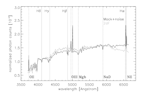
Figure 2 shows the mean spectrum for the 2dF and mock+noise catalogues, obtained by simply averaging the photon counts in each wavelength bin for all the galaxies in the ensemble. The mean spectra for the observed and mock catalogues are seen to be similar. The magnitude limit that we have chosen is such that our ensembles are dominated by fairly bright, moderately star-forming spiral galaxies, and the mean spectra show familiar features such as the 4000 Å break, the Balmer series, and metal lines such as OII and OIII. One can see that the 2dF spectrum appears to bend downwards relative to the models towards both ends of the wavelength range. This may be due to an inaccurate correction for the response function, as discussed above.
4 Results

We now apply the IB algorithm to both the 2dF and the mock data. Recall that our algorithm begins with one class per galaxy, and groups galaxies so as to minimize the loss of information at each stage. Figure 3 shows how the information content of the ensemble of galaxy spectra decreases as the galaxies are grouped together and the number of classes decreases. In the left panel, we show the ‘normalized’ information content as a function of the reduced complexity , where is the number of galaxies in the ensemble and is the number of classes. One may think of this as the fraction of information about the original ensemble that would be preserved if we threw away all the individual galaxies and kept only the representative spectra of the classes. Remarkably, we find that if we keep about five classes, about and percent of the information is preserved for the mock and mock+noise simulations, respectively. This indicates that the wavelength bins in the model galaxy spectra are highly correlated. This may not seem very surprising, since many of the spectral features arise from the same stellar physics. For example, emission lines will be stronger in a galaxy with significant recent star formation, and the whole sequence of metal absorption lines will be deeper for a galaxy with an old stellar population or a high metallicity. However, if we keep in mind that each of our model galaxies has a very complex star formation history and is therefore comprised of stars with a distribution of ages and metalicities, and is affected differently by dust extinction, this result may seem somewhat more surprising.
In contrast with the mock samples, for the 2dF catalogue, only about percent of the information is preserved by five classes. Thus the wavelength bins in the real spectra are also highly correlated, but not to the same degree as the model spectra. This is unlikely to be solely due to the effect of noise. Adding noise to the mock catalogues does change the curve in Figure 3 (left panel), bringing it closer to the 2dF curve, but the effect is not large enough to explain the whole discrepancy, and moreover the shapes of the mock+noise and 2dF information curves are still different. We also see that the ‘absolute information’ for 2dF (right panel of Figure 3) is much higher than for the mock samples. This discrepancy may be partially due to the influence on the real spectra of more complicated physics than what is included in our simple models. It could also be due to systematic observational errors (see Section 3.1). We are in the process of attempting to model these systematic errors in detail to better understand this result.
The information curves are not sensitive to the number of galaxies used in the analysis. When we take a random subset of 2611 galaxies out of the 2dF sample (to make it identical to the number of galaxies in the mock sample), the differences in the information curve w.r.t the full 2dF set are minor. We also experimented with the ‘Euclidean’ algorithm (see Section 2.3) for both the mock and 2dF data. We find that for the mock data, the Euclidean algorithm produces nearly indistinguishable results from our fiducial algorithm, however, for the 2dF data, the difference between the two is more significant. The full IB algorithm preserves more information for any given number of classes and is therefore superior. This suggests that the Euclidean-type algorithms may be sufficient for certain problems, but inadequate for more complex data.
4.1 The IB Classes
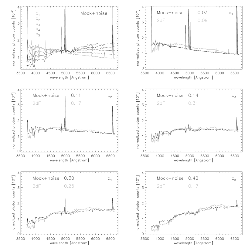
For the remainder of this paper, we present the results obtained for five classes. 666We note that galaxy images can be reliably classified by morphology into no more than 7 or so classes (e.g. Lahav et al. 1995; Naim et al. 1995a) Figure 4 shows the representative spectra for these five classes for both the 2dF and mock+noise catalogues. The corresponding five spectra for the noise-free mock data were very similar to the mock+noise spectra shown. We ‘matched’ each of the classes obtained for the 2dF data with one from the mock+noise data by minimizing the average ‘distance’ between the pairs. The classes are then ordered by their mean colour. Note that the five classes produced by the algorithm appear similar for both catalogues — there was certainly no guarantee that this would be the case.
It is also interesting to examine the relative fractions of galaxies in each class, , for the observed and mock catalogues. These values are given on the appropriate panels of Figure 4. There is a partial agreement between the weights of the matched classes for the 2dF and mock+noise catalogues (although particularly for and , the agreement is not very good). We might hope that this could provide a way to improve the physics included in the models by constraining the relative composition of different types of galaxies in more detail than was previously possible. However, we find that adding noise to the mock catalogues causes some galaxies to “jump” to different classes, thus changing the relative fractions. When we add noise at the level of the 2dF data as described previously, percent of the galaxies are assigned to a different class than in the noise-free case. Of these, the great majority ( percent) are assigned to adjacent classes (i.e. ). We note these results are for the ‘hard’ version of the algorithm. We expect the ‘soft’ version of the algorithm to be less sensitive to noise.
We are also concerned that some of the noticeable discrepancy in the shape of the mean spectra of the 2dF classes and those of the synthetic galaxies (also noted in the comparison of the mean spectra, Figure 2) may be due to systematic observational effects such as inaccurate modelling of the response function. In the future we hope to be able to model and correct for these effects.
More generally, we can see that the algorithm is sensitive to the overall slope (or colour) of the spectrum, and also to the strength of the emission lines. The classes clearly preserve the familiar physical correlation of colour and emission line strength; the five classes form a sequence from , which has a blue continuum with strong emission lines, to , with red continuum with no emission lines 777Recall that the order of the classes as produced by the algorithm is arbitrary, and we have placed them in this sequence by hand, but the correlation of colour and emission line strength within the classes is produced by the algorithm with no help from us. Already, we may form the impression that the algorithm has classified the galaxies in a way that is reminiscent of conventional spectral classes. It may be interesting to compare the mean spectrum of with the spectrum of the Sm/Irr galaxy NGC449, and with the Sa galaxy NGC775 from Figure 2a of Kennicutt (1992). Apparently, the class corresponds to late type galaxies (Sm/Irr) and to early types (Sa-E).
4.2 Correlation of the IB Classes with Physical Properties

In order to gain a better understanding of the IB classes, we now use the noise-free mock catalogue and investigate the physical properties of the galaxies in each class as given by the same models that we use to produce the spectra. The parameters that we chose to investigate are: colour, the ratio of the present to past-averaged star formation rate (Kennicutt b-parameter, ; Kennicutt 1983), the ratio of the mass of the bulge to the total stellar mass of the galaxy (), the fraction of the total baryonic mass in cold gas (), the mean mass-weighted stellar age and metallicity, the internal velocity dispersion or circular velocity , and the B-band absolute magnitude .
Figure 5 shows the trends of these physical parameters with class number. The strongest dependence is of colour and present-to-past-averaged star formation rate . Class contains blue galaxies that are forming stars at rates that are one to two orders of magnitude higher than the average over their past history. As one moves towards , galaxies are redder and formed a larger fraction of their stars in the past. This is consistent with the observed strong correlation of the Kennicutt b-parameter with colour and morphological type in nearby galaxies (Kennicutt et al. 1994). For reference, note that the mean colour for Sm/Irr galaxies in the local Universe is , for Sbc-Sc , for Sab-Sb , for S0a-Sa , and for E-S0 (Roberts & Haynes 1994). From the colours alone, we might guess that galaxies in and are starburst galaxies, galaxies in are Sm-Irr, corresponds to Sb/Sbc and to Sa/S0/E. This bolsters our initial impression based on the visual appearance of the spectra. Weaker trends are visible in other properties: the sequence - shows an increasing B/T ratio, as expected, but with a large scatter within each class. There is quite a large scatter in the observed correspondence between morphological T-type and bulge-to-total ratio, but values of are typical of very early-type spirals (Sa) or lenticular galaxies (cf. Simien & de Vaucouleurs 1986). Weak trends are also visible in the mean stellar age and metallicity and the internal velocity dispersion: as we move from –, galaxies tend to be older, more metal rich, and more massive. This is in accord with the observed trends of these quantities with morphological type (cf. Roberts & Haynes 1994) and the trends we have noted previously.
We find no trend of dust extinction with the IB classes, probably because we have assumed that dust extinction attenuates the emission lines and the continuum by the same factor. Therefore the dust only changes the overall colour of a galaxy, but does not affect the ratio of emission or absorption lines to continuum.
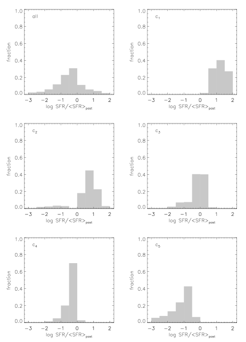
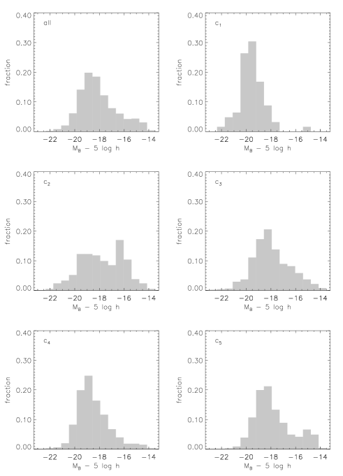
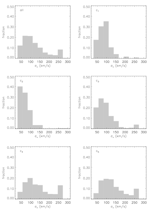
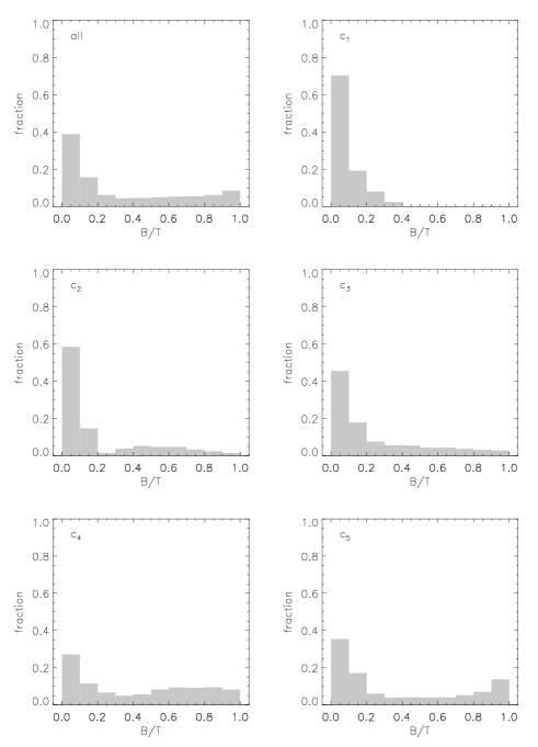
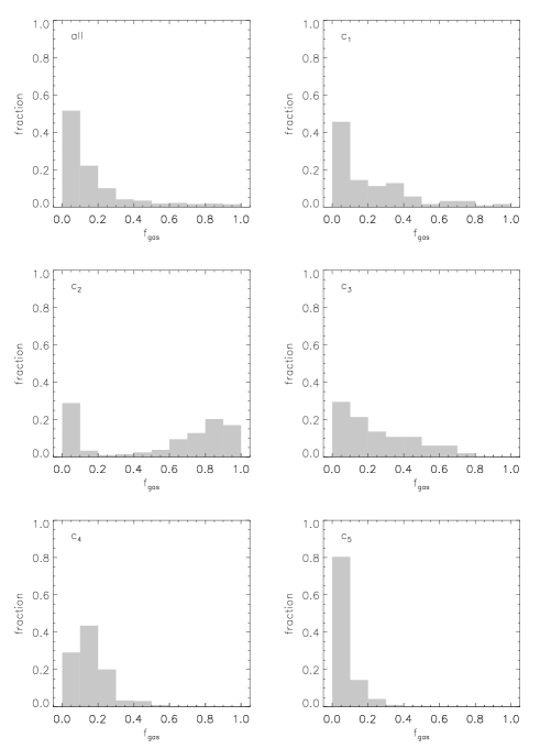
We investigate the composition of the classes in more detail by examining the distributions of some of the physical parameters for the different classes. In each of figures 6-10, in the upper left-most panel we show the distribution of the relevant physical parameter for the whole ensemble of model (noise-free) galaxies. In the other five panels we show the distributions for the galaxies in each class separately. Figure 6 shows the distribution of Kennicutt’s parameter (ratio of present-to-past-averaged SFR). This parameter shows a particularly strong correlation with the IB class assignment, although the distributions show significant overlap. Figure 7 shows the distribution of B-band absolute magnitudes. Class contains an excess of bright galaxies, whereas and to a lesser extent contain excesses of faint galaxies compared to the overall distribution. Figure 8 shows the distribution of the internal velocity dispersion of the galaxies, a measure of the dynamical mass of the galaxy. Here we note the curious fact that the distribution is skewed towards small galaxies in -, and towards large galaxies in -. This suggests that galaxies in , which are preferentially bright and with small mass are starburst galaxies. We return to this point later.
In Figure 9, we see that is entirely composed of disk-dominated galaxies (). The classes become progressively more skewed towards larger , bulge-dominated galaxies as we move towards . However, despite the fact that we noted that the spectral appearance, colors and star formation rates of galaxies in - are typical of observed galaxies with bulges (Sb-E), in the models these classes contain a significant fraction of nearly pure disks (). This may be an indication that the connection between star formation and morphology is not being modelled properly.
The distribution of gas fraction is shown in Figure 10. In , there are quite a lot of galaxies with fairly low gas fractions. This is somewhat in conflict with our previous association of this class with late-type galaxies, but perhaps not if most of these galaxies have experienced a very recent starburst which would have tended to consume the gas supply very quickly. The class is highly skewed towards high gas fractions, but with some objects with low gas fractions — perhaps this class is composed of a combination of post-starburst galaxies and quiescent, gas rich galaxies. Classes - are composed solely of rather gas-poor galaxies, confirming that these galaxies have probably been evolving passively, with little new star formation.
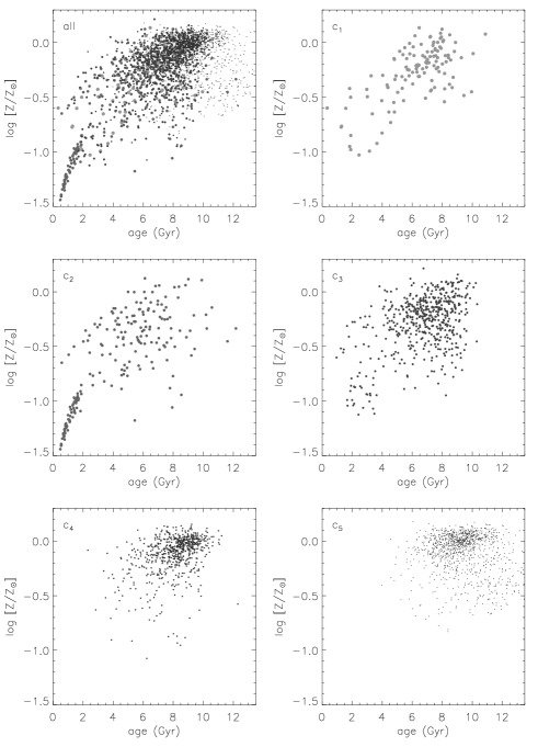
It is also useful to see where the classes are located in the two-dimensional space of pairs of the physical parameters. In the following figures, we once again show the entire ensemble in the upper left panel, and the breakdown by class in the other five panels. Figure 11 shows the mean stellar metallicity of galaxies as a function of their mean stellar age. We see that there is a weak trend, with a large scatter, between these two quantities in our models. This trend is stronger for classes -, and becomes mostly washed out for -. Galaxies in - also tend to have higher metallicities for their age than galaxies in -. As applied here, the algorithm suffers from the familiar age-metallicity degeneracy. However, an alternative way of applying the algorithm (by asking it to preserve the maximum information about a particular physical parameter, e.g. age or metallicity) may prove to be effective for this problem. We intend to pursue this in future work.
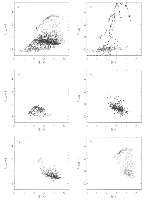
We also examine how the classes inhabit a classical colour-colour diagram. Figure 12 shows the far-UV/optical (1500 Å-B) and optical/near-IR (B-K) colours. Recall that the spectra that we provided to the IB algorithm did not contain any information about the far-UV (1500 Å) or near-IR (K-band) magnitudes. Galaxies in have a narrow range of very blue UV-B colours but a broad range of B-K colours. The shape and orientation of this clump changes as we move from -. The lines on the top right panel show the tracks for instantaneous bursts of fixed age and metallicity from the Bruzual & Charlot models (see figure caption). This illustrates the complex manner in which both age and metallicity determine the location of galaxies in this diagram.
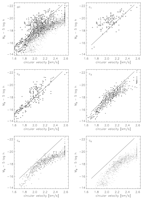
Figure 13 shows the absolute B-magnitude as a function of circular velocity. This is essentially what is usually known as the Tully-Fisher (TF) relation, although it should be noted that our model magnitudes contain the effects of dust extinction, unlike observed TF samples where at least the effects of inclination are generally removed. Nor have we made any cut on morphology or gas fraction in the models. This is why the slope and scatter of the relation plotted look so different from the usual TF relation. It was shown in SP that when the above effects are accounted for, we obtain reasonable agreement with the observed zero-point, slope, and scatter of the I-band TF relation in these models. The interesting thing to note is the way the classes cut the two-dimensional space of this diagram. Galaxies in lie at preferentially bright magnitudes for their velocity/mass (i.e., they are starbursts), whereas galaxies in lie at preferentially faint magnitudes for their velocity/mass. An increasing curvature of the relation is also seen from to . The progressive offset of the TF relation with varying Hubble type is recognized (Burstein et al. 1997) but not very well understood. This result offers a hint as to its origin, and also suggests that the familiar observed TF relation and its small scatter may be a special feature of the particular type of galaxies that are generally selected for these samples.
5 Comparison with PCA
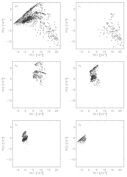
PCA has previously been applied to data compression and classification of spectral data of stars (e.g. Murtagh & Heck 1987; Bailer-Jones et al. 1997), QSO (e.g. Francis et al. 1992) and galaxies (e.g. Connolly et al. 1995a; Folkes, Lahav & Maddox 1996; Sodre & Cuevas 1997; Galaz & de Lapparent 1997; Bromley et al. 1998; Glazebrook, Offer & Deeley 1998; Ronen et al. 1999; Folkes et al. 1999). As we noted earlier, while PCA operates as an efficient data compression algorithm, it is purely linear, based only on the variance of the distribution. PCA on its own does not provide a rule for how to divide the galaxies into classes. 888 For example, in Folkes et al. (1999) the classification was done by drawing lines in the plane using training sets. One training set was based on visual inspection of the spectra by a human expert. This led to classification which is more sensitive to emission and absorption lines, rather than to the continuum (which is affected by observational problems). It is therefore interesting to see where the IB classes reside in the space of the PC components. The PC eigenvectors are defined in the usual way (see the above references for more details), and the projections of the (noiseless) model spectra onto the first two components of this basis (PC1 and PC2) are shown in Figure 14. The overall pattern reminds the one seen in the models of Ronen et al. (1999) and in the 2dF data (Folkes et al. 1999), but note that the PC eigenvectors are different for every data set. We note that our 5 IB classes form fairly well-separated “clumps” in PC1-PC2 space, and that to a first approximation, the IB classification is along PC1. This highlights the need to correct properly the artifacts due to optics so that the continuum (colour) and hence PC1 can be determined accurately. The PC-space of the IB clumps looks quite different from the partitioning (based on training sets) given in Folkes et al. (1999). It has been shown (Ronen et al. 1999) that PC1 and PC2 are correlated with colour and emission line strength, and the sequence from - is again sensible in this context.
6 Discussion
Unsupervised classification methods are generally used to obtain efficient representation of complex data. One can identify two general classes of techniques for achieving this goal, geometrical and statistical. Geometrical methods begin by an embedding of the data in a high dimensional, usually Euclidean, space, and then searching for a low dimensional manifold that captures the essential variation of the data. The simplest of such methods is PCA, which provide a linear projection of the data. PCA can be generalized to more powerful linear projections, e.g. projection pursuit (Friedman and Tukey 1974) or to nonlinear projections that maximize statistical independence, such as Independent Component Analysis (ICA; Bell and Sejnowski 1995). These methods provide a low dimensional representation, or compression, in which one might hope to identify the relevant structure more easily. Another approach of identifying classes of objects in a parameter-space (based on a training set) is by utilising Artificial Neural Networks (e.g. used for morphological classification of galaxies; Naim et al. 1995b; Lahav et al. 1996).
Statistical methods assume that the data is sampled from an underlying distribution with some knowledge of its parametric structure. Finding the structure of data amounts then to the estimation of the unknown parameters of the distribution. Such methods include the familiar Gaussian mixture estimation and similar vector quantization techniques. Modern formulation of many of the statistical as well as geometrical methods is based on information maximization principles for finding either efficient compression or statistical independence among the features.
Other compression methods have also been proposed for our problem, e.g. by starting with standard Maximum Likelihood desired parameters (e.g. age) and utilising the Fisher information matrix to define a set of optimal axes (Heavens, Jimenez & Lahav 2000).
The information bottleneck method presented here provides a new statistical approach to structure extraction. Unlike all other techniques it aims directly at the problem of the extraction of the relevant structure or features, where the relevance is determined through the information on another, carefully chosen, variable. The goal of the method is well defined and objective, with natural information theoretical figures of merit. It is superior to both geometric and statistical methods since it makes no model-dependent assumptions on the data origin, nor about the similarity or metric among data points.
An important issue, common to most unsupervised classification methods, is model order estimation: what is the correct number of classes? This question is closely related to the sampling noise issue — the obtained classes should not be sensitive to the specific sample, thus should be robust to sampling noise. This criterion can be checked, using techniques such as cross-validation, in most clustering algorithms including ours. Yet it is important to emphasize that the “true” or “correct” number of classes may be an ill-defined quantity for real data sets. The number should be determined by the desired resolution, or preserved information in our case.
We have shown how the IB algorithm can be used to classify galaxy spectra in a principled and objective way. The number of distinct classes is specified by an acceptable degree of information loss. We have applied the algorithm to a subset of spectra from the ongoing 2dF redshift survey, and to a mock-2dF catalogue of synthetic spectra obtained from semi-analytic hierarchical (CDM) models of galaxy formation.
We find that five classes preserve about 50 percent of the information about the ensemble of 2dF spectra. The same number of classes preserves 85 percent of the information about the model spectra in the absence of Poisson noise. When noise is added to the models with S/N comparable to the 2dF data, five classes preserve 75 percent of the information.
Examining the mean spectra of the five classes produced by our algorithm, we first see that there is a good matching between the five average spectra obtained for the mock data and the five average spectra obtained for 2dF. It is also apparent that these spectra form a sequence from blue galaxies with strong emission lines to red galaxies with strong absorption lines and no emission lines. This corresponds well with the general approach usually followed in more subjective spectral classification methods (i.e. “by eye”).
For the model galaxies, we also show that the classes form sequences in several physical quantities, such as the present-to-past-averaged star formation rate (Kennicutt parameter), morphology (as represented by the ratio of bulge-to-total stellar mass), and stellar mass/velocity dispersion. Since the spectra obviously do not contain any of this information directly, the existence of these correlations (which are in accord with known observational correlations among the physical parameters studied) seems to indicate two things. First, that the physics used to create the model galaxies is fairly sensible. Second, and more novel, grouping the galaxies in a way that formally preserves the information with respect to the spectra (as our method does), discovers interesting physical correlations.
Again for the models, we find that the classes occupy different parts of bivariate diagrams in pairs of the physical parameters, such as age vs. metallicity, color-color, and luminosity vs. circular velocity (Tully-Fisher). These results may hint at important clues as to how to constrain the star formation histories of different types of galaxies and the physical origin of these sorts of relationships.
We compare our results with those of a Principal Component Analysis. We find that the classes produced by the IB algorithm form fairly well-defined clumps in the PC1-PC2 space (the projections onto the first two principle component eigenvectors).
We conclude that this method provides a way to classify galaxies that is fully automated and objective, yet is related to the physical properties of galaxies and the intuition that astronomers have built up over the years using more subjective methods. A further advantage is that this method can be applied in exactly the same way to observations and models such as the ones investigated here, allowing comparisons between theory and observations to be made on the same footing. We intend to apply the algorithm to the full set of galaxy spectra obtained from the 2dF redshift survey. Obvious applications are then to study the spatial clustering of different classes and relative biasing among them, and luminosity functions divided by class. If spectra with adequate signal-to-noise can be obtained, the same method could be applied to high redshift spectra to study the evolution with redshift of different types of galaxies.
7 acknowledgment
We thank S. Folkes, D. Madgwick, A. Naim, S. Ronen, and the 2dFGRS team for their contribution to the work presented here. This research was supported by a grant from the Ministry of Science, Israel.
References
- [1]
- [2] Axze’l J., Daro’czy Z., 1975, On Measures of Information and Their Characterization, Academic Press, New York
- [3] Bailer-Jones C.A.L., Irwin M., Gilmore G., von Hippel T., 1997, MNRAS, 292, 157
- [4] Barnes J., Hernquist L., 1992, ARA&A, 30, 705
- [5] Bell A.J., Sejnowski T.J., 1995, Neural Computation, 7, 1129
- [6] Benitez N., 1999, ApJ, in press (astro-ph/9811189)
- [7] Bialek W., Nemenman, I., Tishby, N., 2000, NECI Technical Report, Neural Computation, in press
- [8] Bromley B.C., Press W.H., Lin H., Kirshner, R.P, 1998, ApJ, 505, 25
- [9] Bruzual G., Charlot S., 1993, ApJ, 405, 538
- [10] Bruzual G., Charlot S., 1996, Galaxy Isochrone Synthesis Spectral Evolution Library, Multi Metallicity Version (GISSEL96)
- [11] Burstein D., Bender R., Faber S., Nolthenius R., 1997, AJ, 114, 1365
- [12] Cole S., Aragón-Salamanca A., Frenk C., Navarro J., Zepf S., 1994, MNRAS, 271, 781
- [13] Colless M.M., 1998, in Morganti R., Couch W.J., eds, ESO/Australia workshop, Looking Deep in the Southern Sky, Springer Verlag, Berlin p. 9
- [14] Connolly A.J., Szalay A.S., Bershady M.A., Kinney A.L., Calzetti D., 1995, AJ, 110, 1071
- [15] Cover, T.M., Thomas, J.A. 1991, Elements of Information Theory, John Wiley & Sons, New York
- [16] El-Yaniv R., Fine S., Tishby N., 1997, in Jordan, M., Kearns, M., Solla, A., eds., Advances in Neural Information Processing Systems (NIPS), Vol 10, p. 465
- [17] Fioc M., Rocca-Volmerange B., 1997, A&A, 326, 950
- [18] Folkes S.R., Lahav O., Maddox S.J., 1996, MNRAS, 283, 651
- [19] Folkes S.R., et al. 1999, MNRAS, 308, 459
- [20] Francis P.J., Hewett P.C., Foltz G.B., Chaffee, F.H., 1992, ApJ, 398, 476
- [21] Friedman J.H., Tukey J.W., 1974, IEEE Trans. Comput. C(23), 881
- [22] Fukugita M., The Sloan Digital Sky Survey, in proceedings of IAU, Kyoto, 1997, Highlights of Astronomy, vol. 11
- [23] Galaz G., de Lapparent V., 1998, A&A, 332, 459
- [24] Glazebrook K., Offer A.R., Deeley K., 1998, ApJ, 492, 98
- [25] Guiderdoni B., Rocca-Volmerange, B., 1987, A&A, 186, 1
- [26] Gunn J.E., Weinberg D.H., 1995, in Maddox S.J., Aragón-Salamanca, A., eds., Wide Field Spectroscopy and the Distant Universe, World Scientific, Singapore, p. 3
- [27] Heavens A., Jimenez R., Lahav, O., 2000, MNRAS, submitted (astro-ph/9911102)
- [28] Humason, M.L., 1936, ApJ, 83, 18
- [29] Kauffmann G., White S., Guiderdoni B., 1993, MNRAS, 264, 201
- [30] Kennicutt R.C. 1983, ApJ, 272, 54
- [31] Kennicutt R.C. 1992, ApJS, 388, 310
- [32] Kennicutt R.C., Tamblyn P., Congdon, C.W., 1994, 435, 22
- [33] Lahav, O. et al., 1995, Science, 267, 859
- [34] Lahav, O., Naim, A., Sodre, L., Storrie-Lombardi, M.C., 1996, MNRAS, 283, 207
- [35] Lin J., 1991, IEEE Transactions on IT, 37, 1, 145
- [36] Morgan, W.W, Mayall, N.U., 1957, PASP, 69, 291
- [37] Murtagh F., Heck A., 1987, Multivariate Data Analysis, Reidel, Dordrecht
- [38] Naim A., et al., 1995a, MNRAS, 274, 1107
- [39] Naim A., Lahav, O., Sodre, L., Storrie-Lombardi, M.C., 1995b, MNRAS, 275, 567
- [40] Pereira F., Tishby N., Lee L., 1993, in The 30th Annual Meeting of the Association for Computational Linguistics, p. 183
- [41] Pierce M., Tully, B., 1992, ApJ, 387, 47
- [42] Roberts M., Haynes, M., 1994, ARA&A, 32, 115
- [43] Ronen S., Aragon-Salamanca A., Lahav O., 1999, MNRAS, 303, 284
- [44] Rose K., 1998, IEEE Transactions on IT, 86, 11, 2210
- [45] Shanon C.E., 1948a, The Bell System Technical Journal, 27, 379
- [46] Shanon C.E., 1948b, The Bell System Technical Journal, 27, 623
- [47] Sheth R.K., Tormen G., 1999, MNRAS, 308, 119
- [48] Simien F., de Vaucouleurs G., 1986, ApJ, 302, 564
- [49] Slonim N., Tishby N., 1999, Neural Information Processing Systems (NIPS-99)
- [50] Slonim N., Tishby N., 1999, Proc. of Neural Information Processing Systems (NIPS-99)
- [51] Slonim N., Tishby N., 2000, 23d Annual International ACM SIGIR Conference on Research and Development in Information Retrieval, in press
- [52] Sodré L. Jr., Cuevas H., 1997, MNRAS, 287, 137
- [53] Somerville R.S., 1997, PhD Thesis, Univ. California, Santa Cruz
- [54] Somerville R.S., Primack, J.R., 1999, MNRAS, 310, 1087
- [55] Somerville R.S., Primack J.R., Faber S.M., 2000, MNRAS, submitted
- [56] Somerville, R.S., Bullock J., Mac Minn D., Primack J.R., 2000b, in prep.
- [57] Somerville R.S., Kolatt T., 1998, MNRAS, 305, 1
- [58] Tishby N., Pereira F.C., Bialek W., 1999, Proc. of the 37th Allerton Conference on Communication and Computation