Wide-field imaging at mid-infrared wavelengths :
reconstruction of chopped and nodded data

Abstract

Ground-based astronomical observations at thermal infrared wavelengths ($\lambda\geq 2.4~{}\mu$m) face the problem of extracting the weak astronomical signal from the large and rapidly variable background flux. The observing strategy most commonly used, the so-called “chopping and nodding” differential technique, provides reliable representations of the target uniquely in the case of compact sources while extended and complex sources can be easily distorted by their negative counterparts. A restoration method, designed to remove the negative values and to provide reliable representations of extended sources, has been proposed by us in two previous papers and validated on simulated images (Bertero et. al 1998, 1999). In this paper we apply our algorithm to real images taken at UKIRT telescope with the MPIA camera MAX. We show that the algorithm successfully removes the distortions due to the negative counterparts and, in addition, provides noise reduction. In several cases an enlargement of the field is obtained, in the sense that the restored larger image provides reliable information on the source structure outside the central field of view. The restorations may be affected by artifacts, whose origin can be predicted theoretically. We suggest and demonstrate computational and observational procedures for their reduction. Once combined with the proper observing strategies, our inversion method can provide a viable solution to the problem of deep imaging of extended sources with large ground-based telescopes.

1 Introduction

Ground-based astronomical observations at infrared (IR) wavelengths can only be performed through a limited number of atmospheric windows (Thomas & Duncan (1993)). Under the best observing conditions, the atmospheric transmission closely approaches $\tau\simeq 1$ $(100\%)$ within a few narrow spectral intervals, but typical broad-band values are significantly smaller. Even at excellent sites like Mauna Kea, the median transmission in the 8–13 $\mu$m window (N band) is $\tau\simeq 0.85$ (see e.g. the UKIRT web page).

Besides reducing the number of source photons reaching the detector, the atmosphere absorbs and thermally re-radiates isotropically a corresponding fraction of energy coming from the space and especially from the ground. In a first approximation, the atmosphere can be conveniently regarded as a gray-body radiator with emissivity $\epsilon=1-\tau$ (Kirchoff’s law) and temperature $\approx 230-250$K. The corresponding photon flux, peaking at 10 $\mu$m, is huge compared to the celestial background, e.g. $\approx 10^{6}$ times higher than the zodiacal background at 10$\mu$m. The telescope itself also adds an important contribution to the background flux. Opaque surfaces within the optical beam (secondary mirror spiders, primary mirror cell and central obstruction) are near-blackbody radiators, whereas the mirrors themselves and the other warm optics, partially reflecting or transmitting, are gray-body emitters. Proper opto-mechanical design and regular cleaning of the optical surfaces can reduce the emissivity budget of a telescope to a few percents. Still, the total background flux at 10$\mu$m within a 1$\mu$m bandpass remains of the order of $10^{9}$ photons s^-1 m^-2 arcsec^-2, roughly corresponding to an astronomical source of magnitude $N\approx-3.0$.

Today, it is possible to routinely detect at 10$\mu$m point sources some 12 magnitudes fainter than the background per square arcsecond in a few minutes with 3–4 m telescopes and, in particular, UKIRT (Robberto & Herbst (1998)). To attain these performances special observing techniques must be adopted, but they are not without drawbacks.

If $x,y$ are angular coordinates in the sky, the signal $s_{P}$ coming from the direction $\{x,y\}$ at time $t$ and detected on the corresponding pixel $P$ of the detector can be expressed as:

$$s_{P}=T_{P}[f(x,y)+a(x,y,t)]$$ (1)

where $f$ is the unknown brightness distribution of the celestial source and $a$ is the large and time-variable thermal background flux. The transfer function of the detection system $T_{P}$ includes the collecting area of the telescope, the field of view of each individual pixel and the overall optical transmission. Under the conditions described by equation (1) it is clear that a small error in the estimate of $a$ will dramatically affect the extraction of the signal $f$.

The background $a$ can be obtained in principle by pointing the telescope to a sky area close to the region of interest at a time $t^{\prime}$ close to $t$. Assuming that this area corresponds to a shift $\Delta$ in the $y$ coordinate, then the new signal $s^{\prime}_{P}$ detected at the pixel $P$ is

$$s_{P}^{\prime}=T_{P}[f(x,y+\Delta)+a(x,y+\Delta,t^{\prime})].$$ (2)

If the sky area close to that of interest is empty, i.e. $f(x,y+\Delta)=0$, and close enough in space and time that the background is approximately the same, i.e. $a(x,y+\Delta,t^{\prime})\simeq a(x,y,t)$, then by subtracting equation (2) from equation (1) one can obtain $T_{P}f(x,y)$. In this way the signal can be known within the accuracy of the system response.

In practice, the telescope must sample the two areas fast enough that the temporal fluctuations of $a$ are small. The actual frequency depends on various factors: observing wavelength, weather conditions, telescope location etc., but is typically faster than a few Hz (Kaeufl et al. (1991)). Whereas it is, in general, impossible to repeatedly move a telescope at these frequencies, a single optical element can be rapidly “chopped” between two slightly different positions, allowing the detector to see two nearby sky areas. To minimize pupil motion at the cold stop, the secondary mirror of the telescope is often undersized (so it becomes the exit pupil of the tescope) and modulated. This classic technique is called secondary chopping and the quantity $\Delta$ is the chopping throw or chopping amplitude. Given a certain amplitude, the maximum chopping frequency is constrained by the settling time of the secondary mirror structure, typically of the order of 20-50 milliseconds.

Even neglecting the efficiency loss due to the time spent observing the sky and waiting for the secondary mirror to settle, this method presents important limitations. First, by moving an optical element of the system, the detectors look through different parts of the optical system (including high emissivity surfaces like central obstruction, mirror edges, spiders, etc.). Therefore, the resulting differential image turns out to be affected by a residual background variation due to the thermal differences between the two beams. In other words, chopping is equivalent to rapid switching between two different telescopes, one $(A)$ for the source and another ${(B)}$ for the sky. We will denote by $\Delta a_{AB}$ the residual difference between the corresponding background patterns. Second, for optical and mechanical reasons the typical chopping throws are usually less than 60 arcseconds, possibly much less for 8-m class telescopes. If the source is extended enough, and/or if the telescope is sensitive enough, it can be $f(x,y+\Delta)\neq 0$. Therefore, the subtraction of equation (2) from equation (1) gives:

$$\Delta s_{A}=s_{P}-s_{P}^{\prime}=T_{P}[f(x,y)-f(x,y+\Delta)+\Delta a_{AB}]$$ (3)

where with $\Delta s_{A}$ we indicate that the source has been observed with the ${(A)}$ beam.

To remove the term $\Delta a_{AB}$, the so-called beam-switching or nodding technique is applied: the telescope is pointed to a different point on the sky, so that the source will be observed with the ${(B)}$ beam (this maximizes the signal-to-noise ratio). In our notation, the telescope is shifted by $-\Delta$ arcseconds in the $y$ coordinate. In this way, at the pixel $P$ the signal $s_{P}^{\prime\prime}$ is obtained and, repeating the entire sequence, the result is:

$$\Delta s_{B}=s_{P}^{\prime\prime}-s_{P}=T_{P}[f(x,y-\Delta)-f(x,y)+\Delta a_{AB}].$$ (4)

Subtracting equation (4) from equation (3), one gets the so-called chopped and nodded image:

$$g_{\Delta}(x,y)=\Delta s_{A}-\Delta s_{B}=T_{P}[-f(x,y-\Delta)+2f(x,y)-f(x,y+\Delta)],$$ (5)

i.e. an image which is independent of the atmospheric background and telescope thermal pattern. If the source brightness distribution is sufficiently compact, i.e. if $f(x,y-\Delta)=f(x,y+\Delta)=0$, then the problem of extracting $f(x,y)$ is solved. Otherwise a method for recovering $f(x,y)$ from the image $g(x,y)$ is required.

As already pointed out (Beckers (1994), Kaeufl (1995)), there is little doubt that such a method is becoming highly needed. The continuous technological developments both in the field of infrared array detectors, which allow one to reach the natural background-noise limited performances for broad-band imaging, and of large telescope engineering, with approximately a dozen of 8-meter class telescopes in operation or in an advanced construction phase, are greatly improving the sensitivity of thermal infrared instrumentation. Because giant telescopes have smaller pixel scales and have limited chopping amplitudes, the case $f(x,y-\Delta)=f(x,y+\Delta)=0$ cannot be regarded any more as the typical one so that the $f(x,y\pm\Delta)$ components of the scene appear as negative signals in the final image (see equation (5)). In such cases a restoration method is required to obtain, in the general case of a structured astronomical object, an image free from negative values and reproducing, as far possible, the correct intensity distribution within the source.

In (Bertero et al. (1998), hereafter BBR98) a preliminary investigation of this problem has been performed and it has been found that an iterative regularization method, the so-called projected Landweber method, can provide a viable solution. The method provides a positive restoration of the chopped and nodded image by removing completely the negative counterparts of compact and extended sources. The mathematical properties of the problem, as well as the validation of the method by means of simulated images, have been presented in (Bertero et al. (1999), hereafter BBDR99).

In Section 2 of this paper we outline the mathematical model we use for describing the chopping and nodding technique, we discuss the various kinds of instrumental errors which are not included in the mathematical model and we describe the iterative restoration method we propose. In addition, we discuss the criteria for stopping the iterations, the so-called stopping rules, which are an important issue for the correct use of the method. Finally, we describe three types of artifacts and show how they are related to the mathematical properties of the problem.

In Section 3 we apply the method to real astronomical images taken at the UKIRT telescope. We show that not only the effects of the negative counterparts of the sources are successfully corrected, but also the noise is reduced, if the number of iterations is properly chosen. We indicate the stopping rule which is the most convenient at the present stage of our analysis. We also show that an enlargement of the field is possible, even if the restoration outside the field is, in general, less accurate than within. Moreover our restored images provide several examples of the artifacts described at the end of Section 2.

In Section 4 we propose three computational and observational procedures for the reduction of the artifacts, and we show that by applying these methods it is possible to produce mid-IR images of extended sources with high accuracy and sensitivity. Finally, in Section 5 we summarize our results and provide a few practical hints on the instrument alignment at the telescope that should permit the algorithm to produce the optimal results.

2 An outline of the restoration method

We take, for simplicity, $T_{P}=1$ in equation (5). Then by computing the Fourier transform of both sides we get

$$\hat{g}_{\Delta}(\omega_{x},\omega_{y})=4sin^{2}({1\over 2}\Delta\omega_{y})\hat{f}(\omega_{x},\omega_{y})$$ (6)

where $\omega_{x},\omega_{y}$ are the spatial frequencies associated with the variables $x,y$ respectively. As already observed by Beckers (Beckers (1994)), equation (6) shows that the chopped and nodded image does not contain information about $\hat{f}(\omega_{x},\omega_{y})$ at the frequencies $\omega_{y,k}=2\pi k/\Delta$ $(k=0,\pm 1,\pm 2,\cdots)$, so that the chopping and nodding technique looks equivalent to the application of a Fourier grating to the original object. However, the Fourier transform of the measured data is not zero at these frequencies because they are contaminated by noise (Kaeufl (1995)). As a consequence, the restoration of $\hat{f}(\omega_{x},\omega_{y})$ cannot be obtained by dividing the Fourier transform of the chopped and nodded image by the factor $sin^{2}(\Delta\omega_{y}/2)$.

In general Fourier based methods cannot be used for this problem because the functions $f$ and $g$ are not defined on the same domain. If the region of interest corresponds to the interval $[0,Y]$ in the y-variable, then the image $g_{\Delta}(x,y)$, defined on this interval, receives contributions from the values of $f(x,y)$ on the broader interval $[-\Delta,Y+\Delta]$. A method, able to restore $f(x,y)$ on this interval, will provide an enlargement of the field.

Let us assume that the detector plane is partitioned into $N\times N$ pixels, with size $\delta\times\delta$, labeled with an index $j$ corresponding to the columns and an index $m$ corresponding to the rows of the array. Since the chopping is in the $y$-direction, it is parrallel to the columns of the array. Further we assume that the chopping amplitude $\Delta$ is a multiple of the sampling distance $\delta$, i.e. $\Delta=K\delta$ with $K$ integer and smaller than $N$. Most of the images we consider are $128\times 128$ and $K$ is typically (but not necessarily) betwen 30 and 50.

Let $g_{j,m}$ and $f_{j,m}$ be the samples of $g(x,y)$ and $f(x,y)$ respectively. For each $j$ the values $g_{j,m}$, with $m$ running from $1$ to $N$, form a vector of length $N$ which will be denoted by ${\bf g}_{j}$. It receives contributions from $N+2K$ values $f_{j,m}$, with $m$ running from $1$ to $N+2K$, which form a vector of length $N+2K$, denoted by ${\bf f}_{j}$ . The components of ${\bf f}_{j}$ with $m$ running from $K+1$ up to $K+N$ correspond to the sampling points in the region of interest, which will be called the observation region.

Using these notations, equation (5) with $T_{P}=1$ is replaced by the following discrete relationship

$$g_{j,m}=-f_{j,m}+2f_{j,m+K}-f_{j,m+2K}$$ (7)

which, by introducing the matrix $[A]$, defined by

$$[A]_{m,n}=-\delta_{m,n}+2\delta_{m+K,n}-\delta_{m+2K,n}\ ,\ m=1,2,\cdots,N\ \ ;\ \ n=1,2,\cdots,N+2K$$ (8)

and called in the following the imaging matrix, can be written in the synthetic form

$${\bf g}_{j}=[A]{\bf f}_{j}.$$ (9)

The image restoration problem consists in estimating ${\bf f}_{j}$ (a vector of length $N+2K$), given ${\bf g}_{j}$ (a vector of length N). Since the imaging matrix does not depend on the index $j$, one has to solve the same restoration problem for all columns of the image.

There are various kinds of errors that may arise using the model described by equation (9). The first is due to the noise, which mostly consists of read-out and background Poisson noise. Since in the case of large background the latter dominates and can be approximated by white Gaussian noise, the true image will be given by

$${\bf g}_{j}=[A]{\bf f}_{j}+{\bf w}_{j}$$ (10)

where ${\bf w_{j}}$ is a random vector generated by a white Gaussian process. When we approximate equation (10) with equation (9) we commit an error which can be amplified by the restoration method and therefore must be properly controlled.

A second kind of error occurs when the chopping amplitude $\Delta$ is not an integer multiple of the pixel size $\delta$. In such a case the simple expression we use for the matrix $[A]$ must be replaced by a more complicated one. However, we performed numerical simulations showing that this effect is not very important when the ratio $\Delta/\delta$ is greater than 10, as it is in most practical situations: in practice the same results can be obtained by using the exact model or the simpler one described above, with a value of $K$ given by the integer closest to ${\Delta}/{\delta}$.

Finally, a third kind of error can be generated by a misalignment of the detector array with the chopping and nodding direction. This error is the most serious one, because it violates the assumption that image restoration can be performed column by column. If this occurs, it must be corrected by an appropriate rotation of the image.

The imaging matrix $[A]$ is rectangular, with $N$ rows and $N+2K$ columns. A complete analysis of the mathematical properties of this matrix is given in (BBDR99), where it is shown that a unique solution of the restoration problem can be obtained if one looks for a positive solution with minimal root mean square value. However, since the matrix $[A]$ is ill-conditioned, this solution can be corrupted by an amplified propagation of the data noise, so that regularization methods must be used for controlling this noise propagation (for an introduction to regularization methods in image restoration see, for instance, Bertero & Boccacci (1998)).

Taking into account that restored images must be positive and not corrupted by noise amplification, we have implemented a particular version of the so-called projected Landweber method (Eicke (1992)), proposing the following iterative method (BBR98):

$${\bf f}_{j}^{(0)} = 0$$ (11)

$${\bf f}_{j}^{(k+1)} = P_{+}\left[{\bf f}_{j}^{(k)}+\tau\left([A]^{T}g-[A]^{T}[A]{\bf f}_{j}^{(k)}\right)\right]$$

where:

• $[A]^{T}$ denotes the transposed of the matrix $[A]$;

• $P_{+}$ is the convex projection onto the closed and convex set of the non-negative vectors, defined by

  $$(P_{+}{\bf f})_{n} = f_{n}\ \ ,\ \ {\rm if}\ \ f_{n}>0$$

  $$= 0\ \ ,\ \ {\rm if}\ \ f_{n}\leq 0;$$

• $\tau$ is a positive parameter, known as relaxation parameter, which, for our problem, must be smaller than $0.125$ (in our code we take $\tau=0.1125$).

The implementation of the algorithm defined by equation (11) is discussed in (BBDR99). Here we focus on the fact that a basic property of the method is that it has a regularizing effect, usually called semiconvergence: the iterates ${\bf f}_{j}^{(k)}$ first approach the unknown brightness distribution and then move away, because the iterations amplify noise propagation (Bertero & Boccacci (1998)). For this reason, it is very important to have a criterion for selecting the optimal number of iterations in order to obtain the best possible approximation of the unknown brightness distribution. Below we discuss the criteria which can be used to stop the iterations.

We propose two stopping rules based on the so-called discrepancy principle (Bertero & Boccacci (1998)). The first works column by column. We define the discrepancy $\varepsilon_{j}^{(k)}$ between the j-th column of the measured data and the j-th column of the data computed by means of the k-th iterate as the root means square (r.m.s.) value of the vector $[A]{\bf f}^{(k)}_{j}-{\bf g}_{j}$:

$$\varepsilon_{j}^{(k)}=\|[A]{\bf f}_{j}^{(k)}-{\bf g}_{j}\|=\left({1\over N}\sum_{n=1}^{N}\mid([A]{\bf f}_{j}^{(k)})_{n}-g_{j,n}\mid^{2}\right)^{1/2}.$$ (13)

From general results on the projected Landweber method (Eicke (1992)), it is know that $\varepsilon_{j}^{(k)}$ is a decreasing function of $k$, tending to zero when $k\rightarrow\infty$. Then, according to the discrepancy principle, the iterations can be stopped when $\varepsilon_{j}^{(k)}$ becomes smaller than some estimate $\varepsilon_{j}$ of the r.m.s. error $\|\bf{w}_{j}\|$. In the case of white noise with variance $\sigma^{2}$, a quite natural estimate is $\|\bf{w}_{j}\|\simeq\sigma$, so that the iterations can be stopped when $\varepsilon_{j}^{(k)}\leq\sigma$. This criterion essentially means that one does not look for a very accurate fit of the data because, in such a case, one would be looking for a solution fitting not only the signal but also the noise.

Even if the same value of $\varepsilon_{j}$ is used for all columns, the number of iterations in general is changing from column to column: the number of iterations is small if the column is characterized by a low value of the signal-to-noise ratio S/N and is larger if S/N is higher. If one does not expect the ratio S/N to change dramatically from column to column it may be more convenient to use a second stopping rule which provides the same number of iterations for all columns. To this purpose we define the average relative discrepancy as follows

$$\varepsilon^{(k)}=\left({\sum_{j=1}^{N^{\prime}}\|[A]{\bf f}_{j}^{(k)}-{\bf g}_{j}\|^{2}}\over{\sum_{j=1}^{N^{\prime}}\|{\bf g}_{j}\|^{2}}\right)^{1/2}$$ (14)

where $N^{\prime}$ is the number of columns to be restored. The iterations can be stopped when $\varepsilon^{(k)}$ is smaller than some estimated value $\varepsilon$ of the relative r.m.s. error affecting the image. Typically we use a value of $\varepsilon$ corresponding to a few percent error. If an estimate of $\sigma$ is available, then an estimate of $\varepsilon$ can be obtained by replacing each term in the numerator of equation (14) with $\|{\bf w}_{j}\|^{2}\simeq\sigma^{2}$. Therefore, if we have two images of the same object with different noise levels, we must use a larger value of $\varepsilon$, hence a smaller number of iterations, for the noisier one.

However, in the case of very noisy images it is important to observe that, if the value of $\varepsilon$ defined above is used, then the criterion stops the iterations too early. This effect is due to a property of the discrepancy principle which has been discovered empirically and is well documented in the literature (Bertero & Boccacci (1998)). The criterion can be corrected by using a value of $\varepsilon$ smaller than that defined above (for instance by a factor of 2).

In the next Section, by applying both stopping criteria to real images, we show that the criterion based on equation (14) works better than that based on equation (13).

As shown in (BBR98) and (BBDR99), using both synthetic and real images, the method outlined above provides satisfactory restorations under many circumstances. However the restored images may exhibit a few typical artifacts. As discussed in (BBDR99) these artifacts are due to the particular structure of the imaging matrix $[A]$ and not to the various kinds of error discussed above (noise, non integer chopping, misalignment): these artifacts are present also in the restoration of synthetic images which are free of these errors (see BBDR99). For sake of simplicity they can be classified as Type A), Type B) and Type C) artifacts.

Type A) artifacts - Multiple “ghost” images, spaced by $K$, of bright stars; they may appear as dark images over a bright background or as bright images over a dark background. These multiple images are a residual effect of the missing frequencies discussed at the beginning of Section 2 ( see equation (6)). Their presence means that the restoration method does not provide a complete interpolation of the missing frequencies, i.e. the Fourier components of the unknown object corresponding to these frequencies are not completely restored. Since the missing frequencies depend on the chopping amplitude $K$, the simplest way for overcoming this difficulty is to use other images with different chopping amplitudes. This raises the question of combining two (or more) images with different chopping amplitudes to avoid the zeros in (6) at the spatial frequencies $\omega_{y,k}=\pm 2\pi k/\Delta$.

Type B) artifacts - Regions where the restored image is exactly zero. They correspond to the negative counterparts of bright extended sources. If these regions contain faint positive sources, these sources can be lost.

Type C) artifacts - Discontinuities of the restored brightness distribution at the rows corresponding to the following values of the index $n$ in the restored image: $n=$ $K_{1},K,K+K_{1},2K,\cdots,K_{1}+(q+1)K,(q+2)K$ ( $2q+4$ jumps), where $q$ is the integer part of the quotient of the division of $N$ by $K$ and $K_{1}$ is the remainder ($N=qK+K_{1},K_{1}<K$). This effect is related to the finite size of the image and is especially evident when bright parts of the object remain outside the observation region.

The characteristics of these artifacts will be discussed through the next Section, whereas in Section 4 we shall treat methods for their reduction.

3 Application of the method to real images

3.1 MAX observations

In this section we show the results obtained by applying our algorithm to a sample of real mid-infrared images. The data, taken in different observing campaigns and in part still unpublished, have been obtained using MAX (Robberto & Herbst (1998)), the mid-IR imager developed by the Max-Planck-Institut für Astronomie (MPIA) for the United Kingdom Infrared Telescope (UKIRT). MAX is currently equipped with a Rockwell International $128\times 128$ SiAs BIB array optimized for high-background applications. The all-reflective optical design provides a scale of $0.27$ arcsec/pixel, corresponding to a field of view of $35\times 35$ arcsec.

Observations with MAX are usually performed under excellent weather conditions and take full advantage from the top-ring and the hexapod secondary mirror mount with tip-tilt adaptive control developed at the MPIA for UKIRT. Since the fast-guiding system operates on both chopping beams, MAX routinely provides images close to the diffraction limit ($\lambda/D=0\farcs 54$ at $10\mu$m on UKIRT) on hour-long integration times. To reach these performances, the chopping throw and nodding amplitude must be finely tuned to an integer multiple of $0\farcs 84$, the guide camera pixel size, corresponding to $\simeq 3$ MAX’s pixels (this value has recently changed to $0\farcs 94$ - N.Rees, private communication).

The data presented here were generally taken using the standard chopping and beam switching technique. However, since the possible use of the inversion algorithm was not considered at the time most of the observations were done, the alignment of the array with the chopping and nodding directions was never perfectly tuned. During image post-processing images were rotated to compensate for the original misalignments, so to satisfy the basic assumption of our restoration method. Due to excellent cosmetic quality of the detector, MAX raw data required minimal cleaning. On the other hand, we did not attempt to correct for flat field. Accurate flat fielding at mid-IR wavelengths is known to be a critical issue due to the fast and non-uniform variations of the background signal. However, we must notice that for various reasons the systematic errors that in principle would require flat-field correction in fact turn out to be less important in our wavelength range. Namely:

1. non linearity in pixel response is unimportant due to very low dynamic range of the images;

2. the small fields of view allow to build instruments with a fairly uniform detector illumination, i.e. vignetting is normally negligible (at least, this is the case of MAX);

3. differences in the detector’s pixel-to-pixel response are in general less than 5% and to some extent mitigated by the oversampling;

4. for faint sources, the flat-field uncertainty in subtracted images can be easily dominated by the background noise.

Taking chopping pairs with chopping throws small enough, we can (almost) simultaneously compare the flux from bright stars in different parts of the MAX’s field of view. This check, routinely done at the telescope, provides results that are consistent within $\approx 1\%$, i.e. less than the error typically associated to the absolute flux calibration in this wavelengths regime. It is clear, however, that any reduction of systematic effects through accurate flat fielding strategy should further improve the results obtained by our reconstruction algorithm.

3.2 Bright point sources

We show first the results obtained by applying the algorithm to a bright, isolated point source. Although our restoration method is not really needed in such a case, we will use it to investigate his effect on noise propagation and photometric accuracy as well as the generation of Type A artifacts.

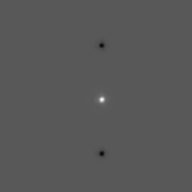
a)

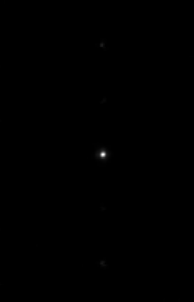
b)

Figure 1: a) Chopped and nodded image of the bright star BS 1370; the black circles are the negative counterparts of the star, generated by the chopping and nodding technique. b) The restoration of image a) obtained by means of our method, using the second stopping rule based on the average relative discrepancy; the negative counterparts have been completely removed (linear-scale representation).

Figure 1a) shows an image of the bright star BS 1370 obtained at UKIRT on 1996 August 26-27 through a broad-N band filter ($\lambda_{eff}=10.16\mu$m, $\Delta\lambda=5.20\mu$m). The integration times were set to 6.1 milliseconds/frame and 12 seconds total, chopping at $\approx 2$Hz with $\Delta=10$ arcseconds throw in the N-S direction ( $K=36$ ). Image post-processing consisted in filtering out some electronic noise in 1 out of 16 preamplifier channels and a counterclockwise rotation by $\simeq 2.3^{\circ}$. After post-processing the standard deviation of the noise is estimated using 10 columns in the blank region of the image. The value we obtain is $\sigma\simeq 10.6$ counts/pixel and this is the value to be used when applying the stopping rule based on equation (13). The corresponding value of $\varepsilon$ to be used according to equation (14), is about $0.033$. Note that the maximum value of the star intensity is $2.\ 10^{4}$ counts. Since the restoration method reduces this value by a factor of about 2 (see equation (5)), it should also reduce the noise by a similar factor. In the following we denote by $\sigma_{r}^{2}$ the variance of the noise in the restored image. It is estimated on the same columns used for the estimation of $\sigma^{2}$.

We have applied the method to the image of Figure 1a), using the two stopping rules introduced in Section 2. Using the first one, the algorithm performs only one iteration when the column does not contain signal; the maximum number of iterations is $44$ in the case of the column through the maximum of the star. After restoration, the peak value becomes $1.04\ 10^{4}$ and the variance of the noise is $\sigma_{r}\simeq 1.7$ counts/pixel. Therefore noise is reduced by a factor $6$. This very high noise reduction is due to the strong smoothing effect of the first iterations of the Landweber method. As a consequence the high frequency components of the noise are supressed. Regarding photometric accuracy the integrated flux (estimated through standard multi-aperture photometry) equal to $1.03$ the flux of the original image, i.e. photometric accuracy is preserved within $3\%$.

Using the second stopping rule, with $\varepsilon=0.033$, the algorithm stops after $13$ iterations. The $\sigma_{r}$ is smaller than $\sigma$ by a factor $2.5$ while photometric accuracy is now preserved within $0.4\%$. We emphasize that the noise reduction we obtain is just what we expect because, as already pointed out above, the restoration algorithm reduces the signal by a factor of 2.

This example clearly illustrates that the method assures noise reduction and rather good photometric accuracy. Both effects depend on the number of iterations and, using our two stopping rules, it results that the first one provides an excessive noise reduction and a poorer photometric accuracy with respect the second one. For these reasons the second stopping rule seems to be preferable.

Concerning artifacts, the two deep negatives counter-images created by the chopping and nodding technique are completely removed. Since the linear scale used in Figure 1b) makes difficult to notice the presence of any type of problem we plot in Figure 2 the profiles of the original and restored image along the column passing through the star maximum. The profile of the original image has been divided by 2 for comparison and the range of the ordinates reduced to $\pm 10\%$ the stellar maximum. It can be seen that the stellar profile is reproduced with great accuracy and that the two large negative counterparts of the original image are replaced by two small positive ghosts, similar to spikes. The integrated photometry of these spikes is about $3.5\%$ the stellar flux of the restored image. Besides these spikes two other positive ghosts appear at distances $\pm 2\Delta$, outside the original target. Their integrated fluxes are about $10\%$ the stellar flux. We point out again that the positions of these ghosts can be exactly predicted since they are located at distances which are multiple of the chopping throw.

According to our stopping rules, changing the value of $\varepsilon$ will also change the number of iterations: more precisely decreasing $\varepsilon$ increases $k$. The comparison of the results obtained with different number of iterations allows us to provide the following rule of thumb: an increase of iterations will cause the noise of the restored image to increase, as well as the integrated flux of the star. This is first underestimated and then overestimated by the algorithm.

3.3 Faint point sources

In order to test the method near the sensitivity limit, we apply our algorithm to an image containing two faint and isolated point sources, the system DH/DI Tau (Meyer et al. (1997)). The observational parameters and post-processing are similar to those presented in Section 4.2, with a total integration time $t_{int}=250$ s. Again, since the chopping direction was not perfectly aligned to the array columns, the image has been properly rotated before applying the inversion algorithm.

In our analysis we have considered only the central part of the original image (more precisely the columns from $26$ to $106$) in order to eliminate the incomplete lateral columns present in the rotated image, which could prevent an accurate estimate of $\varepsilon$. After rotation $\sigma$ is about $4$ counts/pixel and the corresponding value of $\varepsilon$ is about $.5$. This large value of $\varepsilon$ implies that we have an example of a very noisy image.

We have used again the two stopping rules of Section 2 with these values of $\sigma$ and $\varepsilon$. The number of iterations allowed by the two criteria is now very small (in the case of the second one, just one iteration). The first criterion provides $\sigma_{r}=0.6$ and underestimates the integrated fluxes of DH Tau (the bright source) and DI Tau by about $20$%. The second criterion provides again $\sigma_{r}=0.6$ and underestimates the integrated flux of DH Tau by about $15$% while correctly reproduces that of DI Tau. Therefore both criteria provide a considerable noise reduction but the second criterion works better even if the integrated flux of the brighter star is not really satisfactory.

This result is due to the property of the discrepancy principle discussed in Section 2. For this reason we reapplied the algorithm by stopping the iterations when $\varepsilon_{j}^{(k)}\leq\sigma/2=2$, in the case of equation (13), and when $\varepsilon^{(k)}\leq\varepsilon/2=2.5$, in the case of equation (14). In this case, the first method provides $\sigma_{r}=1$ and the integrated flux of DH Tau is underestimated by $5$% while that of DI Tau is overestimated by $5$%. The second criterion provides $\sigma_{r}=1.2$ and an underestimation of about $3.5$% for DH Tau and of $0.7$% for DI Tau. Again the criterion based on the average relative discrepancy turns out to provide better results, since both integrated fluxes are in nice agreement with the flux measured before the inversion.

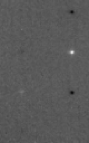
a)

b)

Figure 3: a) Original image of the system DH/DI Tau (80 columns). b) Restored image obtained using the second stopping rule of Section 2 with $\varepsilon=0.25$ (linear-scale representation).

The original image (after rotation) as well as the best restored image are displayed in Figure 3. In the original image DH Tau is the brighter source, clearly visible with its two negative counterparts, while DI Tau is the fainter source $\approx 15$ arcseconds to the S-W. The derived fluxes, as reported by Meyer et al. (1997), are $F_{N}=0.137\pm 0.005$Jy (6.26 mag) for DH Tau and $F_{N}=0.030\pm 0.005$Jy (7.90 mag) for DI Tau. The restored image shows no spikes or ghosts so that the negative counterparts of the brightest star (DH Tau) appear properly cancelled.

It must be noted that the rotation introduces a certain amount of high-frequency noise filtering depending on the rotation angle and origin. To investigate the noise decrease independently of the particular rotation/filtering applied, we added, somewhat arbitrarily, that amount of uniform Gaussian noise needed to preserve the average noise level of the original (before rotation) image. This new image has $\sigma\simeq 7$ counts/pixel and $\varepsilon\simeq 0.6$. By applying the method with the stopping based on the average relative discrepancy (using a reduction of $\varepsilon$ by a factor of 2) we obtain a result very close to the previous one still with a correct noise reduction and a non-significant marginal variation of photometric accuracy.

From the analysis of the restoration of isolated sources, we conclude that the criterion based on the average relative discrepancy provides better results. Moreover, in the case of very noisy images, it is convenient to reduce by a factor $2$ the value of $\varepsilon$ obtained from the $\sigma$ of the noise. We will adopt these rules in the following sections.

3.4 Bright extended sources

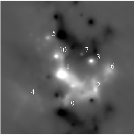
Figure 4: Raw N-band image of the Galactic Center with 10″chopping throw. The compact sources are labeled according to Becklin et al. (1978). The extended black regions are negative counterparts of the extended bright sources.

In this subsection we show how the algorithm performs when bright point sources coexist with fainter extended structures, i.e. when the field is characterized by high dynamic range signal. The central parsec of the Galaxy represents an ideal target in this respect, also because most of its prominent features lie within the MAX’s field of view. The image presented here (Figure 4) has been obtained on the night of 11 April 1998 on UKIRT with adaptive tip-tilt correction. We used a “N-narrow” filter with $\lambda_{c}=11.6~{}\mu$m, $\Delta\lambda=2.5~{}\mu$m, chopping throw $\approx 10"$ in the north-south direction, and 119.6 seconds total integration time on source (i.e. on the positive image). The airmass was $z=1.55$.

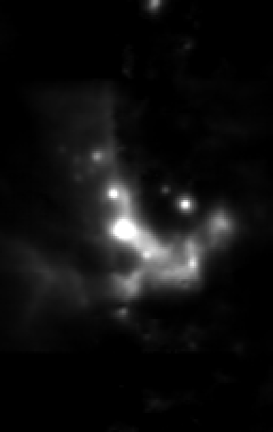
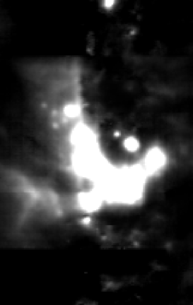
Figure 5: Restored images of the Galactic Center. The two pictures are obtained with two different cuts in the gray scale to evidence the full dynamic range of the image.

Once again, before applying the inversion algorithm, we had care of rotating the image by 0.7 degrees clockwise in order to align the chopping direction to the array columns. The image was also expanded to a $256\times 256$ size, in order to get a chopping throw $\approx 74.9$ pixels, allowing us to run the algorithm with $K=75$. Due to the complex structure of the source, almost entirely filling the field, we were unable to get a meaningful estimate of $\sigma$ using a sufficiently broad black part of the image. Given the brightness of the source, we have applied the criterion based on the average relative discrepancy assuming $\varepsilon=0.08$. The algorithm stops after 63 iterations. In Figure 5 we present the reconstruction result with two different cuts, in order to evidence the full dynamic range of the image.

The reconstructed image clearly shows several details, both of the “northern arm” and of the “bar”, which were barely visible or completely lost in the negative features of the original image. Quite remarkably, the algorithm correctly finds the IRS 8 source at the very last rows (top) of the reconstructed image. Moreover photometry of sources like IRS 7 turns out to be more reliable once the local patchy negative background has been removed.

On the other hand, the reconstructed image is not entirely free from Type A) artifacts. Ghosts of the brightest sources are clearly visible in the lower and upper part of the image. Especially IRS 1 produces a bright artificial spot $\approx 5"$ south of IRS 9, but virtually every bright IRS source generates some signature at the position of his negative counterparts, and in some case even at the corresponding multiple distances. To illustrate more in detail how artifacts look like, we plot in Figure 6 the vertical cut passing through IRS 1 on both the original and reconstructed image. The original image (thin line) shows the two negative “valleys” at pixels yr. 20 and yr. 94. At the same places, the reconstructed image presents two residual peaks, and especially at pixel yr. 20 the ghost feature appears prominent.

Methods for the reduction of these artifacts will be proposed in the next Section.

3.5 Faint extended sources

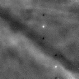
a)

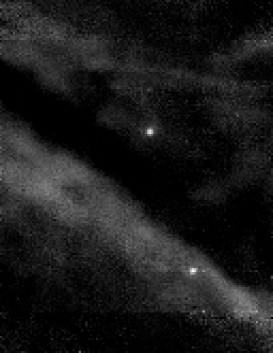
b)

Figure 7: a) Raw image of the Orion bar with 5″chopping throw. b) The restored image obtained after $49$ iterations ($\varepsilon=0.1$) (linear-scale representation).

Here we apply the algorithm to the case of diffuse emission completely filling the field. It is clear that, in this situation, no algorithm can reconstruct the absolute value of the original image, lost due to the differential observing technique. In Figure 7a) we present the image of an area within the Orion nebula taken at UKIRT on the night of the 9th February 1997 through the standard N-band filter. The main observing parameters were: integration time 10 ms/frame and 491.52 s total on source, chopping throw $\approx 5$ arcseconds in N-S direction, airmass $z\simeq 1.23$.

The field is located approximately 2 arcminutes S-E of the Trapezium stars and contains two point sources. That on top is the proplyd HST8=206-446 (O’Dell et al. (1993), O’Dell & Wong (1996)). The diffuse diagonal feature crossing the field is the Orion “bar”, i.e. the ionization front created by the Lyman-C photons produced by the Trapezium stars, $\theta^{1}C$ in particular.

An estimate of the noise has been attempted by analysing regions of the original image characterized by a rather uniform intensity distribution. We have obtained $\sigma\simeq 4000$ counts/pixel and the corresponding value of $\varepsilon$ is $0.2$. Therefore we have another example of a rather noisy image. For this reason we have used the second stopping rule with $\varepsilon=0.1$. The corresponding number of iterations turns out to be $49$.

The result of the reconstruction, performed on the original image without any rotation/filtering, is presented in Figure 7b). It can be seen that the restored image results nicely free from Type A) artifacts: both stellar images appear properly reconstructed with no relevant ghosts. The bar structure turns out to be more detailed, but the effect of its negative counterpart on the northern side is a flat reconstruction with a large number of zeros. This is a typical example of a Type B) artifact better evidenced in Figure 8 where we plot vertical cuts through the HST8 maximum both in the original image and in two restored images obtained with $\varepsilon=0.2$ and $\varepsilon=0.1$ respectively. The Type B) artifact corresponding to the large negative counterpart of the “bar” looks the same in the two restorations. Their comparison allows us to conclude that an increase in the number of iterations enhances both the star peak and the “bar”. Again the noise is reduced by the restoration algorithm.

3.6 Bright sources outside the field

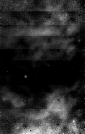
b)

Figure 9: a) Raw image of the Orion nebula, centered on proplyd 167-231, with 10″chopping throw. b) The restored image with discrepancy $0.02$ (linear-scale representation).

Before concluding this section, we must refer to that kind of artifacts that often arise when the image to be restored contains the negative counterpart of bright extended sources lying outside the field. At the end of Section 3 they were classified as Type C) artifacts. They appear as a series of horizontal jumps in the reconstructed images, with periodicity that depends on $K$ and $K_{1}$. As an example, we show in Figure 9a) an image of the Orion nebula centered on the dark-silhouette proplyd 167-231 (Robberto, Beckwith & Herbst (1999)) taken with similar parameters of Figure 7, except for the 10″chopping throw. The corresponding restored image, obtained with average relative discrepancy $\epsilon=0.02$, is displayed in Figure 9b) and clearly shows the horizontal jump artifacts. In the next Section we will describe a simple method for efficiently reduce this kind of artifacts.

4 Artifacts reduction

We propose three methods which can be used to eliminate the artifacts illustrated in the previous Section. The first is both observational and computational and it is a way for reducing Type A) and Type B) artifacts. The second is only computational since it is based on manipulations performed on a single chopped and nodded image and acts only on Type C) artifacts. The last one is again observational and computational and can be also used for reducing the Type C) artifacts.

4.1 Inversion of multiple images of the same object

The analysis of the previous Section indicates that the ghosts of a very bright source, i.e. Type A) artifacts, or the areas with zero value, i.e. Type B) artifacts, are very frequent and may reduce the quality of the restorations. As we observed in Section 2, these artifacts are due to a lack of information in the chopped and nodded image (the missing frequencies). Images containing different pieces of information can then be restored by means of the projected Landweber method and recombined. It is clear that no pair of values of $K$ should have a common divisor. In practice, this procedure is similar to that suggested by Beckers (Beckers (1994)), but is completely different in what concerns data processing. Note that this approach reduces all types of artifacts.

The most simple kind of recombination is to take the arithmetic mean of the various restored images over the common domain, coincident with the size of the restored image with the smallest value of $K$. This approach was applied to simulated images, finding that it allows to reduce significantly the restoration error (Bertero et al. (1999)).

If more than two images are available, we have verified that the median usually provides better results. If only two images are available, it seems more convenient to take the smallest value. In case of images containing only compact sources, this recombination removes completely the Type A) artifacts. In case of images containing both compact and extended sources, the bright ghosts over dark background are removed while the dark ghosts over bright background are preserved.

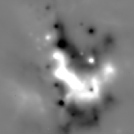
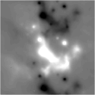
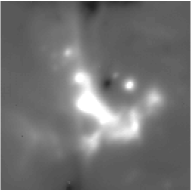
a)	b)	c)

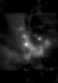
d)

e)

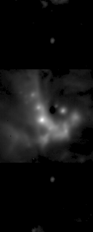
f)

Figure 10: Chopped and nodded images of the galactic center with: a) $7\arcsec$ chopping throw, $K=29$; b) $13\arcsec$ chopping throw, $K=51$; c) $25\arcsec$ chopping throw, $K=95$. d), e), f) are the restorations of a), b) , c) respectively (the restorations are represented using square root scale).

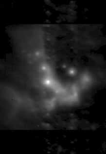
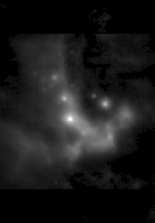
a)	b)

Figure 11: Recombined images of the Galactic Center, obtained taking: a) the arithmetic mean, b) the median of five restored images; three of them are shown in Figure  10) (square root scale representation).

In order to validate this approach, four other images of the Galactic Center (besides that one presented in Section 3.4) were taken in April 1998. The five images have $\approx 7\arcsec,10\arcsec,13\arcsec,17\arcsec,25\arcsec$ chopping throws, always in the N-S direction, corresponding to $K=29,38,51,67,95$. After the inversion, the size of the common region is $128\times 186$ pixel. Figure  10 shows the original images with $7\arcsec,13\arcsec,25\arcsec$ chopping throw, as well as the corresponding restored images. The ghosts of the brightest point source can be easily identified. In Figure  11 we show the combination of the 5 reconstructed images using the mean (a) and the median (b) of the stack. As we anticipated, the median image provides the better reconstruction, just marginally affected by Type A) artifacts. Figure  11 shows that only the restoration in the observation region is entirely reliable, whereas the restoration outside strongly depends on the chopping amplitude.

It is certainly possible to get better results by using more refined procedures for recombining the various restored images. In particular, one can observe that the position of the ghosts can be readily foreseen once the reconstructed image is available. For each image it is possible to build a map of the areas possibly affected by ghosts where other images should better be used, and therefore a weight function describing the relative reliability of the various images may be introduced. The investigation of this approach is in progress.

4.2 Multiple inversions from the same image

This is a useful method for reducing the Type C) artifacts, i.e. jumps in the brightness distribution of the restored images but it does not modify the Type A) and Type B) artifacts whenever they appear. It is directly suggested by the observation that the positions of the discontinuities are related to the values of $K_{1}$ and $K$. Since $K$ is fixed, the only way for changing these positions is to change $K_{1}$. This can be obtained by reducing the value of $N$, i.e. by removing a certain number of rows from the original chopped and nodded image.

Starting with a chopped and nodded image with columns of length $N$ and chopping amplitude $K$, by applying the inversion algorithm one obtains a restored image with columns of length $N+2K$ and jumps at the rows indicated at the end of Section 3. Removing $M$ rows both from the top and from the bottom of the original image a reduced image with columns of length $N-2M$ is produced. Let us assume $K_{1}>2M$, so that the value of $q$ does not change while $K_{1}$ is replaced by $K_{1}^{\prime}=K_{1}-2M$. By applying again the inversion method to the reduced image, one obtains a new restored image with columns of length $N+2K-2M$ and jumps at the rows $K_{1}^{\prime},K,K+K_{1}^{\prime},\cdots,K_{1}^{\prime}+(q+1)K,(q+2)K$. The pixels of one column of this image, with $n$ ranging from 1 to $N+2K-2M$, correspond to the pixels of the same column of the previously restored image with $n$ ranging from $M+1$ to $N+2K-M$, so that the jumps of the second restored image occur at the rows $K_{1}-M,K+M,K+K_{1}-M,\cdots,K_{1}+(q+1)K+M,(q+2)K-M$ of the first one. In other words, the effect produced by the reduction of the original image is a shift of length $M$ towards the top of the restored image, for the jumps of odd order and a shift of length $M$ towards the bottom, for the jumps of even order. If the positions of the jumps in the two restored images do not coincide, by taking the arithmetic mean of the two images over the common domain one obtains a reduction of the jumps by a factor of 2. The same result holds true also when $2M>K_{1}$, as it can be deduced by observing that, for the reduced image, $q$ is replaced by $q^{\prime}=q-1$ and $K_{1}$ by $K_{1}^{\prime}=K_{1}+K-2M$.

This procedure can be extended to the case where several reduced images are used in addition to the original one. If the total number of images is $p$ and if the rows are removed in such a way that all positions of the jumps in the various restored images are different, then, by taking the arithmetic mean of these images over the common domain (which coincides with that of the shortest restored image) we obtain a reduction of the jumps by a factor of $p$. The resulting average image will produce a much better result than that obtained by a single inversion.

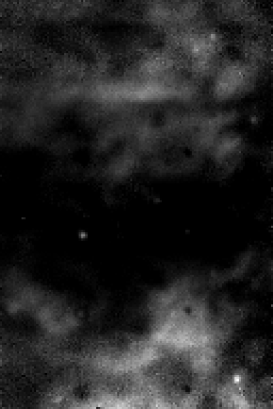
Figure 12: Reconstruction of the image of Figure  9a) obtained by means of the reduction and averaging procedure described in the text (linear-scale representation).

Figure 12 shows the result obtained by applying this procedure to the image presented in Figure 9a). The average image is the arithmetic mean of six restored images, one directly obtained from the original image and five obtained by removing respectively 1,2,3,4, and 5 rows from the top and the bottom of the original one. The jumps are considerably attenuated while the multiple ghosts of the bright stars remain unchanged.

4.3 Inversion of pasted images

The Type C) artifacts in the restored image do not appear or, at least, are very weak if no significant extended source exists outside the observation region. However, it is in general possible to take images of adjacent regions in order to build a mosaic encompassing the brightest sources of the region. If no significant extended source exists below and above the mosaic, the algorithm can be run on the combined image to obtain a better reconstruction.

We have tested this approach on a couple of images of the giant HII region W51. The observations were carried out with MAX on August 29-30 1997 through the broad N-band filter. The chopping frequency was 2.2 Hz and the chopping throw $\approx~{}30\arcsec$ in the N-S direction. The integration time was set to 10.2 ms per frame and 40 seconds total on source (Ligori, Robberto & Herbst (1999)).

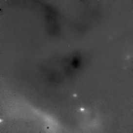
a)

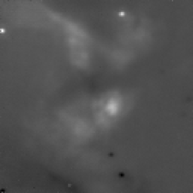
b)

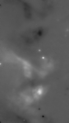
c)

Figure 13: The two original images of the W51-IRS 1 region and their mosaic: a) Original image of a region 29 arcseconds north of W51 IRS1. b) Original image of IRS1. c) Mosaic obtained by combining the two previous images.

The two images (Figure 13) are centered respectively on W51 IRS1 (Figure 13b)) and 29 arcseconds north of W51 IRS1 (Figure 13a)). Figure 13b) shows that, due to the large chopping throw, the bright star on top has a negative counterpart close to the bottom of the image. Another negative counterpart is visible nearby, $\approx 8\arcsec$ to the south of IRS 1. From this image alone there is no way to specify if this second source lies above or belove the field. Figure 13a) reveals that it lies above.

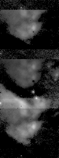
a)

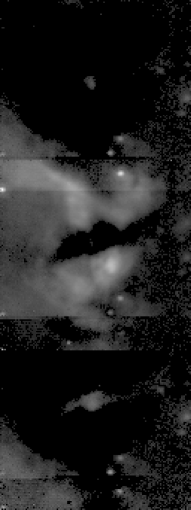
b)

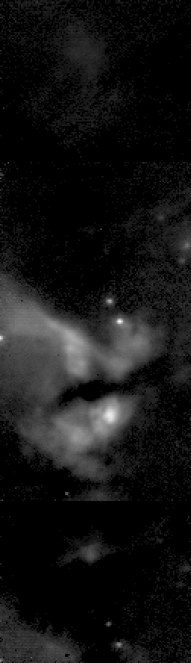
c)

Figure 14: Reconstruction of the three images of W51: a) Reconstruction of the image of Figure 13a). b)Reconstruction of the image of Figure 13b). c) Reconstruction of the mosaic of Figure 13c) (square root scale representation).

The reconstruction of these two images produces the results displayed in Figure 14a) and Figure 14b) respectively. These results are clearly unacceptable. On the other hand, the two images can be combined to form a $128\times 224$ pixel mosaic (Figure 13c)). Figure 14c) shows the corresponding reconstruction with dynamic range emphasizing the lowest counts. With respect to Figure  14a,b), the improvement in image is striking: the horizontal discontinuities within the central field have disappeared, and also the other artifacts are significantly reduced. Only discontinuities at the border of the observation region defined by the mosaic are still visible. Note that the “hole” present between IRS1 and the north rim is real, as near-IR data clearly indicate the presence of a dark ridge North of IRS1. Note also the source $\approx 25\arcsec$ to the south of IRS 1, visible in the 20 $\mu$m map of Genzel et al. (1982) and correctly reconstructed by our algorithm.

5 Comments and Conclusions

We have considered the problem of the reconstruction of astronomical data taken at mid-IR wavelengths in chopping and nodding mode. Studying the mathematical properties of the corresponding under-determined linear system, we have proposed an iterative method for approximating the positive solution of minimal r.m.s. value. We have implemented the algorithm and tested it on astronomical data taken in various observing runs at the UKIRT telescope with the MAX camera. We have investigated the nature of the artifacts affecting the restored images and suggested various computational and observational strategies for their reduction. We find that if an extended source is observed with a few different chopping throws, possibly building a mosaics if the source extends beyond the detector field of view, our algorithm can provide a reliable reconstruction of the source brightness.

We finally remark that on the basis of the MAX experience the proper setup of the camera at the telescope is crucial to get the best results from our reconstruction method. It can be useful in this respect to provide our check-list for the setup of MAX on UKIRT.

Assuming that the chopping-nodding direction has been chosen to be N-S:

1. Select chopping throws close to a common multiple of the instrument pixel size and of the guide/tip-tilt camera pixel size. Use preferably chopping throws larger than 1/6 the array size for best reconstruction (see BBDR99).

2. Align the chopping direction to the detector orientation: point to a bright star at the edge of the field, and make sure that for large chopping throws $x$ coordinates of the positive and negative centroids are as close as possible within the same column. The chopping direction will be in general different from the real N-S direction.

3. Align the nodding direction to the chopping direction. If the telescope software implements the nodding as a simple jump of the telescope to an “offset” position, be sure that both the right ascension and declination (or amplitude and position angle) of the offset beam have been given. Note that both values will change with the chopping throw.

4. If the guide camera/cross-head moves when the telescope is pointed to the offset beam, make sure that also for the camera offset both right ascension and declination have been introduced.

There is a last point that deserves some attention as a potential limit to the accuracy of the method: field distortion. Off-axis reflectors are a preferred choice for mid-IR imagers, as they allow a compact and achromatic optical design. However, these systems are in general strongly affected by field distortion. Optical designers often trade field distortion for the ultimate optical quality. For thermal-IR work, it must be kept in mind that is still very difficult to obtain a good astrometric calibration, given also the scarcity of good calibration fields in this wavelengths regime.

Our code is free and is available on request to the authors. Two versions are available, in C and in IDL. For the IDL version, the typical execution time for the inversion of a $128\times 128$ image is of the order of a few tens of seconds on a Ultra 10 SPARC station.

6 Acknowledgements

This work was partially funded by the Italian CNAA (Consorzio Nazionale per l’Astronomia e l’Astrofisica) under the contract nr. 16/97.

The authors are indebted to S.Ligori for providing the W51 images in advance of publication. M.R. acknowledges Steven Beckwith and Tom Herbst for discussions on this subject during the long nights spent observing on UKIRT.

Figure 2: a) Vertical cuts passing through the maximum of BS 1370 : original image (full line), reconstructed image (dotted line). For comparison, the profile of the original image has been divided by 2.

Figure 6: Vertical cuts through the IRS 1 source in the original image (thin line) and in the reconstructed image (thick line). Pixel 0 is at the bottom of the image.

Figure 8: Vertical cuts passing through the HST8 maximum for the original image (dotted line), the restored image with $\varepsilon=0.2$ (dashed line), obtained after $9$ iterations, and the restored image with $\varepsilon=0.1$ (full line), obtained after $49$ iterations.

a)

References

- Beckers (1994) Beckers, J. M. 1994, Proc. SPIE, 2198, 1432
- Becklin et al. (1978) Becklin, E. E., Matthews, K., Neugebauer, G., & Willner S. P. 1978, ApJ, 219, 121
- Bertero & Boccacci (1998) Bertero, M., & Boccacci, P. 1998 Introduction to Inverse Problems in Imaging, (Bristol: IOP Publishing)
- Bertero et al. (1998) Bertero, M., Boccacci, P. & Robberto, M. 1998, Proc. SPIE, 3354, 877 (BBR98)
- Bertero et al. (1999) Bertero, M., Boccacci, P., Di Benedetto, F., & Robberto, M. 1999, Inverse Problems 15, 345 (BBDR99)
- Eicke (1992) Eicke, B. 1992, Num. Funct. anal. Opt. 13, 413
- Genzel et al. (1982) Genzel R., Becklin E. E., Wynn-Williams C. G., Moran J. M., Reid, M. J., Jaffe D. T., & Downes D. 1982, ApJ, 255, 527
- Kaeufl (1995) Kaeufl, H. V. 1995, in ESO Conference and Workshop Proc. 53, Calibrating and Understanding HST and ESO Instruments, ed. P. Benvenuti, (Garking, Germany), 159
- Kaeufl et al. (1991) Kaeufl, H. U., Bouchet, P., Van Dijsseldonk, A., Weilenmann, U. 1991, Experimental Astronomy 2, 115
- Ligori, Robberto & Herbst (1999) Ligori, S., Robberto, M., Herbst, T. M. 1999, A&A, in preparation
- Meyer et al. (1997) Meyer M. R., Beckwith, S. V. W., Herbst, T. M., & Robberto M. 1997, ApJ, 489, L173
- O’Dell et al. (1993) O’Dell, C. R., Wen, Z., & Hu, X. 1993, ApJ, 410, 696
- O’Dell & Wong (1996) O’Dell, C. R., & Wong, K. 1996, AJ, 111, 846
- Robberto, Beckwith & Herbst (1999) Robberto, M., Beckwith, S. V. W., & Herbst, T. M. 1999, in preparation
- Robberto & Herbst (1998) Robberto, M. & Herbst T. M., 1998, Proc. SPIE, 3354, p.711
- Thomas & Duncan (1993) Thomas, M. E., & Duncan, D. D. 1993, in The Infrared and Electro-Optical Systems Handbook, Vol. 2, Atmospheric Propagation of Radiation, ed., F. G. Smith, (Environmental Information Analysis Center, Ann Arbor, MI, and SPIE Optical Engineering Press, Bellingham, WA), 3