First results of UVES at VLT: abundances in the Sgr dSph

Abstract

Two giants of the Sagittarius dwarf spheroidal have been observed with the UVES spectrograph on the ESO 8.2m Kueyen telescope, during the commissioning of the instrument. Sgr 139 has [Fe/H]$=-0.28$ and Sgr 143 [Fe/H]$=-0.21$, these values are considerably higher than photometric estimates of the metallicity of the main population of Sgr. We derived abundances for O, Na, Mg, Al, Si, Ca, Sc, Ti, V, Cr, Mn, Co, Ni, Cu, Y, Ba, La, Ce, Nd and Eu; the abundance ratios found are essentially solar with a few exceptions: Na shows a strong overdeficiency, the heavy elements Ba to Eu, are overabundant, while Y is underabundat. The high metallicity derived implies that the Sgr galaxy has experienced a high level of chemical processing. The stars had been selected to be representative of the two main stellar populations of Sagittarius, however, contrary to what expected from the photometry, the two stars show a very similar chemical composition. We argue that the most likely explanation for the difference in the photometry of the two stars is a different distance, Sgr 143 being about 2Kpc nearer than Sgr 139. This result suggests that the interpretation of colour – magnitude diagrams of Sgr is more complex than previously thought and the effect of the line of sight depth should not be neglected. It also shows that spectroscopic abundances are required for a correct interpretation of Sgr populations.

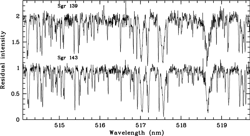
Figure 1: The spectra of the two stars in the region of the Mg I b triplet. The spectrum of Sgr 139 has been shifted vertically by one unit for display purposes. Wavelengths are observed wavelengths, not shifted to rest.

1 Introduction

In the recent years our ideas on galaxy formation and evolution have considerably developed, and it is generally acknowledged that it is a complex process which may well take different paths in different galaxies. Much attention is being devoted to dwarf spheroidal galaxies, essentially for two reasons: 1) they seem to be relatively simple systems, typically characterized by a single stellar population; in such a system we hope to be able to isolate some of the key ingredients of the phenomenon; 2) Interaction of these dwarf galaxies with large galaxies (such as our own or the Andromeda galaxy) could, in principle, play an important role in shaping the morphology of the large galaxies. The nearest members of the class, the dwarf spheroidals of the Local Group, are close enough that their stars are amenable to detailed analysis with the same techniques employed to study Galactic stars, with the advent of the new 8m class telescopes. In this paper we report on such an observation: the first detailed chemical analysis of two stars in the Sgr dwarf spheroidal based on high resolution spectra obtained with the UVES spectrograph on the ESO 8.2m Kueyen telescope. Ever since the discovery of Sgr (Ibata et al 1994) photometric studies have shown the red giant branch (RGB) of Sgr to be wider than expected for a population with a single age and metallicity. This has been generally interpreted as evidence that Sgr displays a spread in metallicity which is likely due to different bursts of star formation. Ibata et al (1995) found a mean metallicity of [Fe/H]=-1.25 and their metallicity distribution displays a spread of over 1 dex. Sarajedini & Layden (1995) found a main population with [Fe/H]= -0.52 and suggested the possible existence of a population of [Fe/H]$\approx-1.3$. Mateo et al (1995) provide a mean metallicity of $-1.1\pm 0.3$, Ibata et al (1997) estimate metallicities in the range $-1.0-0.8$, Marconi et al (1998) $-1.58-0.7$ , Bellazzini et al (1999) $-2.1,-0.7$. The age of Sgr may not be disentangled from its metallicity, from Main Sequence fitting, Fahlman et al (1996) found acceptable solutions for an age of 10 Gyr and metallicity $-0.8$ or an age of 14 Gyr and a metallicity $-1.3$. Clearly if Sgr may not be described as a single population the concepts of age and metallicity loose some of their significance; Bellazzini et al (1999) proposed an extreme scenario in which star formation began rather early and continued for a period longer than 4 Gyr. Foreseeing the potentiality of UVES to perform detailed abundance analysis of these stars, to confirm or refute the photometrically inferred spread in metallicity, we undertook already in 1995 observations of low resolution spectra of photometrically identified (Marconi et al 1998) Sgr candidates. The main purpose was to obtain confirmed radial velocity members of Sgr for subsequent high resolution follow-up with UVES. From the low resolution spectra we also devised a method to obtain crude metallicity estimates from spectral indices defined in the Mg I b triplet region. The two stars were selected from this low-resolution study of Sgr with photometry and abundance estimates which suggested these stars to differ by at least 0.5 dex in metallicity.

Table 1: Basic Data

#	$\alpha_{2000}$	$\delta_{2000}$	$V$	$(V-I)_{0}$	$T_{eff}$	log g	$\xi$
					K		kms-1
139	18 53 50	$-30$ 30 45	18.33	0.965	4902	2.5	1.4
143	18 53 49	$-30$ 31 60	18.15	0.947	4932	2.5	1.5

Table 2: Mean abundances

	[X/H]	$\sigma$	n	[X/H]	$\sigma$	n
	139			143
O I	$<-0.53$	–	1	$-0.37$		1
Na I	$-0.61$	0.12	2	$-0.78$	0.17	3
Mg I	$-0.33$	0.11	2	$-0.44$	0.12	3
Al I	$-0.52$	0.08	3	$-0.40$	0.26	3
Si I	$-0.35$	0.26	5	$-0.28$	0.09	5
Ca I	$-0.49$	0.12	5	$-0.47$	0.21	4
Sc II	$-0.67$	0.05	2	$-0.67$	0.20	2
Ti I	$-0.19$	0.13	7	$-0.37$	0.14	7
Ti II	$-0.31$	0.07	2	$-0.46$	0.06	2
V I	$-0.21$	0.16	2	$-0.44$	0.05	2
Cr II	$-0.32$		1	$-0.35$		1
Mn I	$-0.41$		1	$-0.30$		1
Fe I	$-0.28$	0.16	15	$-0.21$	0.19	15
Fe II	$-0.33$	0.14	3	$-0.23$	0.04	4
Co I	$-0.34$	0.21	2	–	–	–
Ni I	$-0.56$	0.16	6	$-0.44$	0.21	6
Cu I	$-0.45$		1	$-0.22$		1
Y II	$-0.61$	0.08	3	$-0.66$	0.13	4
Ba II	$-0.08$		1	$-0.10$		1
La II	$+0.30$	0.30	3	$+0.33$	0.23	3
Ce II	$+0.15$	0.06	3	$+0.00$	0.13	3
Nd II	$+0.12$	0.27	5	$+0.09$	0.19	8
Eu II	$+0.05$		1	$+0.05$		1

Table 3: Line data and abundances for Fe

Ion	$\lambda$	log gf	EW(pm)	$\epsilon$	EW(pm)	$\epsilon$
	nm		139		143
Fe I	585.5091	-1.76	4.12	7.56	4.24	7.61
Fe I	585.6083	-1.64	3.85	7.04	6.24	7.51
Fe I	585.8779	-2.26	1.97	7.14	2.37	7.27
Fe I	586.1107	-2.45	1.81	7.35	1.22	7.18
Fe I	506.7151	-0.97	7.46	7.06	8.34	7.24
Fe I	510.4436	-1.69	5.89	7.27	6.58	7.65
Fe I	510.9650	-0.98	–	–	7.90	7.24
Fe I	489.2871	-1.29	7.09	7.32	5.91	7.06
Fe I	552.5539	-1.33	6.25	7.13	-	–
Fe I	587.7794	-2.23	2.74	7.25	3.34	7.25
Fe I	588.3813	-1.36	7.88	7.18	9.15	7.43
Fe I	615.1617	-3.30	9.59	7.28	8.02	6.98
Fe I	616.5361	-1.55	5.98	7.17	6.46	7.26
Fe I	618.7987	-1.72	7.36	7.37	6.34	7.17
Fe I	649.6469	-0.57	6.26	6.97	8.45	7.38
Fe I	670.3568	-3.16	7.72	7.42	7.16	7.33
Fe II	483.3197	-4.78	2.72	7.34	1.94	7.27
Fe II	499.3358	-3.65	5.97	7.10	6.37	7.30
Fe II	513.2669	-4.18	–	–	3.98	7.33
Fe II	526.4812	-3.19	6.00	7.11	6.09	7.24

2 Observations and data reduction

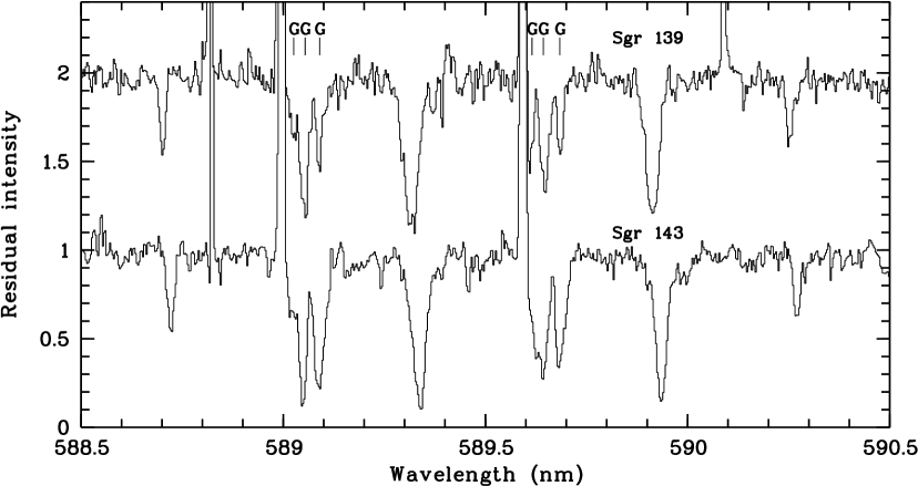
Figure 2: The spectra of the two stars in the region of the Na I D doublet. The spectrum of Sgr 139 has been shifted vertically by one unit for display purposes. Wavelengths are observed wavelengths, not shifted to rest. The absorptions due to Galactic interstellar gas are clearly visible and are marked with the label G.

The data were obtained during the Commissioning of UVES and have been released by ESO for public use. The spectra of the two stars, whose basic data is given in Table 1, were taken on the nights 2,3,4 and 6 October 1999. The slit was $1^{\prime\prime}$, which provided a resolution of $\sim 43000$ at 565 nm. We used only the red arm of UVES with the standard setting with central wavelength at 580 nm, which provides spectral coverage from 480 nm to 680 nm The detector was the mosaic of two CCDs composed of a EEV CCD-44 for the bluemost part of the echellogramme and an MIT CCID-20 for the redmost part. Both CCDs are composed of $4096\times 2048$ square pixels of 15 $\mu m$ side. We used a $2\times 2$ on–chip binning, without any loss of resolution, given the relatively wide slit used. For each of the two stars three one-hour exposures were collected, under median seeing conditions, allowing to reach a signal to noise ratio of $\sim 30$ at 510 nm, confirming the excellent performance of the instrument (D’Odorico et al, 2000).

The data was reduced using the ECHELLE context of MIDAS; reduction included background subtraction, cosmic ray filtering, flat fielding, extraction, wavelength calibration and order merging. Each of the CCDs of the mosaic was reduced independently. The r.m.s. of the calibration was typically of the order of 0.2 pm for each order and in all cases less than 0.3 pm. Flat-fielding was highly successful and the single echelle orders were rectified to within $\sim 5$% by this process, except in the vicinity of CCD defects, where the correction was not always satisfactory. The three spectra available for each star were coadded without any shift in wavelength. By cross-correlation we estimated the shift between any pair of spectra to be less than 0.5 pixel, so we decided not to perform any shift. This results in a very slight degradation of the resolution, which is not an issue for our analysis. The differences in barycentric correction were at most of 0.1 kms^-1, so no appreciable shift was expected from this cause either. The normalized and merged spectra were plotted superimposed on preliminary synthetic spectra for the purpose of line identification. A single velocity shift was adequate for all the spectra, confirming that the internal accuracy of our wavelength scale is better than 0.2 km/s. Portions of the normalized spectra of the two stars are displayed in figures 1 and 2.

3 Analysis

Our analysis is standard and essentially based on LTE model atmospheres. For each star we estimated effective temperature from $(V-I)_{0}$ through the colour–T_eff calibration for giants of Alonso et al (1999). We adopted log g = 2.5 for both stars, this value is compatible with the position of the stars in the colour–magnitude diagram, whichever the isochrone set considered. Furthermore we verified a posteriori that this gravity nearly satisfied the ionization equilibrium of both Fe I/Fe II and Ti I/Ti II . The atmospheric parameters are summarized in Table 1. The mean abundances for all the elements are given in Table 2.

With these parameters we computed model atmospheres using the ATLAS9 code (Kurucz 1993) using opacity distribution functions with microturbulence of 2 km/s and suitable metallicity.

We began by deriving the Fe abundance for both stars. We picked a set of lines which our preliminary synthetic spectra predicted to be substantially unblended, which had accurate laboratory or theoretical gf values and which spanned a range of line strengths. We excluded from the analysis lines stronger than $\log(EW/\lambda)=-4.8$ to avoid an excessive dependence on microturbulence and lines weaker than $\log(EW/\lambda)=-6.1$ to avoid lines which are too noisy.

For these lines we measured equivalent widths by fitting a gaussian with the iraf task splot and used these and the model atmosphere as input to the WIDTH9 code (Kurucz 1993). Some of the lines were removed from the analysis because they provided highly discrepant abundances. The microturbulence was determined by imposing that strong lines and weak lines give the same abundance. The results are given in Table 3. The excitation equilibrium for Fe I is very nearly satisfied for both stars (slopes are -0.05 dex/eV for star 139 0.13 dex/eV for star 143), we did not adopt an excitation temperature, so that the equilibria are better satisfied, since our lines cover a range of only about 2.7 eV, this means, that in the worst case (star 143) the slope predicts a difference of slightly over 0.3 dex between the highest and lowest excitation lines, this is $\sim 2\times$r.m.s.

As a check of our metallicity we derived Fe abundances also using MARCS models computed by Plez et al (1992). The difference is not significative: for both stars the MARCS models provide an Fe I abundance which is 0.02 dex larger than that provided by the ATLAS models, while for Fe II it is 0.07 dex larger for star 139 and 0.05 dex larger for star 143.

Having fixed the metallicity and the microturbulence we proceeded to determine all the other abundances with the same method, again we disregarded the too strong and too weak lines, with a few exceptions, such as Sc, Cu and Ba, for which only one or two lines were available, in order to get information on as many elements as possible. The line data and abundances are given in Table 4. In addition for some blended lines we resorted to spectrum synthesis using the same model-atmosphere and the SYNTHE code (Kurucz 1993). We did not take into account hyperfine splitting (HFS) for Sc, V, Mn, Co and Cu, however given that the abundances of these elements are coherent with those of other elements we do not expect corrections due to HFS to be very large. For Eu we determined the abundance from the Eu II 664.5 nm line, taking into account HFS splitting, the relevant data is given in Table 5. The error on the Eu abundances estimated from the quality of the fit is 0.15 dex.

The main result of this analysis confirms the impression gathered by a direct comparison of the spectra of the two stars: the stars are very nearly identical, the few differences in their spectra are quite likely determined by slightly different T_eff and log g, but not by chemical composition.

From the measure of the line centers of the unblendend lines used for abundances we determined the radial velocity for the two stars. We obtain the following heliocentric radial velocities $133.8\pm 0.8$ kms^-1 from 60 lines for star 139 and $143.8\pm 0.8$ kms^-1 from 57 lines for star 143, the quoted error is just the r.m.s. The measurement of the position of the atmospheric Na I D emission lines allowed to estimate the zero point shift to be less than 0.1 kms^-1, this, coupled with the excellent reproducibility of the wavelength scale from night to night induced us to assume a null zero–point shift. These heliocentric radial velocities support membership to Sagittarius, Ibata et al (1995) give a mean heliocentric radial velocity for Sgr of $140\pm 2$ kms^-1 and Ibata et al (1997) find the intrinsic velocity dispersion to be $11.4\pm 0.7$ kms^-1 and constant across the face of the galaxy. The N–body model of Sgr computed by Helmi & White (2000) displays a similar velocity dispersion, if only the stars with 100 kms${}^{-1}\leq v_{hel}\leq 180$ kms^-1 are included, as done by Ibata et al. However if this condition is relaxed the velocity dispersion turns out to be much larger, due to the contribution of stars in the debris streams. Given the above considerations it is not surprising that we find a difference of 10 kms^-1 between our stars. Our measured radial velocities compare quite well with those measured from our EMMI low resolution spectra (147 kms^-1 for star 139 and 154 kms^-1 for star 143, both are accurate to $\pm 15$ kms^-1).

We cannot rule out the possibility that the stars studied here belong to the Bulge, rather than Sgr. If they were at a distance of 8.5 Kpc, rather than 25 Kpc their log g should be $\sim 0.5$ dex higher than what we assumed, but such a difference is within the errors of the analysis. However the radial velocity ought to be a very good discriminant. By looking at Figure 1 of Ibata et al (1995) we see that the distribution of radial velocity of Bulge stars in directions which do not intercept the Sgr dSph, show a vanishingly small number of stars at the radial velocity of Sgr. Also the chemical composition suggests that the two stars do not belong to the Bulge: in fact Bulge stars are expected, theoretically, to have [$\alpha$/Fe]$>0$, even at solar metallicities. Observationally the situation is not so clear, however our distinctly solar [$\alpha$/Fe] is a clue against Bulge membership.

4 Discussion.

The metallicity of the two stars examined here is higher than all previous photometric estimates. Although it is possible that we happened to select two members of the high–metallicity tail of Sgr, this position is hardly tenable, the event of finding two such stars in a 9 square arcmin field must be quite rare. It is more likely that Sgr actually possesses a population, perhaps the main population, this metal–rich. For our two stars the Schlegel et al (1998) maps provide $E(B-V)=0.14$. By comparison Marconi et al (1998) used E(B-V)=0.18. The fact that the actual reddening could be 0.04 less than this could explain why the metallicity we find is 0.3 dex higher than the highest metallicity estimated by Marconi et al.

Table 4: Line data and abundances

Ion	$\lambda$	log gf	EW(pm)	$\epsilon$	EW(pm)	$\epsilon$
	nm		139		143
O I	630.0304	-9.82	$<1.5$	$<8.33$	2.08	8.49
Na I	498.2814	-0.95	–	–	syn	5.44
Na I	615.4226	-1.56	3.73	5.80	3.32	5.74
Na I	616.0747	-1.26	4.48	5.63	3.42	5.46
Mg I	571.1088	-1.83	11.48	7.32	10.16	7.12
Mg I	631.8717	-1.98	4.00	7.17	3.19	7.03
Mg I	631.9237	-2.20	–	–	3.24	7.26
Al I	669.8673	-1.65	2.88	5.95	syn	6.27
Al I	669.6788	-1.42	syn	6.04	syn	6.17
Al I	669.6023	-1.35	syn	5.87	syn	5.77
Si I	577.2146	-1.75	6.67	7.48	4.82	7.16
Si I	594.8541	-1.23	7.12	7.00	8.84	7.28
Si I	614.2483	-1.48	2.36	7.05	4.34	7.40
Si I	614.5016	-1.43	4.99	7.47	3.79	7.24
Si I	615.5134	-0.77	5.80	6.95	7.87	7.27
Ca I	615.6023	-2.20	1.81	5.77	–	–
Ca I	616.1297	-1.02	7.99	5.89	9.20	6.00
Ca I	616.6439	-0.90	–	–	8.01	5.66
Ca I	645.5598	-1.35	6.37	5.81	7.85	6.07
Ca I	649.9650	-0.59	9.95	5.70	9.95	5.69
Ca I	650.8850	-2.11	3.28	6.01	—	–
Sc II	552.6790	0.13	9.94	2.53	10.91	2.65
Sc II	632.0851	-1.77	1.92	2.46	1.62	2.36
Ti I	488.5082	0.36	9.92	4.88	8.97	4.63
Ti I	497.7719	-0.92	syn	4.66	syn	4.80
Ti I	497.8222	-0.39	syn	4.76	syn	4.60
Ti I	498.9131	-0.22	syn	4.76	syn	4.44
Ti I	499.7098	-2.12	syn	5.05	syn	4.70
Ti I	586.6452	-0.84	10.14	4.91	8.41	4.57
Ti I	612.6217	-1.42	6.40	4.76	6.72	4.83
Ti II	498.1355	-3.16	syn	4.76	syn	4.60
Ti II	499.6367	-2.92	syn	4.66	syn	4.52
V II	573.7059	-0.74	–	–	3.28	3.57
V II	613.5361	-0.75	syn	3.68	syn	3.50
V II	615.0157	-1.78	syn	3.91	syn	3.60
Cr II	488.4607	-2.08	3.76	5.35	3.76	5.32
Mn I	511.7934	-1.14	3.72	4.98	4.24	5.09
Co I	553.0774	-2.06	5.76	4.73	–	–
Co I	533.1452	-1.96	4.10	4.43	–
Ni I	585.7746	-0.64	2.74	5.41	4.38	5.75
Ni I	612.8963	-3.33	5.60	5.75	5.86	5.81
Ni I	613.0130	-0.96	1.89	5.61	1.88	5.62
Ni I	617.5360	-0.53	5.74	5.81	4.93	5.64
Ni I	617.6807	-0.53	5.73	5.81	7.86	6.21
Ni I	617.7236	-3.50	3.69	5.75	3.95	5.82
Cu I	510.5537	-1.52	13.10	3.99	11.80	3.76
Y II	488.3684	0.07	5.84	0.95	9.37	1.67
Y II	498.2129	-1.29	3.35	1.71	2.78	1.57
Y II	508.7416	-0.17	7.58	1.55	7.13	1.40
Y II	511.9112	-1.36	2.91	1.63	3.15	1.67
Ba II	649.6897	-0.38	18.80	2.06	18.92	2.03
La II	480.4039	-1.50	3.76	1.40	3.53	1.33
La II	511.4559	-1.06	7.74	1.81	7.78	1.76
La II	632.0376	-1.61	3.20	1.21	4.31	1.42
Ce II	518.7458	0.13	4.30	1.74	3.00	1.44
Ce II	533.0556	-0.36	3.53	1.66	3.26	1.59
Ce II	546.8371	0.14	3.60	1.78	–	–
Ce II	604.3373	-0.43	–	–	2.04	1.71
Nd II	491.4382	-1.00	5.89	2.01	3.82	1.53
Nd II	495.9119	-0.98	11.66	n2.87	6.73	1.75
Nd II	496.1387	-0.71	2.80	1.32	3.01	1.36
Nd II	498.9950	-0.50	–	–	syn	1.79
Nd II	499.8541	-1.10	–	–	syn	1.79
Nd II	508.9832	-1.16	3.79	1.49	2.94	1.30
Nd II	529.3163	-0.10	5.70	1.54	6.48	1.67
Nd II	543.1516	-0.57	–	–	2.84	1.71
Nd II	548.5696	-0.30	3.53	1.77	2.32	1.48

ⁿ not used to compute the mean abundance

Table 5: HFS data for Eu II

	$\lambda$ (nm)	log gf
Eu II	664.516	$-0.800$
Eu II	664.513	$-0.886$
Eu II	664.511	$-0.521$
Eu II	664.510	$-0.856$
Eu II	664.509	$-0.506$
Eu II	664.508	$-0.771$
Eu II	664.507	$-0.427$

Quite obviously our results do not rule out the existence of a more metal–poor population. Preliminary results of abundance analysis in Sgr are given by Smecker-Hane & McWilliam (1999), who find two metal–poor Sgr member stars, with [Fe/H]$=-1.41$ and [Fe/H]$=-1.14$. It is interesting that out of 11 stars analyzed by them 7 have metallicities in the range $-0.6<\rm[Fe/H]<-0.2$, two are metal-poor and two are metal rich ([Fe/H]$\sim 0.$). The 7 stars of intermediate metallicity, which should be analogous to the two under study here, show solar abundance ratios and no enhancement of $\alpha$ elements, in agreement with our findings. Also the Na abundance displays a similar pattern: for all their stars, except the two metal–poor ones Na is over-deficient with respect to iron by 0.3 – 0.5 dex. Unfortunately, these results have not been published in a more detailed form and we lack information on the temperatures and luminosities of the the stars considered by Smecker-Hane & McWilliam so we do not know if we are comparing similar giants.

It is also interesting to compare the present results with the abundances of the two Sgr planetary nebulae He 2-436 and Wray 16-423, studied by Walsh et al (1998). The only element in common in the two analysis is O, for which Walsh et al find [O/H]$=-0.64\pm 0.08$ and [O/H]$=-0.62\pm 0.07$ for He 2-436 and Wray 16-423, respectively. Our result for Sgr 143 is about 0.2 dex higher, but it is also more uncertain, because it is based on a single weak line, which is also very sensitive to gravity. An increase of gravity of 0.5 dex results in an increase of O abundance of 0.25 dex. O should be only marginally affected during AGB evolution, so that the O abundance in the PN ought to be quite close to that in the progenitor star. Walsh et al (1998) argued that their abundances suggested a mild enhancement of O over Fe, because they assumed $-0.8$ to be the mean [Fe/H] of Sgr. Another scenario appears more likely, in view of our results: a solar O/Fe ratio, which suggests that the PNe have [Fe/H]$\sim-0.5$.

Having established that the two stars are quite similar in atmospheric parameters and abundances we must explain why their photometry is different and why the metallicity estimated from the low resolution spectra for star 143 is far lower than the one derived here. We consider 5 possibilities: 1) errors in $V$; 2) errors in $V-I$; 3) different reddening; 4) different age; 5) different distance. Let us examine all of these cases.

That a difference of 0.18 mag in $V$ may be due to the photometric error may be discarded since this is a factor of ten larger than the photometric error of Marconi et al (1998). An error in $V-I$ is more likely; a 0.03 – 0.04 mag error in $V-I$ would allow to slide sideways one of the two stars in the colour-magnitude diagram in such a way that both stars lie on the same isochrone, since the RGB, in this range of $V-I$ is very steep. The implied difference in T_eff is of $\sim 100$ K, the errors of our analysis.

Differential reddening seems unlikely for three reasons. The dust maps of Schlegel et al (1998) give $E(B-V)=0.14$ for both stars, suggesting that the reddening of the two stars is the same within 0.01 mag. The absence of detectable amounts of HI in Sgr (Burton & Lockman, 2000) also argues against a differential reddening. If the 0.18 mag difference in $V$ were due to reddening it would imply a difference of almost 0.08 mag in $V-I$, i.e. $\sim 200$ K in T_eff. Although such a difference is within the errors of the present analysis and cannot be ruled out, it does seem somewhat unlikely, given the similarity of the two spectra.

An age difference of $\sim 1$ Gyr could be enough to explain the difference in the photometry of the two stars. A larger age spread would be necessary to explain the width of the RGB, like in the scenario proposed by Bellazzini et al (1999). Although such a possibility is attractive, it appears somewhat contrived and it is not so clear that star formation may continue for several Gyrs without resulting in a spread in metallicity, as well as ages.

A distance difference of about 2Kpc would be enough to explain the difference in $V$. This value is not unreasonable, Ibata et al (1997), estimate the half-brightness depth of Sgr to be about 1.2 kpc . It is interesting that recent N–body simulations by Helmi & White (2000) support a considerable depth of Sgr: inspection of their figure 2 shows that the bulk of their model for Sgr has a depth of about 2 Kpc, however considering the debris shed during previous orbits, one has a sizeable population over a depth of 10 Kpc. Further support to the possibility that the two stars have a different distance comes from inspection of the Na I D lines (Fig. 2), three interstellar components belonging to our Galaxy are evident in both the spectra of Sgr 143 and of Sgr 139 at radial velocity +16.5 kms^-1, $+28.0$ kms^-1 and $+47.3$ kms^-1; while the Na I D lines of star 143 appear symmetric and there is no hint of an interstellar component at the radial velocity of Sgr, the lines of star 139 show a weak but definite asymmetry, which we interpret as a weak interstellar line associated with Sgr. Star 139 is in fact the fainter of the two and hence the most distant, according to this interpretation, this would explain why the interstellar Na I D lines appear in its spectrum but not in the spectrum of star 143, which would then be in the side of Sgr nearer to us.

So of the five possibilities considered only the photometric error in $V$ and the differential reddening are discarded. We may not decide which is the correct one with the present data, new accurate photometric measurements will allow to settle at least the issue of errors in $V-I$. However we consider that the distance difference is the most likely explanation, because it is the simplest and is supported by several arguments. This suggests that the non-negligible line of sight depth of Sgr could explain at least a part of the width of the RGB of Sgr. Up to now all investigators have adopted a unique distance modulus for Sgr, in order to compare their photometry to fiducial ridge lines of Galactic clusters or to theoretical isochrones. This assumption may prove to be bit too naive.

A full discussion of the metallicity estimates from low resolution spectra shall be given elsewhere. Suffice to say here that the method of estimating abundances from low resolution needs a relatively high S/N ratio. In the case of star 139 the metallicity derived from high resolution analysis coincides with that estimated from low resolution to within the errors of the latter. We verified that the degraded UVES spectrum is very similar to the low resolution EMMI spectrum. The indices measured on this degraded spectrum yield in fact almost the same abundance provided by those measured on the low resolution spectrum. In the case of star 143 instead the method has been applied to a spectrum of too low signal to noise ratio, in this case the degraded UVES spectrum bears almost no resemblance to the low resolution spectrum, except for the strongest feature of the Mg I b triplet, which was enough to provide the correct radial velocity for this star.

The ratios of all elements are essentially solar, noticeable exceptions are: Na which is overdeficient with respect to iron, and the heaviest elements Ba, La, Ce, Nd, Eu, which appear over-abundant while Y appears underabundant. Such anomalies are not readily interpretable, deep mixing would produce an enhanced Na and low O and Mg, at variance to what is observed. While it would be tempting to interpret the overabundance of heavy elements as due to s-process enrichment, the stars do not appear luminous enough to be on the thermally pulsating asymptotic giant branch, where this mechanism is operative. Moreover, s-process enrichement would produce also a high Y abundance and no Eu (which is thought to be a “pure” r-process element), at variance to the low Y and high Eu abundances observed here. On the other hand, these stars could have been born in r-process enhanced material (sugested by the Eu enhancement). Howevever this seems also quite implausible since the r-process is thought to take place in Type II supernovae which also produce large amounts of O and other $\alpha$-elements, which are not observed to be enhanced in our stars. This surprising pattern is reminiscent to what is observed in the young supergiants in both Magellanic Clouds, where the ratios of the moderate-mass s-process elements Y and Zr to iron are essentially solar, whereas the heavier species Ba to Eu are overabundant by ratios [X/Fe] of the order of 0.3 and 0.5 dex respectively in the LMC and SMC (Hill et al. 1995, Hill 1997, Luck et al 1998). In the Magellanic Clouds also, we are at loss of an explanation for this behaviour (see discussion in Hill 1997). Note that our two Sgr giants have the same overall metallicity as the LMC young population, and that the heavy elements overabundances are also of the same order as in the LMC.

- (1) Alonso, A.,Arribas, S.,Martínez-Roger, C., 1999, AAS, 140, 261
- (2) Bellazzini, M., Ferraro, F.R., Buonanno R., 1999, MNRAS, 307, 619
- (3) Burton W.B., Lockmann F.J., 1999, A& A 349, 7
- (4) D’Odorico S., Cristiani S.,Dekker H., Hill V.,Kaufer A., Kim T., Primas F., 2000, SPIE Proceedings 4005, in press
- (5) Fahlman G.G., Mandushev G., Richer H.B., Thompson I.B., Sivaramakrisnan A., 1996, ApJ 459, L65
- (6) Helmi A., White S.D.M., 2000, MNRAS, submitted, astro-ph/0002482
- (7) Hill V., Andrievsky S., Spite M., 1995, A&A 293, 347
- (8) Hill V., 1997, A&A 324, 435
- (9) Ibata R.A., Gilmore G., Irwin M.J., 1994, Nat, 370, 194
- (10) Ibata R.A., Gilmore G., Irwin M.J., 1995, MNRAS 277,781
- (11) Ibata R.A., Wyse R.F.G., Gilmore G., Irwin M.J., Suntzeff N.B., 1997, AJ, 113 634
- (12) Kurucz R.L., 1993 CD-ROM No. 13, 18
- (13) Luck R. E., Moffett T., Barnes T., Gieren W., 1998 AJ 115, 605
- (14) Marconi G., Buonanno R., Castellani M., Iannicola G., Molaro P., Pasquini L., Pulone L., 1998, AA, 330, 453
- (15) Mateo M., Udalski A., Szymanski M., Kaluzny M., Krzeminski W., 1995, AJ, 109, 588
- (16) Plez B., Brett J.M., Nordlund Å. 1992, A& A 256, 551
- (17) Schlegel D.J., Finkbeiner D.P., Davis M., 1998, ApJ, 500, 525
- (18) Smecker-Hane, T., McWilliam A., 1999, ASP Conf Ser., in press, astro-ph/9910211
- (19) Sarajedini A., Layden A.C., 1995, AJ, 109, 1086
- (20) Walsh J.R., Dudziak G., Minniti D., Zijlstra A.A., 1998, ApJ, 487 651