SYNCHROTRON EMISSION FROM HOT ACCRETION FLOWS AND THE COSMIC MICROWAVE BACKGROUND ANISOTROPY

Abstract

Current estimates of number counts of radio sources in the frequency range where the most sensitive Cosmic Microwave Background (CMB) experiments are carried out significantly under-represent sources with strongly inverted spectra. Hot accretion flows around supermassive black holes in the nuclei of nearby galaxies are expected to produce inverted radio spectra by thermal synchrotron emission. We calculate the temperature fluctuations and power spectra of these sources in the Planck Surveyor 30 GHz energy channel, where their emission is expected to peak. We find that their potential contribution is generally comparable to the instrumental noise, and approaches the CMB anisotropy level at small angular scales. Forthcoming CMB missions, which will provide a large statistical sample of inverted-spectra sources, will be crucial for determining the distribution of hot accretion flows in nearby quiescent galactic nuclei. Detection of these sources in different frequency channels will help constrain their spectral characteristics, hence their physical properties.

1 INTRODUCTION

The upcoming cosmic microwave background (CMB) experiments, e.g. MAP and the Planck Surveyor, will be able determine the primordial anisotropies to an unprecedented level of accuracy. Because of its high sensitivity, excellent angular resolution and wide range of frequencies, Planck in particular, will be extremely sensitive to extragalactic foreground point sources, which provide the major source of uncertainty in the measurement of the intrinsic fluctuations.

Several studies have therefore been carried out to calculate the contribution of point sources to the CMB anisotropies. Much of this work (see Toffolatti et al. 1999a,b; De Zotti et al. 1999; Gawiser & Smoot 1997; Sokasian, Gawiser & Smoot 1998) has dealt with the contribution from radio sources, the number counts of which are determined down to $\mu$Jy but only up to frequencies $\lesssim$ 8 GHz. These counts are usually extrapolated to the higher frequencies relevant for the CMB experiments. This implies that the available counts are sensitive enough to include the most significant contribution from the “steep” and “flat” spectrum sources (with $F_{\nu}\propto\nu^{-\alpha}$, and $\alpha\geq 0$, such as compact radio galaxies and radio loud quasars), but are missing, or are strongly under-representing, an important contribution from a class of sources with inverted spectra ($\alpha\lesssim 0$; e.g. De Zotti et al. 1999). This is further emphasized by recent observations at 28.5 GHz, which find up to a factor of 7 more sources than predicted from low-frequency surveys (Cooray et al. 1998). Inverted-spectrum sources, such as those discussed here, may peak in the frequency range of a few tens to a few hundreds GHz, and could therefore provide a considerable contribution in the region where the most sensitive CMB experiments are carried out.

GHz Peaked Spectrum (GPS) sources (see O’Dea et al. 1998, Guerra, Haarsma & Partridge 1998) have been recognized to be an important class of inverted-spectrum sources. Their emission is attributed to synchrotron radiation from compact and high density regions often associated with the early stages of the formation of more classical double radio sources (the so called “young source” scenario; Philips & Mutel 1982). However, as pointed out by Toffolatti et al. (1999), there may be another, distinct, class of strongly inverted spectra due to thermal synchrotron emission in hot or advection dominated accretion flows (ADAFs). Unlike the relatively rare and bright GPS sources (peak fluxes of $\sim 1-10$ Jy), usually associated with bright active galaxies or quasars at high redshifts, ADAF sources should be common in nearby galaxies and provide the most significant contribution to the emission in the high radio frequencies of the faint ($\sim$ a few mJy) radio cores observed in such galaxies.

The reason why we consider hot accretion flows to be common in nearby galactic nuclei is that, in recent years, it has become apparent (e.g. Fabian & Rees 1995; Narayan & Yi 1995; Di Matteo et al. 2000 and references therein) that the nuclei of such galaxies, which host the largest black holes known with masses of $10^{8}-10^{10}M_{\odot}$ (e.g., Magorrian et al. 1998), are remarkably underluminous for the typically expected accretion rates (determined from measuraments of densities and sound speeds of their hot interstellar medium). In particular, it has been shown (e.g. Di Matteo et al. 2000) that the relative quiescence and spectral characteristics of the early-type galactic nuclei can be well-explained if the central black holes accrete via low radiative-efficiency accretion flows or ADAFs (Rees et al. 1982; for a review see, e.g., Narayan, Mahadevan & Quataert 1998). Moreover, it has been proposed (Di Matteo and Allen 1999) that such flows, which also produce significant emission in the $X$-ray band, could provide a significant contribution to the cosmic $X$-ray background (XRB). Within the context of these models, a significant fraction of the hard number counts in the X-ray energies should arise from sources at low redshift ($z\lesssim 1$). This picture is supported by recent deep Chandra observations, which have resolved about 40 per cent of the hard XRB in point sources in bright early-type galaxies (Mushotzky et al. 2000).

The potential contribution of GPS sources to fluctuations in the CMB anisotropy has been discussed by De Zotti et al. (1999). In this Paper, we examine the specific contribution of inverted spectra ADAF sources in the nuclei of early-type galaxies to the CMB anisotropy. We evaluate their foreground contribution to the small-scale cosmic microwave fluctuations in the low-energy channels foreseen for the Plank surveyor mission. These sources, if indeed common in elliptical galaxies, should be much more numerous albeit fainter than the GPS population, and may therefore provide a stronger noise contribution at the small angular scales.

While it is important to assess the potential contribution of advection-dominated sources to the CMB fluctuations, the forthcoming CMB experiments themselves will, for the first time, provide a large statistical sample of objects with inverted radio spectra. Because most of the ADAF emission occurs in the high radio and in the $X$-ray band, Planck observations will possibly provide the most powerful test for the presence of ADAFs around supermassive black holes. In particular, such studies will provide strong constraints on the spectral properties of this class of objects, and will help determine how common they are in the nearby Universe. Confirming the presence of these sources would also support the conjecture that they provide a significant contribution to the hard XRB.

2 SYNCHROTRON EMISSION FROM ACCRETION FLOWS IN EARLY-TYPE GALAXIES

Radio continuum surveys (at $\nu\lesssim$ 8 GHz) of elliptical and S0 galaxies have shown that the sources in radio–quiet galaxies tend to be extended but with a compact component with relatively flat or slowly rising radio spectra (with typical spectral indexes of 0.3–0.4). Recent VLA studies at high radio frequencies (up to 43 GHz), although carried out only on a limited sample of objects, have shown that all of the observed compact cores have spectra rising up to $\sim 20-30$ GHz (e.g., Di Matteo et al. 1999).

Although the low-frequency radio emission in these galaxies might still have a significant contribution from the scaled-down radio jets also present in these systems, it has been proposed that the high-frequency emission can be easily accounted for if the supermassive black holes in elliptical galaxies are accreting via ADAFs (Fabian & Rees 1995; Mahadevan 1997; Di Matteo et al. 1999). In an ADAF around a supermassive black hole, the majority of the observable emission is in the high radio and X–ray bands. In the high-frequency radio band, the emission results from synchrotron radiation due to the strong magnetic field in the inner parts of the accretion flow. The X-ray emission is due either to bremsstrahlung or inverse Compton scattering. In the thermal plasma of an ADAF, synchrotron emission rises steeply with decreasing frequency. Under most circumstances the emission becomes self–absorbed and gives rise to a black–body spectrum (in the Rayleigh-Jeans limit) below a turnover frequency $\nu_{\rm c}$. Above this frequency it decays exponentially as expected from a thermal plasma, due to the superposition of cyclotron harmonics.

The spectral models and self-consistent temperature profile calculations for the ADAF flows in the elliptical galaxy cores are described in detail by Di Matteo et al. (1999; 2000b). Recent studies have also shown that large outflows may be important in such low–radiative efficiency accretion flows (Igumenshchev & Abramowicz 1999; Blandford & Begelman 1999; Stone, Pringle & Begelman 1999). This should lead to a suppression of the synchrotron component with respect to the standard ADAF model with no outflow. Flatter density profiles, as expected from strong mass loss, are usually required to explain the high-resolution VLA observations at high-radio frequencies of a number of ellipticals. As in our previous work, therefore, we model the accretion flows by adopting a density profile which satisfies $\rho\propto R^{-3/2+p}$, where $R$ is the radius of the flow and $0\leq p\leq 1$. Figure 1 shows the synchrotron emission expected from an ADAF around a supermassive black hole with $M_{BH}\sim 10^{9}M_{\odot}$, for different values of $p$ (effectively for radially dependent mass accretion rates, $\dot{M}\propto R^{p}$). The uppermost curve is the standard ADAF model calculated with the accretion rates in the flows determined from Bondi accretion theory, $\dot{M}\sim\dot{M}_{\rm Bondi}\propto M_{\rm BH}^{2}n$(ISM)$/c_{\rm S}$(ISM); where the ISM density, $n$(ISM), and sound speed, $c_{\rm S}$(ISM), can be determined from X-ray deprojection analysis, and $M_{\rm BH}$ is given in recent studies by Magorrian et al. (1998).

So far, only a limited sample of sources has been observed at high–resolution radio frequencies (up to 43 GHz), such that both the flux and the position of the synchrotron peak could be determined. The shaded region in Figure 1 identifies the range of models that have been shown to best fit the observed fluxes. However, as the sample is not statistically significant, we will also consider various populations of accretion sources which may have different luminosities due to their different density profiles. Note also, from Figure 1, that because of their sharp spectral cut-offs, these sources are expected to contribute only to the Planck low-frequency channels ($\nu\lesssim 100$ GHz), and in particular to the 30 GHz one.

It is worth pointing out that the synchrotron emission, and the position of its peak in an ADAF, is a strong function of many model variables: the emission at the self-absorbed synchrotron peak arises from the inner regions of an accretion flow and scales as $L_{\nu}\propto\nu_{c}^{2}T$, where $\nu_{c}\propto T^{2}B\propto T^{2}\dot{M}^{1/2}M_{\rm BH}^{1/4}R^{-5/4}$ (Narayan & Yi 1995); $T$ is the electron temperature, and $B$ the magnetic field strength. Because of the strong dependences on a number of parameters, we will estimate the contribution to the CMB anisotropy by making the most conservative assumptions for the model source parameters. We stress that our analysis is not intended to explore the full range of parameter space available for the accretion flow models. At present, the theoretical and observational uncertainties involved in such calculations are too large to merit such work. However, although schematic, these models may provide a useful guide for the prediction of the confusion noise due to these sources.

3 CONTRIBUTION TO CMB FLUCTUATIONS

The contribution to CMB fluctuations from randomly distributed sources has been extensively discussed in the literature (Scheuer 1957, 1974; Condon 1974; Cavaliere & Setti 1976; Franceschini et al. 1989; Tegmark & Efstathiou 1996).

We let $x=Sf(\theta)$ be the telescope response to a source of flux $S$ located at a distance $\theta$ from the beam axis, and let $R(x)$ be the mean number of source responses of intensity $x$. The fluctuation level generated by randomly distributed sources with a Poisson distribution is given by the second moment $\sigma$ of the $R(x)$ distribution. If the angular power pattern of the detector, $f(\theta)$, is taken to be a Gaussian with full width half maximum $\theta_{0}$, one obtains:

$$\sigma^{2}=\int_{0}^{x_{c}}x^{2}R(x)dx=\pi\theta_{0}^{2}I(x_{c})\;$$ (1)

where

$$I(x_{c})=\int_{0}^{x_{c}}dxx^{2}\int_{0}^{\infty}d\psi N\left(\frac{x}{f(\psi)}\right)\exp(4\psi\,{\rm ln}2)\;.$$ (2)

Here $\psi\equiv(\theta/\theta_{0})$, $N(S_{\nu})$ are the differential source counts per steradian at a given frequency $\nu$, and $x_{c}=q\sigma$ is the threshold flux above which sources are considered to be individually detected. In our calculations we adopt the standard value of $q=5$.

The rms brightness temperature fluctuation $(\Delta T/T)_{\rm rms}\equiv\left<(\Delta T/T)^{2}\right>^{1/2}$ at the frequency $\nu$ is related to the confusion standard deviation $\sigma$ by

$$\left(\frac{\Delta T}{T}\right)_{\rm rms}=\frac{\sigma}{T\omega_{b}}\left(\frac{\partial B_{\nu}}{\partial T}\right)^{-1}\;,$$ (3)

where $\omega_{b}=\pi\int_{0}^{\infty}d\theta^{2}f(\theta)=\pi(\theta_{0}/2)^{2}\log 2$ is the effective beam area, and

$$\frac{\partial B_{\nu}}{\partial T}=\frac{2k}{c^{2}}\left(\frac{kT}{h}\right)^{2}\frac{x^{4}e^{x}}{(e^{x}-1)^{2}}$$ (4)

is the conversion factor from temperature to flux (per steradian). Here $B_{\nu}(T)$ is the Planck function, $x\equiv h\nu/kT$, and $T=2.725$ K (Mather et al. 1999) is the CMB temperature.

We take the number density of our sources to be that of ellipticals, and use the fit provided by Heyl et al. (1997) for galaxies with $L\approx L_{*}$,

$$n(z)=n_{0}(1+z)^{[\gamma_{\phi}-\gamma_{L}(\alpha_{0}+\gamma_{\alpha}z)]}\exp[-1/(1+z)^{\gamma_{L}}]\;,$$ (5)

where the set of parameters {$n_{0},\gamma_{\phi},\gamma_{L},\alpha_{0},\gamma_{\alpha}$} is given by Heyl et al. for red and blue ellipticals. These are {$1.62\times 10^{-3}$ Mpc^-3, -6.15, -1.77, -1.05, 1.3} and $1.87\times 10^{-3}$ Mpc^-3, 1.56, -0.35, -1.06, 1.23} for red and blue respectively. We consider the total $n(z)$ and add both components. We take a cutoff at $z\sim 1$ for their contribution. This is consistent with the normalization of the ADAF sources in ellipticals required to explain the hard XRB (Di Matteo & Allen 2000). Notice, however, that our results are rather insensitive to the precise value of this cut-off, as most of the contribution is produced by sources at very low redshift.

Given a population of low-redshift sources with luminosity per unit frequency $L_{\nu}$, the differential number counts are given by $N(S_{\nu})\approx[4\pi(c/H_{0})n(z)d_{L}^{2}(z)dz/dS_{\nu}]_{z=z(S_{\nu})}$, where $z(S_{\nu})$ is derived by inverting the relation $S_{\nu}=L_{\nu}(1+z)/4\pi d_{L}^{2}(z)$, and $d_{L}$ is the luminosity distance. We adopt a flat cosmology with $\Omega_{0}=1$, and take $H_{0}=3.2\times 10^{-17}{\rm s}^{-1}h$, with $h=0.65$. The particular choice of cosmology is not relevant to our calculations, again because the bulk of the contribution from these relatively faint objects comes from nearby sources.

For a Poisson distribution of point sources, it is straightforward to compute their angular power spectrum $C_{l}$. If only the contribution from sources with $S_{\nu}\leq S_{\rm lim}$ is included, this is given by (Tegmark & Efstathiou 1996; Scott & White 1999)

$$C_{l}(\nu)=\frac{1}{T^{2}}\left(\frac{\partial B_{\nu}}{\partial T}\right)^{-2}\int_{0}^{\rm S_{\rm lim}}S_{\nu}^{2}\;N(S_{\nu})dS_{\nu}\;.$$ (6)

4 RESULTS

Figure 2 shows the expected temperature fluctuations (Eq. 3) due to synchrotron emission from accretion flows in the nuclei of ellipticals as a function of the angular scale $\theta_{0}$, at $\nu=30$ GHz. The solid line corresponds to the case where the luminosities of all sources fall in the region marked by the shaded region of Figure 1. These are ADAF models with a significant amount of outflow and relatively low luminosities. The other lines show the contribution to the fluctuations due to a mixed population of sources containing a fraction $f$ of accretion flows with higher synchrotron luminosities (e.g. as expected from ADAFs with no outflows corresponding to the uppermost curve of Figure 1). Note that even a small fraction of high-luminosity sources can have large effects on the level of fluctuations. This is due to the fact that the source number counts roughly scale as $N(S)\propto fL^{1.5}$, and therefore the dependence on the luminosity is stronger than the dependence on $f$. Also note that our derived number counts are comparable (if $f=0$) to the number counts extrapolated from low-frequency surveys by Toffolatti et al. (1999a), but can be up to a factor of 10 higher if a considerable fraction of higher-luminosity ($f\gtrsim 0.5$) sources is considered.

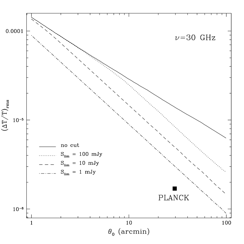
Figure 3: Fluctuations in the CMB anisotropy due to accretion flows in the cores of ellipticals, after removal of all sources above a flux $S_{\rm lim}$. Here a fraction $f=0.5$ of high-luminosity sources has been assumed in the sample.

Figure 3 shows, in the case of a fraction $f=0.5$ of high-luminosity sources in the sample, the expected level of fluctuations if all sources above a flux $S_{\rm lim}$ were individually identified and substracted out from the sample. This is shown for different choices of $S_{\rm lim}$. Identification and removal of individual sources can in principle be done by means of independent surveys.

Using the same parameters as in Figure 3, Figure 4 shows a comparison between the poissonian power spectrum (Eq. 6) produced by the accretion flows in ellipticals and the predicted power spectrum for a standard CDM model. The heavy solid line shows the contribution to the power spectrum from noise in the 30 GHz channel of the Planck LFI. Note that the “flat” ($C_{l}$ = constant) angular power spectrum of the fluctuations due to ADAF sources differs substantially from the power spectrum of primordial fluctuations. We find that the source signal is generally well below that of the intrinsic fluctuations, and it only becomes comparable to these on the small angular scales, where also the instrumental noise increases to roughly the same level. Removal of source signal should be possible even in cases where it gives a strong contribution. Even if the Poisson component of the sources and the noise due to the instrument have similar power spectra, they are indeed different in their nature (as emphasized by Scott & White 1999). In fact, while the sources on the sky contribute to the flux in every observation of a given pixel, the noise, on the other hand, differs from observation to observation, and, by assumption, it is uncorrelated with the signal in that pixel. Therefore, if a given direction in the sky is observed multiple times (as expected for Planck), the instrumental noise component can be separated from the sky signal.

5 DISCUSSION

We have computed the temperature fluctuations and power spectrum produced by inverted radio spectra from hot accretion flows in the nuclei of nearby elliptical galaxies in the Planck 30 GHz channel, where their emission is expected to peak. We have shown that the contribution from this class of sources approaches the intrinsic CMB fluctuation level only at small angular scales. However, because of the different nature of its power spectrum, the source contribution should not affect the most important goal of the Planck mission, that is the accurate measurement of the primary CMB anisotropy.

On the other hand, Planck will provide a large statistical sample of sources characterized by inverted spectra. Therefore, it should be possible to use this study to determine how common this mode of accretion is in the nearby supermassive black holes. In particular, as most of the contribution from this population is expected to peak at high radio frequencies, Planck should allow us to study their spectral characteristics. In turn, because different spectral distributions and luminosities reflect the shape of the density profiles, CMB experiments could allow us to gain important information on the physical conditions in these accretion flows. As already noted by Toffolatti et al. (1999b), the implications of such a study could, more generally, be significant as a way of testing the physical processes in the medium surrounding massive black holes, and the evolution of the interstellar medium in galaxies up to moderate redshifts. Even more, it would provide a test for current ideas according to which a significant fraction of the $X$-ray background may due to accretion in this regime in early-type galaxies in the local universe (Di Matteo & Allen 1999). Note that such a significant statistical study would be more difficult to carry out with surveys at other wavelengths because of the rapid decline of the ADAF flux, which makes the emission from this type of accretion flows extremely weak in the far infrared and optical bands.

We need to stress that, in principle, the contribution from ADAF sources should be easily disentangled not only from that due to sources with a flat and steep spectrum, but also from that due to GPS sources which also have strongly inverted spectra. GPS sources are typically much brighter (with fluxes typically ranging from a few to 10 Jy) but rarer (usually associated with QSOs) than the expected ADAF sources. The number of GPS sources rapidly decreases with decreasing flux, whereas ADAFs are expected to be much more numerous at faint flux levels. As a result, GPS are only minor contributors to the fluctuations at small angular scales, whereas ADAFs would be mostly significant at these scales. Therefore it should be possible to study these two populations independently.

Note that we have shown the expected temperature fluctuations due to ADAF sources only for the lowest energy channel of Planck. If most of the sources are indeed in the range of luminosities consistent with those observed so far, then this channel is expected to have the largest (possibly major) contribution, due to the high-frequency cutoff in the spectrum of these sources. However, if a substantial population of high-luminosity sources is present, then some contribution should also be present in the other channels of the Planck LFI. The availability of multifrequency data should allow an efficient identification of pixels contaminated by discrete sources. In order to carry out a substraction of the contaminating flux one should therefore take into account that strongly inverted spectra such as those considered here may not be present in most frequency channels but give rise to a strong contamination up to a certain frequency, and then abruptly drop. It should also be pointed out that, contrary to some of the GPS sources for which variability has been observed (e.g. Stanghellini et al. 1998), the radio sources in the hot accretion flows are usually not very variable. A lack of variability is particularly important for a proper removal of sources from the spectral fitting.

We note that ADAFs around massive black holes could also be found in spiral galaxies such as the Galactic nucleus Sgr A^∗. However, even if ADAFs were indeed common in spiral nuclei, their potential contribution to the CMB anisotropy would still be dominated by that from ellipticals. Inferred black hole masses are found to be proportional to the mass of the bulge component of their host galaxy, implying $M_{BH}\sim 10^{6}-10^{7}M_{\odot}$ for spiral galaxies. As a consequence, the contribution from spirals should be much lower, as the radio flux scales as $M_{\rm BH}^{2.5-3}$ (Franceschini et al. 1998), and (see §3) their spectrum would peak at frequencies higher than those of elliptical cores and affect higher energy (e.g. sub-mm, mm) channels of CMB experiments. Because of this, given enough sensitivity, the relevance of ADAFs in quiescent spiral nuclei may also be assesed separately by the forthcoming experiments.

Finally, we note that in our analysis we do not take into account the effects of source clustering. Clustering decreases the effective number of objects in randomly placed cells and, consequently, enhances the cell to cell fluctuations. There is indeed evidence that the positions in the sky of a wide variety of extragalactic sources are correlated (Shaver 1988). However, the specific correlation function of our radio–submm sources in early-type galaxies is not well-constrained. The analyses of Toffolatti et al. (1998) have shown that the contribution due to clustering (using the two-point correlation function from sources selected at 5 GHz; Loan, Wall & Lahav 1997) is generally small in comparison with the Poisson term; however, the relative importance of clustering increases if sources are substracted out from the Planck maps down to faint flux levels.

Figure 1: Synchrotron emission from low-radiative efficiency accretion flows. The various lines correspond to various amounts of mass loss in the flows ($p$ = 0, 0.2, 0.4, 0.6 from top to bottom). The uppermost curve is the standard ADAF model with no outflows. The shaded region indicates the range of luminosities which best fit the data in the cores of ellipticals observed so far (Di Matteo et al. 2000b).

Figure 2: Potential contribution to the CMB anisotropy from accretion flows in the cores of ellipticals as a function of the beamsize $\theta_{0}$ at $\nu=30$ GHz. The solid line shows the expected fluctuation level if the luminosities of all sources were in the range corresponding to the shaded region of Figure 1. The other lines show the fluctuations expected if a fraction $f$ of sources with a higher luminosity (corresponding to the uppermost curve of Figure 1) were mixed with these sources. The noise level indicated for Planck is the average $\Delta T/T$ per pixel for 1$\sigma$ detection after two full sky coverages.

Figure 4: Poisson component of the angular power spectrum of our sources for a range of flux cuts: $S_{\rm lim}=100$ mJy (dotted line), $S_{\rm lim}=10$ mJy (dashed line), $S_{\rm lim}=1$ mJy (dotted-dashed line). This is shown for the case where a fraction $f=0.5$ of high-luminosity sources is present in the sample. To compare with the level of primary anisotropy expected, the prediction for a standard CDM spectrum is also shown, normalized to COBE. The thick solid line is the expected contribution to the power spectrum from noise in the 30 GHz channel of the Planck LFI.

References

- (1)
- (2) Allen S.W., Di Matteo T., Fabian A.C., 2000, MNRAS, 311, 493
- (3)
- (4) Blandford, R. D. & Begelman, M. C. 1999, MNRAS, 303, L1
- (5)
- (6) Cavaliere, A. & Setti, G. 1976, A&A, 46, 81
- (7)
- (8) Condon, J. J. 1974, ApJ, 188, 279
- (9)
- (10) Cooray, A. R., Grego, L., Holzappel, W. L., Marshall, J., & Carlstrom, J. E. 1998, ApJ, 115, 1388
- (11)
- (12) De Zotti, G., Granato, G. L., Silva, L., Maino, D., & Danese, L. astro-ph/9912282
- (13)
- (14) Di Matteo T., Allen S.W., 1999, ApJ, 527, L21
- (15)
- (16) Di Matteo, T., Fabian, A. C., Rees, M. J., Carilli, C. L., Ivison, R. J. 1999, MNRAS, 305, 492
- (17)
- (18) Di Matteo, T., Quataert, E., Allen, S. W., Narayan, R., Fabian A. C., 2000a, MNRAS, 311, 507
- (19)
- (20) Di Matteo, T., Carilli, C.L., Fabian A.C., 2000b, ApJ, submitted
- (21)
- (22) Fabian A. C., Rees M. J., 1995, MNRAS, 277, L55
- (23)
- (24) Franceschini, A., Toffolatti, L., Danese, L. & De Zotti. G. 1989, ApJ, 344, 35
- (25)
- (26) Franceschini, A., Vercellone, S., & Fabian, A. C. 1998, MNRAS, 297, 817
- (27)
- (28) Gawiser, E., & Smoot, G. F. 1997, ApJ, 480, L1
- (29)
- (30) Guerra, E. J., Haarsma, D. B., Partridge, R. B. 1998, AAS, 193, 4003
- (31)
- (32) Igumenshchev, I. V. Abramowicz, M. A. 1999, MNRAS, 303, 309
- (33)
- (34) Kogut, A., et al. 1996, ApJ, 464, L5
- (35)
- (36) Loan, A. J., Wall, J. V. & Lahav, O. 1997, MNRAS, 286, 994
- (37)
- (38) Mahadevan, R. 1997, ApJ, 477, 585
- (39)
- (40) Magorrian, J. et al. 1998, AJ, 115, 2285
- (41)
- (42) Mather, J. C., Fixsen, D. J., Shafer, R. A., Mosier, C., & Wilkinson, D. T. 1999, ApJ, 512, 511
- (43)
- (44) Mushotzky, R.F., Cowie, L.L., Barger, A.J., Arnaud A., 2000, Nature, in press
- (45)
- (46) Narayan, R. & Yi, I. 1995, ApJ, 444, 231
- (47)
- (48) Narayan, R., Mahadevan, R., Quataert, E. 1998, Theory of Black Hole Accretion Disks, edited by Marek A. Abramowicz, Gunnlaugur Bjornsson, and James E. Pringle. Cambridge University Press, p.148
- (49)
- (50) Philips, R. B. & Mutel, R. L., 1982, A&A, 106, 21
- (51)
- (52) Rees M. J., Begelman M. C., Blandford R. D., Phinney E. S., 1982, Nature, 295, 17
- (53)
- (54) Scheuer, P. A. G. 1957, Proc. Cambridge Phil. Soc., 53, 764
- (55)
- (56) Scheuer, P. A. G. 1974, MNRAS, 166, 329
- (57)
- (58) Scott, D. & White, M. 1999, A&A, 346, 1
- (59)
- (60) Shaver, P. A. 1988, in ’IAU Symposium 130, Evolution of large Scale Structures in the Universe’, ed. J. Audouze, M.-C. pelletan, and A. Szalay (Dordrecht: Reidel)
- (61)
- (62) Slee O.B., Sadler E.M., Reynolds J.E., Ekers R.D., 1994, MNRAS, 269, 92
- (63)
- (64) Smoot, G. F., et al. 1992, ApJ, 396, L1
- (65)
- (66) Sokasian, A., Gawiser, E., & Smoot, G. F. 1998, ApJ submitted, astro-ph/9811311
- (67)
- (68) Stanghellini, C., O’Dea, C. P., Dallacasa, D., Baum, S. A., Fanti, R., & Fanti, C. 1998, A&AS, 131, 303
- (69)
- (70) Stone, J. M., Pringle, J. E. Begelman, M. C. 1999, MNRAS, 310, 1002
- (71)
- (72) Tegmark, M. & Efstathiou, G. 1996, MNRAS, 281, 1297
- (73)
- (74) Toffolatti, L., Gomez, F. A., De Zotti, G., Mazzei, P., Franceschini, A., Danese, L. & Burigana, C. 1999a, MNRAS, 297, 117
- (75)
- (76) Toffolatti, L., De Zotti, G., Argueso, F., & Burigana, C. astro-ph/9902343
- (77)
- (78) Wrobel J. M., 1991, AJ, 101, 12
- (79)
- (80) Yi, I., & Boughn, S. P. 1998, APJ, 499, 198
- (81)