Three Dimensional Radiative Transfer

Abstract

Radiative Transfer (RT) effects play a crucial role in the thermal history of the intergalactic medium. Here I discuss recent advances in the development of numerical methods that introduce RT to cosmological hydrodynamics. These methods can also readily be applied to time dependent problems on interstellar and galactic scales.

The physics of photoionized gases is of crucial importance and many astrophysical applications. As the hydrodynamic modeling of astronomical objects is advancing at a rapid pace we are also forced to consider the complex problem of three dimensional radiative transfer of ionizing radiation. I will report here on recent advances we have made in developing appropriate numerical techniques to achieve this goal. These methods are applicable for a wide range of problems. One particular issue that arises in the formation of the first generation of stars shall serve as motivation.

1 One Motivation: Structure Formation and the beginning of the bright ages

The atomic nuclei in the primordial gas (mostly hydrogen and helium) first (re)combined with electrons at a redshift $z\sim 1000$. From the study of absorption spectra of high redshift quasars we know that this then neutral gas must have been ionized prior to $z=5$. Most likely this reionization process was caused via photoionization by UV photons produced in proto galactic objects either by massive stars or by the accretion onto compact objects. The formation of these first objects in the universe and their potential impact on subsequent structure formation is a highly topical issue in physical cosmology to date. In our standard models of structure formation cosmological objects form via hierarchical build up from smaller pieces. The dynamics is controlled by gravity of a dominant cold dark matter (CDM) component. Baryons will fall into virializing CDM halos in which they may cool and possibly fragment to form stars. The lower limit on the masses of luminous objects that may be formed is determined by (1) the pressure of the primordial gas, which determines whether it can settle in the dark matter halo (2) the ability of the baryons to cool to collapse to stellar densities.

Both these issues depend sensitively on the presence of UV photons (see Abel and Haehnelt 1999, Haiman, Abel and Rees 1999, and references therein). Since the intergalactic medium (IGM) is initially optically thick to $h\nu>13.6$ eV photons ionization fronts will be formed around the first sources. Because we believe that the radiation is produced in structures condensed from the IGM by gravitational instability, the first UV photons will see a clumpy inhomogeneous IGM. As a consequence the time–varying ionized regions will have complex morphologies.

The above physical processes have prompted us to develop methods for the treatment of RT in three dimensional cosmological hydrodynamics. In the following we describe the conditions under which the cosmological RT becomes equivalent to classical RT. Then we go on to discuss some possible methods to solve the latter. In this contribution I will only give a brief overview of my and my collaborators work. However, note that also Razoumov and Scott (1999) offer a different approach. Gnedin (1999) chose to use dramatic simplifications constructed such as to mimic the expected effects of radiative transfer in order to study the reionization of intergalactic hydrogen.

2 Cosmological Radiative Transfer

The equation of cosmological radiative transfer in comoving coordinates (cosmological, not fluid) is:

$$\frac{1}{c}\frac{\partial I_{\nu}}{\partial t}+\frac{\hat{n}\cdot\nabla I_{\nu}}{\bar{a}}-\frac{H(t)}{c}(\nu\frac{\partial I_{\nu}}{\partial\nu}-3I_{\nu})=\eta_{\nu}-\chi_{\nu}I_{\nu}$$ (1)

where $I_{\nu}\equiv I(t,\vec{x},\vec{\Omega},\nu)$ is the monochromatic specific intensity of the radiation field, $\hat{n}$ is a unit vector along the direction of propagation of the ray; $H(t)\equiv\dot{a}/a$ is the (time-dependent) Hubble constant, and $\bar{a}\equiv\frac{1+z_{em}}{1+z}$ is the ratio of cosmic scale factors between photon emission at frequency $\nu$ and the present time t. The remaining variables have their traditional meanings (e.g, Mihalas 1978.) Equation (1) will be recognized as the standard equation of radiative transfer with two modifications: the denominator $\bar{a}$ in the second term, which accounts for the changes in path length along the ray due to cosmic expansion, and the third term, which accounts for cosmological redshift and dilution.

One could, in principle, attempt to solve equation (1) directly for the intensity at every point given the emissivity $\eta$ and absorption coefficient $\chi$. However, the high dimensionality of the problem (three positions, two angles, one frequency and time $=$ 7D!) not to mention the high spatial and angular resolution needed in cosmological simulations would make this approach impractical for dynamic computations. Therefore we proceed through a sequence of well-motivated approximations which reduce the complexity to a tractable level.

2.1 Local quasi–static Approximation

We begin by eliminating the cosmological terms and factors. That we can do this can be understood on simple physical grounds. Before the universe is reionized, it is opaque to H and He Lyman continuum photons. Consequently, ionizing sources are local to scales of interest, and not at cosmological distances. In particular this means that the term multiplicative term $\frac{H(t)}{c}$ which is simply the reciprocal of the Hubble horizon at the time $t$ will ensure the cosmological term to be small as long as the opacity is much smaller than the horizon scale. If this is not the case and we have a simulation box size much smaller than the mean free path than we are at the limit where the cosmological terms will modify the boundary values but still not be important as the photons transverse the box. Therefore, setting $\bar{a}\equiv 1$, equation (1) reduces to its standard, non-cosmological form:

$$\frac{1}{c}\frac{\partial I_{\nu}}{\partial t}+\hat{n}\cdot\nabla I_{\nu}=\eta_{\nu}-\chi_{\nu}I_{\nu}$$ (2)

where now $\nu$ is the instantaneous, comoving frequency.

Thinking of the special case of a point source that switches on instantaneously one realizes that initially the ionization front will always propagate at the speed of light. Eventually it slows down as the ’incoming flux’ of neutrals grows with the increasing ionization surface. This will ensure that eventually the light crossing time (1/(c times I-front distance)) will become much shorter than the timescales of change of the emissivities and absorption coefficient on the right hand side of equation (2). At this point an explicit integration can employ large time steps making the term $\frac{1}{c}\frac{\partial I_{\nu}}{\partial t}$ negligible. From this point of the evolution on it will suffice to solve the static classic equation of radiative transfer ,

$$\hat{n}\cdot\nabla I_{\nu}=\eta_{\nu}-\chi_{\nu}I_{\nu}.$$ (3)

3 Methods

3.1 Brute Force: Ray Tracing

Abel, Norman and Madau (1999) give a method that integrates this quasi–static approximation along rays casted from point–sources. That method has the particular advantage that it will ensure photon conservation independent of resolution by exploiting the known analytic solution of radiative transfer for a homogeneous slab.

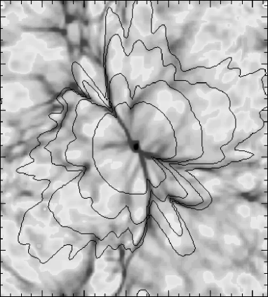
Figure 1: Propagation of an R-type I–front in a $128^{3}$ cosmological density field produced by a mini-quasar with $\dot{N}=5\times 10^{53}$s^-1. The solid contours give the position of the I–front at 0.15, 0.25, 0.38, and 0.57 Myr after the quasar has switched on. The underlying grey-scale image indicates the initial HI density field.

Consider the simple case of only absorption. Then across a computational cell where we assume the density of absorbing material to be constant the outgoing photon number flux is simple $e^{-\tau}$ times the incoming one. Hence the number of absorbed photons must be $(1-e^{-\tau})$ times the incoming flux. So one can compute the number of photoionizations per second by adding all these $(1-e^{-\tau})$ terms for the rays that pass this cell. Now by definition we ensure that the number of photoionizations will always equal the number of photons absorbed. As a consequence this method propagates ionization fronts at always the correct speed independent of resolution. This is a highly desirable feature of any method of multi-dimensional radiative transfer. This control of accuracy comes at high computational cost. In this method the $1/r^{2}$ drop in the photon flux in an optically thin region around the source is captured by the simple fact that many more rays traverse through cells near the source than cells further away. Obviously a large amount of computational time is wasted on computing the flux in such optically thin cell where it would simply be given by $I(0)/r^{2}$. This can be overcome as is discussed below. However, this method nevertheless can be used for a variety of realistic cases. This can be seen from Figure 1 and 2. Both of them employed the ray-tracing of Abel, Norman and Madau (1999) and are here shown as illustration of the practicality of this method.

3.2 Ionization Front tracking

Let us quickly side-track to point a simple way of solving a specific problem. If one is interested in the propagation of a R-type ionization front in a static medium it suffices to integrate the jump condition

$$n_{HI}(r)\frac{dR}{dt}=\frac{F(0)}{4\pi R^{2}}-\int_{0}^{R}\alpha(T(r))n_{HII}(r)n_{e}(r)dr,$$ (4)

where $R$, $\alpha$, and $F(0)$ denote the radius of the I-front, the recombination rate–coefficient, and the ionizing photon number luminosity, respectively. Dividing by $n_{HI}$ we can integrate equation (4) explicitly along rays and find the time at which the ionization fronts arrives at a given cell. Storing the arrival time in a 3D array allows one to investigate the time dependence morphology of ionization front by simply taking iso-surfaces on this array of arrival times. Such data is also interesting to compute how many ionizing photons are used to ionize a given volume in a static case, etc.. To get the full time evolution of the ionization front of one source on a 128³ numerical grid requires $\sim$ one minute computation (wall clock) on a workstation.

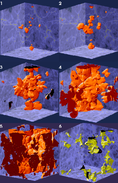
Figure 2: Visualization of a time series of a 3D radiative transfer simulation. Here we assumed 30 sources with an ionizing luminosity proportional to their halo mass that switch on simultaneously at redshift 7. The density distribution is take from a standard cold dark matter Lyman alpha forest simulation in a periodic box of 2.4 comoving Mpc carried out by Bryan et al. 1999. Hence the box corresponds to proper 300 kpc across. Six different panels are shown. Each slice at the cube edges illustrates the log of the hydrogen density. The iso–surfaces visualize the boundaries of ionized regions. The last panel, number six, illustrates remaining neutral islands that have not been ionized yet.

3.3 Computer Graphics

In many fields as e.g. biomedical imaging interactive volume rendering of 3 dimensional data is highly desirable. A lot of effort went into designing fast algorithms that yield optical depths from a light source and to the observers eye. Not any such method will be suitable for application in astrophysics in particular one needs to worry about exact photon (energy) conservation. However, imagine one has a method that gives the optical depth to a source at every point in the computational volume. For the case of pure attenuation one then also knows the photon number flux (photons per second per area) everywhere from

$$\vec{F}(\vec{r})=\frac{F_{source}(0)}{|\vec{r}|^{2}}\ e^{-\tau(\vec{r})}\frac{\vec{r}}{|\vec{r}|},$$ (5)

where $\vec{r}$ denotes the vector from the source to the point of interest. Now from the obvious ’discontinuity equation’:

$$\nabla\cdot\vec{F}(\vec{r})-\dot{n_{HI}}=0$$ (6)

one can ensure the number of photoionizations $\dot{n_{HI}}$ to be computed self–consistently independently of resolution. Such a method has been implemented and tested by Abel and Welling (2000) and found to give speed ups in excess of a factor hundred as compared to Abel, Norman and Madau (1999) in the limit of large ionized regions.

3.4 Moment Methods

The methods presented above focus and the correct implementation of radiative transfer for point sources. However, ideally we also want to be able to treat regions of diffuse emission as it arises e.g. due to bremsstrahlung and recombination radiation. In Norman, Paschos and Abel (1998) we have outlined a possibility approach to treat point sources and diffuse radiation by means of a variable Eddington tensor formalism. Although we have significantly improved on some ingredients of this method (as e.g. we derived an analytic expression for the Eddington tensors in the pre–overlap stage) we have not succeeded as yet in constructing a stable implementation.

4 Concluding Remarks

For the applications to numerical cosmology some of the methods of 3D radiative transfer discussed above will have to be combined. I-front tracking is useful to initialize the environment of new sources. The methods drawn from Computer Graphics can be used to compute accurate boundary conditions for the moment methods that are the most promising in the limit of many sources. A number of interesting problems still will need to be solved before cosmological radiation hydrodynamics can become a standard tool for the study of the formation and evolution of structure in the universe. However, the existing techniques should be employed for the study of interstellar problems in which only few sources are of interest. Planetary Nebulae and HII regions are ideal candidates for such three-dimensional radiation magneto–hydrodynamic modeling.

- [1] Abel, T., Norman, M.L., and Madau, P. 1999, ApJ, 520, 66.
- [2] Abel, T., Haehnelt, M. 1999, ApJL, 520, L13
- [3] Abel, T. 2000, in preparation.
- [4] Abel, T. and Welling, J. 2000, in preparation.
- [5] Bryan, G.L., Machacek, M., Anninos, P., Norman, M.L. 1999, ApJ, 517, 13
- [6] Gnedin, N. 2000, astro-ph/9909383, ApJ in press.
- [7] Haiman, Z., Abel, T., Rees, M.J. 2000, ApJ in press.
- [8] Norman, M. L., Paschos, P., & Abel, T. 1998, in “ in the Early Universe”, eds. F. Palla, E. Corbelli, and D. Galli, (Mem. S.A.It.), 271.
- [9] Razoumov, A. O., & Scott, D. 1999, MNRAS, 309, 287.