The neutrino star in the bulk Universe

Abstract

Motivated by the Kaluza-Klein theory with large extra spacetime dimensions the neutrino star built from the massive sterile neutrinos core and the massless brane neutrinos envelope is presented. The six-dimensional compactification scale $\sim 15$ MeV gives maximal neutrino mass $M_{max}=2.3\times 10^{4}\,M_{\odot}$with radius $R_{max}=1.2\times 10^{6}\,km$. The maximal neutrino star parameters varies with temperature. In the limit of the neutrino ball approximation the maximal sterile neutrino star is $M_{max}=1.1\times 10^{6}\,M_{\odot}$.

Introduction

Recently there has been considerable interest in the field theories with large extra spacetime dimensions. In the comparison to the standard Kaluza-Klein theory these extra dimensions may be restricted only to the gravity sector of theory while the Standard Model (SM) fields are assumed to be localized on the 4-dimensional spacetime 1 ,4 ,ADD3 .This is a promising scenario from the phenomenological point of view because it shift the energy scale of unification from $10^{19}\,GeV$ to $1-100\,TeV$. It has been recently shown L1 that this framework can be embedded into string models, where the fundamental Planck scale can be identified with the string scale which could be as low as the weak scale. The extra dimensions have the potential to lower the unification scale as well DDG1 .

The aim of this paper is to examine the degenerate neutrino star originated from the extra dimensional theory. The neutrino star ( neutrino ball ) was a subject of interest in the theory of the Standard Model hd . The fermion star in the extra dimensional theory was also the a subject of interest nk .The neutrino star model is capable to explain the nature of the object in Sgr A^∗ in the center of the Galaxy torr .

The bulk neutrino extension of the electroweak theory

Much of the interesting phenomenology of brane-world models is associated with the Kaluza-Klein theories tap that originate from large, gravity-only additional dimensions. The higher-dimensional bulk fermions lead to Kaluza-Klein towers of standard model singlets that may be interpreted as sterile neutrinos dinest ; ADDM ; dvali ; BCS . In this paper we shall consider the six-dimensional Kaluza - Klein theory. Let us now consider the action in the six-dimensional spacetime:

$${\mathcal{S}}=\int d^{6}x\sqrt{-g_{6}}L={\mathcal{S}}_{g}+{\mathcal{S}}_{F}=\int d^{6}x\sqrt{-g_{6}}(L_{g}+L_{F}),$$ (1)

where $g_{6}=det(g_{MN})$ and $M=\{\mu,\,i\}$, $N=\{\nu,\,j\}$ with $x^{M}=\{x^{\mu},y^{i}\},\,i=1,2$. The metrical tensor in the six-dimensional spacetime can be written:

$$g_{MN}=\left(\begin{array}[]{cc}e^{-2\xi(x)/f_{0}}\overline{g}_{\mu\nu}&0\\ 0&-\delta_{ij}e^{+2\xi(x)/f_{0}}\end{array}\right).$$ (2)

According to the above definition we can write:

$$\sqrt{-g_{6}}=\sqrt{-\overline{g}}e^{-2\xi(x)/f_{0}}.$$ (3)

We consider here the Lagrangian of the field as follows:

$$L=L_{g}+L_{F},$$ (4)

$$L_{g}=-\frac{1}{2\kappa_{6}}R,$$ (5)

$$L_{F}=L_{brane}\delta(y)+L_{bulk},$$ (6)

where $\kappa_{6}$ is the six-dimensional gravitational coupling. Its natural interpretation originates from the distance scaling in the four-dimensional spacetime. Let us compactify the six-dimensional spacetime $({\mathcal{M}}_{6}\rightarrow{\mathcal{M}}_{4}\times{\mathcal{S}}^{1}\times{\mathcal{S}}^{1})$ to the four-dimensional Minkowski one. In this paper we assume that the extra dimensions are compactified on the $2$ dimensional torus with a single radius $r_{2}$. The six-dimensional action may be rewritten as:

$${\mathcal{S}}=\int d^{4}x\int d^{2}y\sqrt{-g_{6}}L=\int d^{4}x\sqrt{-\overline{g}}{\mathcal{L}},$$ (7)

where $\int d^{2}y=(2\pi r_{2})^{2}$. The six-dimensional gravitional coupling $\kappa_{6}=8\pi G_{6}$ is convenient to define as

$$G_{6}^{-1}=\frac{4\pi}{(2\pi)^{2}}M^{4},$$

where $M$ - is the energy scale of the compactification ($\sim 10-100\,TeV$). Cosmological consideration hall gives the bound $M>100\,TeV$ what corresponds $r_{2}<5.1\times 10^{-5}\,mm$. If we define the four-dimensional coupling constant $\kappa=8\pi G_{N}=8\pi M^{-2}_{Pl}$ we get

$$M^{2}_{Pl}=4\pi M^{4}r_{2}^{2}.$$ (8)

The parameter $f_{0}$ is defined as:

$$f^{2}_{0}=\frac{1}{\pi}M^{2}_{Pl}$$ (9)

to produce the $1/2$ term in for the dilaton field kinetic term. The model can be motivated by the ten-dimensional string theory with the string scale $M_{s}$. For simplicity we assume that the first $2$ dimensions have the same size characterized by the radius $r_{2}$. This is likewise assumed for the remaining $4$ dimensions where the corresponding radius is called $r_{4}<r_{2}$. The four-dimensional Planck constant

$$(\frac{M_{Pl}}{M_{s}})^{2}=16\pi(2\pi r_{2}M_{s})^{2}(2\pi r_{4}M_{s})^{4}$$ (10)

is connected to the string scale $M_{s}$. In the result of the comparison to (8) we have

$$M=\sqrt{4\pi}(2\pi r_{4}M_{s})M_{s}.$$ (11)

The paremeters of the model karmen are presented on the Table 1.

	$M_{s}$	$M_{2}=r_{2}^{-1}$	$r_{4}^{-1}$	$M$
	$1.2$ TeV	$1.6$ MeV	$432.05$ MeV	$7.42\,10^{7}$ GeV
	$1.2$ TeV	$15$ MeV	$141.11$ MeV	$2.27\,10^{8}$ GeV

Table 1: The paremeters set of the model karmen .

In this section we shall extend the Standard Model minimally with the bulk neutrino $\psi(x,y)$. The lagrangian of the neutrino sector of the model is then:

$$L_{brane}=i\overline{L}_{f}\widehat{\Gamma}^{\mu}\partial_{\mu}L_{f}-\frac{1}{M_{s}}(h_{f,a}\overline{\psi}_{a}L_{f}H_{0}+h.c.),$$

and the fermion field are

$$L_{f}=\left(\begin{array}[]{c}\nu^{0}_{f}\\ 0\end{array}\right)_{L}\,\,\,f=e,\nu,\tau.$$ (12)

The Higgs field will have only the residual form

$$H_{0}=\frac{1}{\sqrt{2}}\left(\begin{array}[]{c}0\\ \upsilon\end{array}\right)$$ (13)

after the spontaneous symmetry breaking. The additional bulk neutrino is described by the Lagrange function

$$\mathcal{L}_{bulk} = i\overline{\psi}\widehat{\Gamma}^{N}\partial_{N}\psi-m_{D}(\overline{\psi}_{L}\psi_{R}+h.c),$$ (14)

where  $\psi_{R,L}=(I\pm\Gamma^{7})\psi$. The system has global $U(1)$ lepton symmetry which generates the lepton charge $Q_{L}$. The bulk neutrino field can be decomposed into four-dimensional Dirac spinors $\psi_{a}$, where $a=\{+,-\}$. The gamma matrices $\Gamma$ are defined as

$$\{\widehat{\Gamma}^{M},\widehat{\Gamma}^{N}\}=2g^{M,N}I.$$ (15)

In the flat four-dimensional spacetime, when $\overline{g}_{\mu\nu}=\eta_{\mu\nu}$ they may be defined as

$$\widehat{\Gamma}^{\mu}=e^{\xi/f_{0}}\Gamma^{\mu},\,\,\,\Gamma^{\mu}=\gamma^{\mu}\otimes I_{(2)},$$ (16)

$$\widehat{\Gamma}^{i}=e^{2\xi/f_{0}}\Gamma^{i},\,\,\,\Gamma^{i}=i\gamma^{5}\otimes\sigma^{i}$$

and

$$\{\gamma^{\mu},\gamma^{\nu}\}=2\eta^{\mu\nu}I,$$

$$\{\gamma^{i},\gamma^{j}\}=-2\delta_{i,j}I,$$

where

$$\Gamma^{7}=\overline{\Gamma}^{0}...\overline{\Gamma}^{5}=\gamma^{5}\otimes\sigma^{3},\,\,\,\,\gamma^{5}=-i\gamma^{0}\gamma^{1}\gamma^{2}\gamma^{3}.$$

Using the metric tensor six-dimensional form (2) and the (16) we can calculate the Lagrange function in the four-dimensional Minkowski spacetime

$$L=i\overline{L}\gamma^{\mu}D_{\mu}L+e^{-2\xi/f_{0}}\sum_{a,\underline{n}}i\overline{\psi}_{a,\underline{n}}(x)\gamma^{\mu}D_{\mu}\psi_{a,\underline{n}}(x)$$ (17)

$$-m_{D}\sum_{a,\underline{n}}\overline{\psi}_{a,\underline{n},L}\psi_{a,\underline{n},R}-e^{\xi/f_{0}}\sum_{a,\underline{n}}\overline{\psi}_{a,\underline{n}}(x)(\gamma^{i}u_{\underline{n}}^{i})\psi_{a,\underline{n}}(x),$$

where

$$u_{\underline{n}}^{i}=\frac{1}{r_{2}}n^{i},\,\,\,\,m^{2}_{\underline{n}}=\underline{u}^{2}_{\underline{n}}=m\frac{1}{r_{2}^{2}}(n_{1}^{2}+n_{2}^{2}).$$ (18)

The bulk neutrino is decomposed as

$$\psi_{a}(x,y)=\frac{e^{\xi/f_{0}}}{(2\pi r_{2})}\sum_{\underline{n}}\psi_{a,\underline{n}}(x)exp(\frac{1}{r_{2}}i\underline{n}\underline{y}).$$ (19)

Each of these four-dimensional Dirac spinors can be decomposed into Weyl spinors

$$\psi_{a,\underline{n}}(x)=\left(\begin{array}[]{c}\xi_{a,\underline{n}}^{c}\\ \eta_{a,\underline{n}}\end{array}\right).$$ (20)

After electroweak symmetry breaking we introduce the mass

$$m_{f,a}=\frac{h_{f,a}v}{2\pi(M_{s}r_{2})}\sim 10^{-1}\,\,MeV.$$ (21)

The exact diagonalization of the mass matrix gives three exactly massles Weyl fermions

$$\nu_{f}=U_{f,f^{\prime}}\nu^{0}_{f^{\prime}}+V_{f,a}(\underline{0})\eta_{a}(\underline{0})$$ (22)

and two Dirac spinors for each mode number $\underline{n}$ with mass

$$M_{\underline{n}}=\sqrt{m_{D}^{2}+m^{2}_{\underline{n}}}.$$ (23)

In general karmen , there is a superposition of the electroweak neutrinos $\nu^{0}_{f}$ on the brane and the Kaluza-Klein bulk neutrinos $\eta_{a}(\underline{n})$.

The neutrino star

An alternative model for the supermassive compact object in the center of our Galaxy has been recently proposed by Tsiklauri and Viollier rm tsi . The main ingredient of the proposal is that the dark matter at the center of the galaxy is non-baryonic composed with massive neutrinos or gravitinos. Such neutrino balls could have formed in early epochs, during a first-order phase transition in the Standard Model.

In case of the spherically symmertic gravitational field we have:

$$\overline{g}_{\mu\nu}=\left(\begin{array}[]{cccc}e^{\nu(r)}&&&\\ &-e^{\lambda(x)}&&\\ &&-r^{2}&\\ &&&-r^{2}\sin^{2}\theta\end{array}\right).$$ (24)

In the similar way the dilaton filed $\xi(r)$ will be dependent on the radius $r$. As $\xi(r)\sim f_{0}=M_{Pl}/\sqrt{\pi}\approx 10^{19}\,GeV$ we shall neglect the dilaton filed $\xi(r)$ in the first approximation. In this paper we present numerical results describing the structure of neutrino star. It is possible to describe a static spherical star solving the Oppenheimer-Tolman-Volkoff (OTV) equations (more general case with the dilaton filed $\xi(r)$ is presented in Appendix I).

$$\frac{dP(r)}{dr}=-\frac{G}{r^{2}}(\rho(r)+\frac{P(r)}{c^{2}})\frac{(m(r)+\frac{4\pi}{c^{2}}P(r)r^{3})}{(1-\frac{2Gm(r)}{c^{2}r})},$$ (25)

$$\frac{dm(r)}{dr}=4\pi r^{2}\rho(r).$$ (26)

Having solved the OTV equation the pressure $p(r)$, mass $m(r)$ and density $\rho(r)$ were obtained. To obtain the total radius $R$ of the star the fulfillment of the condition $p(R)=0$ is necessary. Our aim is to achieve the equation of state of neutrino star matter at finite temperature. In such a case the physical system can be defined by the thermodynamic potential $\Omega$ fet

$$\Omega=-k_{B}TlnTr(e^{-\beta(H-\mu Q_{L})}),$$ (27)

where $\beta=1/k_{B}T$, $k_{B}$ is the Boltzmann constant, $Q_{L}$ lepton charge. The chemical potential $\mu$ reflects the lepton number conservation. $H$ stands for the Hamiltonian of the physical system. All needed averages are calculated with the Hamiltonian $H$. We define the density of energy and pressure by the energy - momentum tensor

$$T_{\mu\nu}=(P+\epsilon)u_{\mu}u_{\nu}-Pg_{\mu\nu},$$ (28)

where $u_{\mu}$ is a unite vector ($u_{\mu}u^{\mu}=1$). So, the calculations give

$$\epsilon(x_{F},T)=\rho c^{2}=\epsilon_{F,bulk}+\epsilon_{F,brane},$$ (29)

$$P(x_{F},T)=P_{F,bulk}+P_{F,brane},$$ (30)

where

$$\epsilon_{F}=\epsilon_{0}\chi(x_{F},T),$$ (31)

$$P_{F}=P_{0}\phi(x_{F},T).$$ (32)

The fact that the bulk Dirac neutrinos are massive means that they play the same role like ions in a white dwarf or neutrons in a neutron star. We have

$$\chi_{bulk}(x_{F},T)=\frac{1}{{}^{\pi^{2}}}\int_{0}^{\infty}dz\,z^{2}\sqrt{z^{2}+1}\{\frac{1}{\exp((\sqrt{1+z^{2}}-\mu^{\prime})/\tau)+1}$$ (33)

$$+\frac{1}{\exp((\sqrt{1+z^{2}}+\mu^{\prime})/\tau)+1},$$

$$\phi_{bulk}(x_{F},T)=\frac{1}{3\pi^{2}}\int_{0}^{\infty}\frac{z^{4}dz}{\sqrt{z^{2}+1}}\{\frac{1}{\exp((\sqrt{1+z^{2}}-\mu^{\prime})/\tau)+1}$$ (34)

$$+\frac{1}{\exp((\sqrt{1+z^{2}}+\mu^{\prime})/\tau)+1}\},$$

where $\tau=(k_{B}T)/M_{2}$,

$$\mu^{\prime}=\mu/M_{2}=\sqrt{1+x_{F}^{2}}$$ (35)

and

$$x_{F}=k_{F}/M_{s}.$$ (36)

Similarly to the paper toki we have introduced (35,36) the dimensionless “Fermi” momentum even at finite temperature which exactly corresponds to the Fermi momentum at zero temperature. For the massless brane neutrinos we have

$$\chi_{brane}(x_{F},T)=\frac{\gamma}{2\pi^{2}}\int dz\,z^{3}\{\frac{1}{(e^{(z-x_{F})/\tau}+1)}+\frac{1}{(e^{(z+x_{F})/\tau}+1)}\}$$ (37)

$$=-\frac{3\gamma}{\pi^{2}}t^{4}\int^{\infty}_{0}\frac{dz\,z^{3}}{e^{(z-x_{F})/\tau}+1}\left\{Li_{4}(e^{x_{F}/\tau})+Li_{4}(e^{-x_{F}/\tau})\right\},$$ (38)

where the presure is

$$\phi_{brane}(x_{F},T)=\frac{1}{3}\epsilon_{brane}(x_{F},T).$$ (39)

Both $\epsilon_{F}$ and $P_{F}$ depend on the neutrino chemical potential $\mu$ or Fermi momentum $x_{F}$. This parametric dependence on $\mu$ (or $x_{F}$) defines the equation of state.

Similarly to the paper toki we have introduced the dimensionless ’Fermi’ momentum even at finite temperature which exactly corresponds to the Fermi momentum at zero temperature. Both $\epsilon_{F}$ and $P_{F}$ depend on the neutrino chemical potential $\mu$ or Fermi momentum $x_{F}$. This parametric dependence on $\mu$ (or $x_{F}$) defines the equation of state.

When Fermi momentum reaches the second Kaluza-Klein level $\sim m_{D}\sqrt{2}$ the number of avaliable neutrino modes will change. For the high bulk neutrino density in the ultrarelativistic limit all Kaluza-Klein modes should be included. In that limit energy density of the bulk neutrinos is equal to

$$\chi_{bulk}(x_{F},T)=\frac{\gamma}{3\pi^{2}}(r_{2}M_{2})\int dz\,z^{5}\{\frac{1}{(e^{(z-x_{F})/\tau}+1)}+\frac{1}{(e^{(z+x_{F})/\tau}+1)}\}$$ (40)

$$=-\frac{40\gamma}{\pi}(r_{2}M_{2})t^{6}\int^{\infty}_{0}\frac{dz\,z^{5}}{e^{(z-x_{F})/\tau}+1}\left\{Li_{6}(e^{x_{F}/\tau})+Li_{6}(e^{-x_{F}/\tau})\right\}.$$ (41)

In the ultrarelativistic limit the equation of state is

$$\phi_{bulk}(x_{F},T)=\frac{1}{5}\epsilon_{bulk}(x_{F},T).$$ (42)

The equations (25,26) are easy integrated numerically, For example, for the neutron star with the central density $\rho_{c}=\,10^{4}\,g/cm^{3}$ and temperature $T=50\,keV$ the star density and pressure profile are presented on the Fig.1 and Fig. 2. Similarly to a structure of white dwarf massive sterile neutrinos like ions contribute to the density of the star , while the massles neutrinos like electrons contribute to the pressure. This feature will be more visible with the increasing temperature.

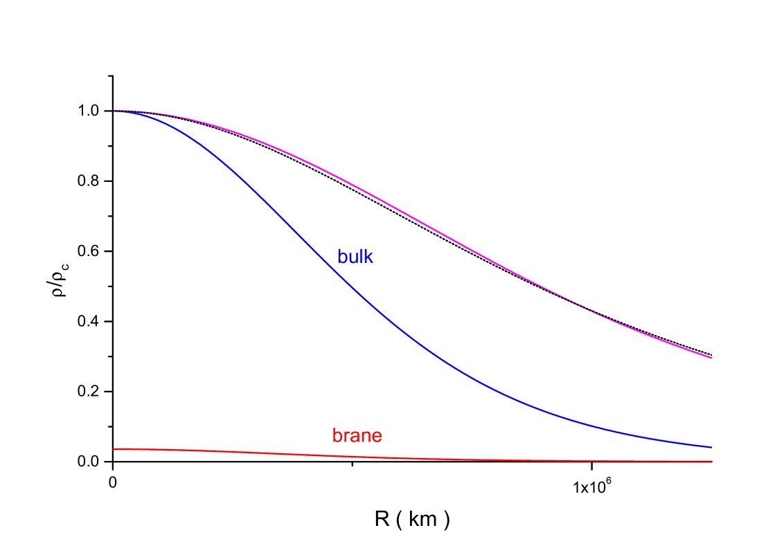
Figure 1: The density profile of the neutrino star for the bulk neutrino (blue), brane ones (red), in the ultrarelativistic limit (magenta) and in the neutrino ball case (the dot line).

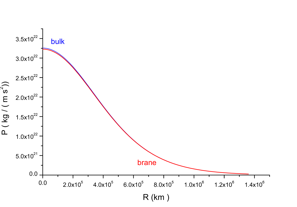
Figure 2: The pressure profile of the neutrino star.

The parameters of the maximum mass configuration are:

$$M_{max}=2.3\times 10^{4}\,M_{\odot},\,\,\,R=1.2\times 10^{6}\,km.$$ (43)

This fact is easy to notice on the mass-radius diagram (Fig. 3). In general, we have all family of neutrino stars, depending on growing neutrino Fermi momentum. This result concerns the Ferni momentum below the second Kaluza-Klein level $\sim m_{D}\sqrt{2}$ . The ulrarelativistic limit gives higher masses $M_{max}\sim 1.6\times 10^{6}\,M_{\odot}$. The density profile in this limit is presented on the Fig 1 (magenta). In limit of bulk neutrino ball (Appendix I) the neutrino star properties are presented in Table 2.

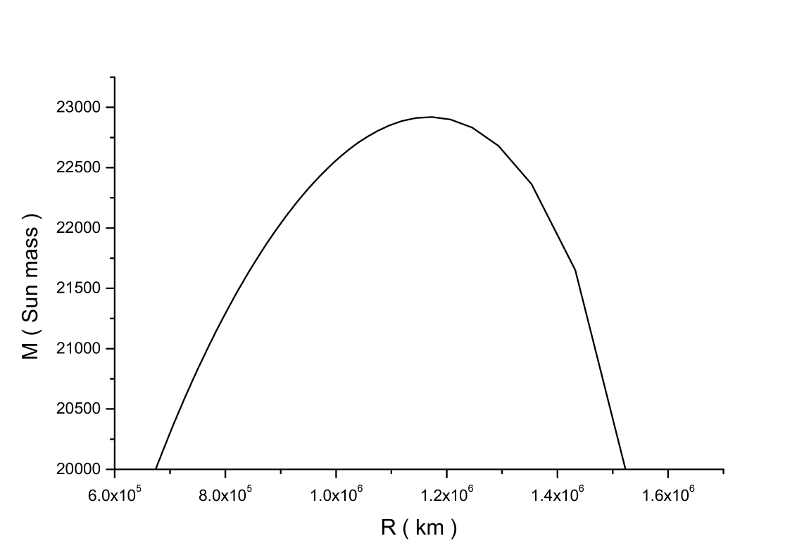
Figure 3: The R-M diagram for the neutrino star.

and the neutrino star mass dependence from the central density $\rho_{c}$ (Fig. 4).

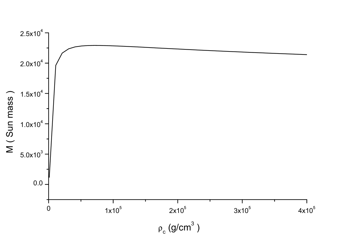
Figure 4: The neutrino star mass dependence from the central density $\rho_{c}$.

Appendix

The Einstein equations in in the six-dimensional spacetime (the metric tensor (2,24) ) can be written as

$$e^{-\lambda(r)}(\frac{\nu^{\prime}(r)}{r}+\frac{1}{r^{2}}-2\frac{\xi^{\prime}(r)^{2}}{f_{0}^{2}})-\frac{1}{r^{2}}=\frac{8\pi G_{6}}{c^{4}}e^{-2\xi(r)/f_{0}}P(r),$$ (44)

$$e^{-\lambda(r)}(-\frac{\lambda^{\prime}(r)}{r}+\frac{1}{r^{2}}+2\frac{\xi^{\prime}(r)^{2}}{f_{0}^{2}})-\frac{1}{r^{2}}=-\frac{8\pi G_{6}}{c^{2}}e^{-2\xi(r)/f_{0}}\rho(r).$$ (45)

The Einstein equations give also the equation for the dilaton field:

$$\xi^{\prime\prime}(r)+\frac{2}{r}\xi^{\prime}(r)-\frac{1}{2}\xi^{\prime}(r)(\lambda^{\prime}(r)-\nu^{\prime}(r))-\frac{1}{f_{0}}\xi^{\prime}(r)^{2}+$$ (46)

$$f_{0}(\frac{1}{2r^{2}}(e^{\lambda(r)}-1)+\frac{1}{2r}(\lambda^{\prime}(r)-\nu^{\prime}(r))+\frac{1}{8}(\lambda^{\prime}(r)-\nu^{\prime}(r))\nu^{\prime}(r)-$$

$$\frac{1}{4}\nu^{\prime\prime}(r)+\frac{4\pi G_{6}}{c^{4}}e^{\lambda(r)-2\xi(r)/f_{0}}\,P_{s}(r)).$$

The continuity equation $T^{MN}_{;M}=0$ gives

$$\nu^{\prime}(r)=-\frac{2P^{\prime}(r)}{(P+c^{2}\rho)}-2\frac{\xi^{\prime}(r)}{f_{0}}\,\frac{(P-2P_{s}-c^{2}\rho)}{(P+c^{2}\rho)}.$$ (47)

We assume that the energy-momentum tensor has a diagonal form $diag(T_{\mu\nu})=\{\varepsilon,P,P,P,P_{s},P_{s}\}$. Integrating of equation (45) yields we can write:

$$e^{-\lambda(r)}=\frac{\int\frac{dr}{r}((1-\frac{8\pi G}{c^{2}}r^{2}\rho(r)\,e^{-\frac{2\xi(r)}{f_{0}}})\,e^{\int dr(\frac{1}{r}+\frac{2r}{f_{0}^{2}}\xi^{\prime}(r)^{2})})}{\exp(\int dr(\frac{1}{r}+\frac{2r}{f_{0}^{2}}\xi^{\prime}(r)^{2}))}.$$ (48)

If we define

$$e^{-\lambda(r)}=1-\frac{2G_{6}}{c^{2}r}m(r),$$ (49)

then we can obtain the generalized Oppenheimer-Tolman-Volkoff equation:

$$\frac{dP(r)}{dr}=-\frac{G_{6}}{r^{2}}\frac{(\rho(r)+\frac{P(r)}{c^{2}})(m(r)+\frac{4\pi}{c^{2}}P(r)r^{3}\,e^{-2\xi(r)/f_{0}})}{(1-\frac{2G_{6}}{c^{2}r}m(r))}+$$ (50)

$$(\frac{\xi^{\prime}(r)^{2}}{f_{0}^{2}}-\frac{\xi^{\prime}(r)}{{}^{f_{0}}}\frac{(P-2P_{s}-c^{2}\rho)}{(P+c^{2}\rho)})\,(c^{2}\rho+P).$$ (51)

In vacuum $P=0\,,\,P_{s}=0$, of course we have well known Schwarzschild solution:

$$e^{-\lambda(r)}=(1-\frac{r_{g}}{r}),$$

$$e^{\nu(r)}=(1-\frac{r_{g}}{r}),$$

$$\xi(r)=0.$$

Neglecting the dilaton field $\xi(r)$ the Oppenheimer-Tolman-Volkoff (25).

The theory of neutrinos, bound by gravity, can be easily sketched considering a Thomas-Fermi model for fermions bilic . We can set the Fermi energy equal to the gravitational potential which binds the system, and see that the number density is a function of the gravitational potential. Such a gravitational potential will obey a Poisson equation, where neutrinos (and anti-neutrinos) are the source term. Including gravity the local equilibrium condition demands

$$\frac{1}{r^{2}}\frac{d}{dr}(\frac{r^{2}}{\rho(r)}\frac{dp}{dr})=-4\pi G_{N}\rho(r).$$ (52)

Inside the ball the pressure of the massive bulk neutrinos is $P=\rho/5$ while $P=\rho/3$ for the brane neutrinos in the relativistic limit in high temperature. Defining

$$\rho(r)=\rho_{c}e^{\varphi}$$ (53)

with

$$\kappa=24\pi G_{N}\rho_{c}$$ (54)

we have the Liuoville equation

$$\triangle\varphi=-\kappa e^{\varphi}.$$ (55)

The Laplace operator is

$$\triangle=\frac{1}{r^{2}}\frac{d}{dr}(r^{2}\frac{d}{dr})+...$$ (56)

Using the thin-wall approximation one can obtain the following expression

$$F_{0}(r)=e^{\phi}=\frac{1}{{\cosh}^{2}(\frac{\sqrt{2\kappa}}{2}r)}.$$ (57)

The equation (57) allows to estimate the mass of the neutrino ball which is given by the dependence

$$M(R)=4\pi\rho_{c}\int_{0}^{\infty}\frac{drr^{3}}{{\cosh}^{2}(\frac{\sqrt{2\kappa}}{2}r)}$$ (58)

with the radius scale

$$r_{0}=\sqrt{\frac{\kappa}{2}}.$$ (59)

The bulk neutrino density profile (57) is presented on the Fig. 1 (the dotted line).

$\rho_{c}\,(g/cm^{3})$	$R\,(km)$	$M\,(M_{\odot})$
$10^{3}$	$5.9\,10^{6}$	$1.1\,10^{6}$
$10^{4}$	$1.8\,10^{6}$	$3.5\,10^{5}$
$10^{5}$	$5.9\,10^{5}$	$1.1\,10^{5}$

Table 2: The bulk neutrino star properties in the neutrino ball approximation.

References

• (1) N. Arkani-Hamed, S. Dimopoulos, and G. Dvali, Phys. Lett. B429, 263 (1998).
• (2) I. Antoniadis, N. Arkani-Hamed, S. Dimopoulos, and G. Dvali, Phys. Lett. B436, 257 (1998).
• (3) N. Arkani-Hamed, S. Dimopoulos, and G. Dvali, Phys. Rev. D59, 086004 (1999).
• (4) J. Lykkin, Talk at the International Workshop on Phenomenological Aspects of Superstring Theories (PAST97), Trieste, Italy, 2-4 October, 1997.
• (5) K.R. Dienes, E. Dudas, and T. Gherghetta, Phys. Lett. B436, 55 (1998).
• (6) B.Holdom, Phys. Rev. D36, 1000 (1987);
• (7) D.F.Torres, S.Cappozziello, G. Lambiase, A supermassive scalar star at the Galactic Center?, http://xxx.lanl.gov/abs/astro-ph/0004064.
• (8) N. Kan, K. Shiraishi, Fermion star with an Extra Dimension, http://xxx.lanl.gov/abs/gr-qc/0001027.
• (9) T.Appelquist, A.Chodos, P.G.O. Freund Modern Kaluza-Klein Theories, Addison-Wesley Publishing Comp. Meno Park, 1987.
• (10) K. R. Dienes, E. Dudas, and T. Gherghetta, Neutrino oscillations without neutrino masses or heavy mass scales: A higher-dimensional seesaw mechanism, Nucl. Phys. B557 25 (1999); http://xxx.lanl.gov/abs/hep-ph/9811428,http://xxx.lanl.gov/abs/hep-ph/9811428.
• (11) N. Arkani-Hamed, S. Dimopoulos, G. Dvali, and J. March-Russell, Neutrino masses from large extra dimensions, http://xxx.lanl.gov/abs/hep-ph/9811448, http://xxx.lanl.gov/abs/hep-ph/9811448.
• (12) G. Dvali and A. Y. Smirnov, Probing large extra dimensions with neutrinos, Nucl. Phys. B563 63 (1999),http://xxx.lanl.gov/abs/hep-ph/9904211.
• (13) R. Barbieri, P. Creminelli, and A. Strumia, Neutrino oscillations from large extra dimensions, http://xxx.lanl.gov/abs/hep-ph/0002199.
• (14) L.J. Hall, D. Smith, Constraints on Theories with Large Extra Dimensions, http://xxx.lanl.gov/abs/hep-ph/9904267, Phys. Rev. D60, 085008 (1999).
• (15) A. Lukas, A. Romanino, A Brane-World Explanation of the KARMEN Anomaly, http://xxx.lanl.gov/abs/hep-ph/0004130.
• (16) R.Mańka, I.Bednarek, D.Karczewska, The neutrino ball in the standard model. http://xxx.lanl.gov/abs/astro-ph/9304007; Phys. Scr. 52, 36 (1995); R.Mańka, D.Karczewska, Z. Phiz. C57, 417 (1993).
• (17) Tsiklauri D., and Viollier R. D., ApJ., 500, 591 1998;
• (18) A.L.Fetter, J.D.Walecka, Quantum Theory of Many-Particle Systems, McGraw-Hill, New York, 1971.
• (19) K.Sumiyoshi, H.Toki, ApJ, 422, 700 1994.
• (20) N.Bilic, D.Tsiklauri, R.Viollier, Prog. Part. Nucl. Phys. 40, 17 (1998).