Presupernova Evolution of Rotating Massive Stars II:
Evolution of the Surface Properties

Abstract

We investigate the evolution of the surface properties of models for rotating massive stars, i.e., their luminosities, effective temperatures, surface rotational velocities, and surface abundances of all isotopes, from the zero age main sequence to the supernova stage. Our results are based on the grid of stellar models by Heger et al. (2000), which covers solar metallicity stars in the initial mass range $8-25\,{\mathrm{M}_{\odot}}$. Results are parameterized by initial mass, initial rotational velocity and major uncertainties in the treatment of the rotational mixing inside massive stars.

Rotationally induced mixing processes widen the main sequence and increase the core hydrogen burning lifetime, similar to the effects of convective overshooting. It can also significantly increase the luminosity during and after core hydrogen burning, and strongly affects the evolution of the effective temperature. Our models predict surface rotational velocities for various evolutionary stages, in particular for blue supergiants, red supergiants, and for the immediate presupernova stage.

We discuss the changes of the surface abundances due to rotationally induced mixing for main sequence and post main sequence stars. We single out two characteristics by which the effect of rotational mixing can be distinguished from that of massive close binary mass transfer, the only alternative process leading to non-standard chemical surface abundances in massive stars. A comparison with observed abundance anomalies in various types of massive stars supports the concept of rotational mixing in massive stars and indicates that it is responsible for most of the observed abundance anomalies.

1 Introduction

Massive main sequence stars are rapid rotators. Equatorial rotation velocities span the range ${v_{\mathrm{rot}}}=100-400\,{{\mathrm{km}}\,{\mathrm{s}}^{-1}}$, with B stars rotating closest to their break-up speed, ${v_{\mathrm{crit}}}$ Fukuda (1982); Howarth et al. (1997).

To date, stellar rotation and, in particular, rotationally induced mixing have not been taken into account in extended studies of nucleosynthesis in massive stars. However, it is required to reproduce, e.g., observed surface abundance anomalies of massive stars. In the present paper we predict the temporal evolution of the surface properties of rotating massive stars. This is of particular interest, as it allows a direct comparison of these models with observations.

Besides abundance changes, lifetime and evolution in the Hertzsprung-Russell (HR) diagram of rotating stars differ from those of non-rotating stars. This is particularly interesting for age determinations of young stellar clusters. Since appropriate sets of rotating stellar models have not been available so far, these studies have mostly neglected effects of rotation.

The calculations presented here treat rotation in stars according to the numerical method introduced by Endal & Sofia (1976, 1978); Pinsonneault et al. (1989). Our implementation is described in more detail in Heger et al. (2000). The results presented in this paper are based on calculations using the STERN code which contains a $36$ isotope network including all stable isotopes up to silicon. As in Heger et al. (2000), we concentrate on Type II supernova progenitor stars, i.e., stars which evolve sufficiently massive cores to become core-collapse supernovae, but not massive enough to experience sufficient mass loss (or mixing) to become Wolf-Rayet stars (i.e., initial masses in the range $\sim 8-20\,{\mathrm{M}_{\odot}}$). We also do not consider binaries.

A list of our initial models and the evolution of stellar structure and angular momentum in the stellar interior are given in Heger et al. (2000). The discussion of the observable stellar properties, which is the topic of the present paper, is divided in two major parts: the main-sequence evolution (§2) and the post-main sequence evolution (§3). In §4 we compare our results to observations and give our conclusions in §5.

2 Central hydrogen burning

Core hydrogen burning comprises about $90\,\%$ of the total stellar lifetime and is therefore the evolutionary phase which can be most easily compared with observations.

2.1 Nucleosynthesis and envelope abundances

Central hydrogen burning in massive stars is governed by the CNO cycle Bethe (1939); Clayton (1968). Equilibrium mass fraction ratios of roughly $1:50-100:1-5$ for ${{{\mathrm{}}}{{\mathrm{{}^{12}}}}{\mathrm{C}}}$ $:$${{{\mathrm{}}}{{\mathrm{{}^{14}}}}{\mathrm{N}}}$ $:$${{{\mathrm{}}}{{\mathrm{{}^{16}}}}{\mathrm{O}}}$ are established in the core Arnould & Mowlavi (1993). This deviates distinctly from typical initial ratios of about $1:0.3:3$ Grevesse & Noels (1993). Most of the initial carbon and oxygen is converted into ${{{\mathrm{}}}{{\mathrm{{}^{14}}}}{\mathrm{N}}}$. A subcycle of the CNO process, which transforms the initial ${{{\mathrm{}}}{{\mathrm{{}^{16}}}}{\mathrm{O}}}$ into ${{{\mathrm{}}}{{\mathrm{{}^{14}}}}{\mathrm{N}}}$, passes through ${{{\mathrm{}}}{{\mathrm{{}^{17}}}}{\mathrm{F}}}$ and ${{{\mathrm{}}}{{\mathrm{{}^{17}}}}{\mathrm{O}}}$ and is responsible for the production of ${{{\mathrm{}}}{{\mathrm{{}^{17}}}}{\mathrm{O}}}$. Further characteristic properties of the CNO cycle are the production of ${{{\mathrm{}}}{{\mathrm{{}^{13}}}}{\mathrm{C}}}$ and the destruction of ${{{\mathrm{}}}{{\mathrm{{}^{15}}}}{\mathrm{N}}}$.

In the stellar layers above the convective core the CNO equilibrium abundances are not reached. In particular, there is almost no processing of hydrogen into helium. However, isotopes which are produced at lower temperatures than where they are destroyed (e.g., ${{{\mathrm{}}}{{\mathrm{{}^{13}}}}{\mathrm{C}}}$ and ${{{\mathrm{}}}{{\mathrm{{}^{17}}}}{\mathrm{O}}}$) can have abundance maxima in the envelope.

Other nuclear cycles occurring during hydrogen burning involve, e.g., neon, sodium, magnesium, and aluminum. They do not contribute significantly to the energy generation, but they do alter the abundances of the involved isotopes. As the abundance changes of different isotopes occur at different temperatures, measuring their abundances at the stellar surface may contribute additional information about the mixing processes in the stellar interior.

The light isotopes ${{{\mathrm{}}}{{\mathrm{{}^{3}}}}{\mathrm{He}}}$, ${{{\mathrm{}}}{{\mathrm{{}^{6}}}}{\mathrm{Li}}}$, ${{{\mathrm{}}}{{\mathrm{{}^{7}}}}{\mathrm{Li}}}$, ${{{\mathrm{}}}{{\mathrm{{}^{9}}}}{\mathrm{Be}}}$, ${{{\mathrm{}}}{{\mathrm{{}^{10}}}}{\mathrm{B}}}$, and ${{{\mathrm{}}}{{\mathrm{{}^{11}}}}{\mathrm{B}}}$ are destroyed at the low temperature in the stellar envelope. This allows to use them to constrain mixing processes in the upper part of the envelope. For example, the surface depletion of lithium is applied to investigate models for the present sun Talon & Charbonnel (1998).

2.2 Internal mixing: the example of $\mathbf{20\,{\mathbf{M_{\odot}}}}$ stars

2.2.1 Mixing and barriers

Fig. 1 compares the internal abundance profiles of the most abundant isotopes as a function of the Lagrangian mass coordinate, $m$, in a non-rotating and two rotating $20\,{\mathrm{M}_{\odot}}$ models at core hydrogen exhaustion. The flat profiles in the innermost few solar masses are caused by convection. Small convective and/or semiconvective regions Heger et al. (2000) cause the “steps” in the profile above the convective core.

Fig. 1 also shows the absence of mixing above this region in the non-rotating case, visible as a kink in the hydrogen, helium, and oxygen profiles at about $m=10\,{\mathrm{M}_{\odot}}$. Between $m=10\,{\mathrm{M}_{\odot}}$ and $m=13\,{\mathrm{M}_{\odot}}$, a sharp decrease in ${{{\mathrm{}}}{{\mathrm{{}^{12}}}}{\mathrm{C}}}$ occurs, accompanied by an increase in ${{{\mathrm{}}}{{\mathrm{{}^{14}}}}{\mathrm{N}}}$. This is due to partial CNO processing “in place”, i.e., without any transport. Deeper in the core, the carbon mass fraction increases again and reaches its equilibrium value. Below $m=10\,{\mathrm{M}_{\odot}}$ ${{{\mathrm{}}}{{\mathrm{{}^{14}}}}{\mathrm{N}}}$ approaches its CNO equilibrium value, while oxygen is depleted. There is no thermonuclear depletion of oxygen above $m=10\,{\mathrm{M}_{\odot}}$. Above $m\approx 14\,{\mathrm{M}_{\odot}}$, the CNO isotopes retain their initial mass fractions.

In contrast, the rotating models show mixing of thermonuclear processed matter up to the surface of the star. In Model E20 (Fig. 1a; no inhibiting effects of gradients in the mean molecular weight ($\mu$-gradients) on the rotationally induced instabilities) an extended helium gradient reaches from the upper edge of the convective core up to the surface. Along with helium, also nitrogen is enriched while carbon and oxygen are depleted. Between $m=5\,{\mathrm{M}_{\odot}}$ and $m=10\,{\mathrm{M}_{\odot}}$, carbon is enhanced.

If $\mu$-gradients are allowed to inhibit the rotationally induced instabilities (Model E20B; Fig. 1b), the $\mu$-gradient which forms at the upper edge of the convective core is not smoothed out, but instead almost completely chokes off any mixing between core and envelope quite early during the evolution. Above the “barrier” due to the $\mu$-gradient ($\mu$-barrier), however, mixing is efficient (Fig. 1b). It’s stronger than for Model E20, since the efficiency for compositional mixing was assumed to be ${f_{\mathrm{c}}}=1/30$ in Model E20B instead of ${f_{\mathrm{c}}}=1/100$ for Model E20 Heger et al. (2000). Therefore, a stronger enrichment of nitrogen close to the surface results in Model E20B, due mainly to the processing of carbon into nitrogen. The ${{{\mathrm{}}}{{\mathrm{{}^{16}}}}{\mathrm{O}}}$ abundance in the envelope hardly changes in Model E20B, because the temperature above the $\mu$-barrier is never high enough to allow for its processing. Helium, being the main reason for the $\mu$-barrier, remains small in the envelope.

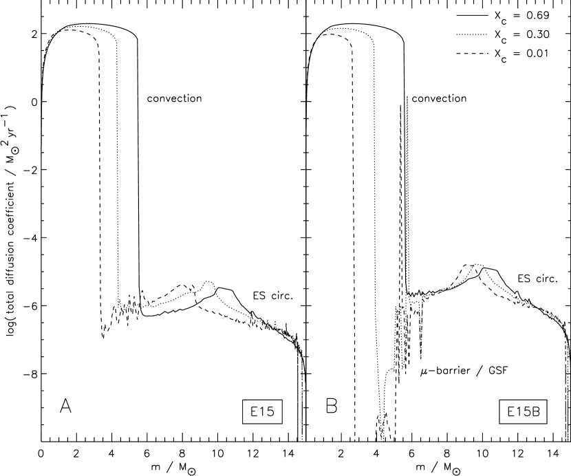
Figure 2: Total diffusion coefficient for chemical mixing as a function of mass coordinate, $m$, at three different stages of central hydrogen burning: 1 % of central hydrogen, by mass, burnt (${X_{\mathrm{c}}}=0.69$; solid line), and at central hydrogen mass fractions of 30 % (${X_{\mathrm{c}}}=0.30$; dotted line) and 1 % (${X_{\mathrm{c}}}=0.01$; dashed line). Panel a: Model E15, rotationally induced mixing is not inhibited by $\mu$-gradients. Panel b: Model E15B, rotationally induced mixing is (slightly; ${f_{\mathrm{\mu}}}=0.05$) inhibited by $\mu$-gradients. The labels in the figure indicate the regime of diffusion coefficient for convection and Eddington-Sweet circulation (ES circ.). For Model E15B, the $\mu$-barrier is indecated. In that region, the Eddington-Sweet circulation is inhibited and the Goldreich-Schubert-Fricke instability (GSF) is most efficient process. Note the region of essentially no mixing above the central convection zone for the two evolved stages (${X_{\mathrm{c}}}=0.30$, $0.01$) of Model E15B.

In Fig. 2 we show the total diffusion coefficient as resulting from all mixing processes taken into account at the beginning, about the middle, and the end of central hydrogen burning for Models E15 and E15B. For Model E15B the $\mu$-barrier can be seen a deep drop in the diffusion coefficient above the convective core at the two later times, while the $\mu$-barrier is not yet present at the beginning of core hydrogen burning (solid line). In Model E15 such a $\mu$-barrier never forms, since the rotationally induced mixing is assumed insensitive to $\mu$-gradients, and thus material from the core can be mixed up to the surface during whole central hydrogen burning. However, note that the diffusion coefficient by rotationally induced mixing processes, dominated by Eddington-Sweet circulation in the envelope, is lower by a factor three compared to Model E15B, since ${f_{\mathrm{c}}}$ is lower by this factor. Therefore, also the time-scale for mixing in the envelope is longer by that factor.

2.2.2 Light element abundances

The light elements, which are already destroyed at the rather low temperatures in the upper part of the envelope, allow to study the mixing close to the surface. Lithium is the most fragile and destroyed first, closely followed by beryllium. At somewhat higher temperatures, boron follows, and further in, more than five solar masses below the surface in the $20\,{\mathrm{M}_{\odot}}$ models, the destruction of ${{{\mathrm{}}}{{\mathrm{{}^{3}}}}{\mathrm{He}}}$ proceeds (Fig. 3).

In non-rotating stars, the isotopes are just destroyed “in place” wherever the temperature gets high enough, while at lower temperatures, i.e., closer to the surface, they are not altered (Fig. 3). Thus their surface abundance during central hydrogen burning changes only if mass loss is sufficiently strong to remove the unaltered layers. This is the case in Model D20 for lithium and beryllium. Due to the strong temperature dependence of the destruction rates, the resulting abundance changes can become quite dramatic. Though Model D25 experiences more mass loss than Model D20, its envelope is more extended and a more massive surface layer can preserve the initial stellar abundances till the end of central hydrogen burning – enough to result in lower depletion of lithium and beryllium then Model D20.

In rotating stars, however, rotationally induced mixing causes a downward transport of the light elements. This has two important consequences. First, the light elements are transported into regions where the temperature is sufficiently high to destroy them. This leads to a depletion of these isotopes by the rotating massive stars during central hydrogen burning. The faster the mixing in the envelope, the stronger the depletion. Secondly, due to mass loss and expansion of the stars during central hydrogen burning, envelope layers which have been hot enough to destroy the light elements cool down, and the rotationally induced mixing can enrich these layers again with the residual of the light elements in the layers above before these outer layers get lost by winds. That is, some of the light isotopes can actually be preserved – to a small extent – by the rotationally induced mixing (e.g., Fig. 3a for lithium). We denote this effect as rotationally reduced depletion.

Obviously, these two effects compete with each other. As long as mass loss is not large enough to remove most of the unprocessed matter from the surface, both the surface abundance and the total mass of the corresponding isotope will be higher in the non-rotating star. But if mass loss is great enough to remove all the unprocessed matter of a non-rotating star, the rotating model can, for the same amount of mass loss, actually retain both a higher total mass and surface mass fraction of the fragile isotope.

In the models of series “B”, where the mixing in the envelope is relatively fast, the destruction due to the mixing of the light elements into hot layers dominates. This effect increases with initial angular momentum, and it can destroy lithium, beryllium, and boron almost completely, and reduce ${{{\mathrm{}}}{{\mathrm{{}^{3}}}}{\mathrm{He}}}$ by more than a factor ten, even at the surface.

2.2.3 Sodium and beyond

Nuclear processing of the stable isotopes of neon, sodium, magnesium, and aluminum occurs only in the hot convective core of the star, i.e., below the $\mu$-barrier. In the core, ${{{\mathrm{}}}{{\mathrm{{}^{21}}}}{\mathrm{Ne}}}$ and ${{{\mathrm{}}}{{\mathrm{{}^{22}}}}{\mathrm{Ne}}}$ are converted to ${{{\mathrm{}}}{{\mathrm{{}^{23}}}}{\mathrm{Na}}}$ by the reaction ${{{\mathrm{}}}{{\mathrm{{}^{21}}}}{\mathrm{Ne}}}$ (${{{{\mathrm{}}}{{\mathrm{}}}{\mathrm{p}}}}$,$\gamma$)${{{\mathrm{}}}{{\mathrm{{}^{22}}}}{\mathrm{Na}}}$ ($\beta^{+}$$\nu_{\mathrm{e}}$)${{{\mathrm{}}}{{\mathrm{{}^{22}}}}{\mathrm{Ne}}}$ (${{{{\mathrm{}}}{{\mathrm{}}}{\mathrm{p}}}}$,$\gamma$)${{{\mathrm{}}}{{\mathrm{{}^{23}}}}{\mathrm{Na}}}$. Thus a depletion of ${{{\mathrm{}}}{{\mathrm{{}^{21}}}}{\mathrm{Ne}}}$ and ${{{\mathrm{}}}{{\mathrm{{}^{22}}}}{\mathrm{Ne}}}$ is accompanied by an enrichment of ${{{\mathrm{}}}{{\mathrm{{}^{23}}}}{\mathrm{Na}}}$. The long-lived radioactive isotope ${{{\mathrm{}}}{{\mathrm{{}^{26}}}}{\mathrm{Al}}}$ is produced from ${{{\mathrm{}}}{{\mathrm{{}^{25}}}}{\mathrm{Mg}}}$ by proton capture, but decays by electron capture to ${{{\mathrm{}}}{{\mathrm{{}^{26}}}}{\mathrm{Mg}}}$ with a lifetime of $\sim 1\,{\mathrm{Myr}}$. The processing of ${{{\mathrm{}}}{{\mathrm{{}^{26}}}}{\mathrm{Mg}}}$ to ${{{\mathrm{}}}{{\mathrm{{}^{27}}}}{\mathrm{Al}}}$ leads to a slight enrichment of this aluminum isotope, but it is unimportant for ${{{\mathrm{}}}{{\mathrm{{}^{26}}}}{\mathrm{Mg}}}$. The abundances of ${{{\mathrm{}}}{{\mathrm{{}^{20}}}}{\mathrm{Ne}}}$ and ${{{\mathrm{}}}{{\mathrm{{}^{24}}}}{\mathrm{Mg}}}$ are essentially unaffected.

No sodium or ${{{\mathrm{}}}{{\mathrm{{}^{26}}}}{\mathrm{Al}}}$ enrichment was found in the envelope of the non-rotating Model D20, but strong abundance gradients of these species exist inside the envelope of the rotating Model E20 (inefficient $\mu$-barriers; see Fig. 5), and a slight enrichment is even found at the surface. In Model E20B the $\mu$-gradient is weak enough to allow efficient transport of these processed isotopes from the core into the envelope only during the early phase of hydrogen burning. In particular, the rapid conversion of ${{{\mathrm{}}}{{\mathrm{{}^{22}}}}{\mathrm{Ne}}}$ to ${{{\mathrm{}}}{{\mathrm{{}^{23}}}}{\mathrm{Na}}}$ at hydrogen ignition allows it to be mixed into the envelope before the formation of the $\mu$-barrier. Due to the more efficient mixing inside the envelope, ${{{\mathrm{}}}{{\mathrm{{}^{23}}}}{\mathrm{Na}}}$ is even more enriched at the surface than in Model E20, even though its total mass inside the envelope is much less. Similar processes occur for the other isotopes of the neon/sodium and the magnesium/aluminum cycles.

The strength of enrichment of nuclear processed matter increases with initial mass Heger et al. (2000). Several effects contribute: With increasing stellar mass the stellar interior becomes increasingly dominated by radiation pressure, and the radiative zone of the star is closer to the adiabatic stratification, which, for example, increases the velocity of the Eddington-Sweet circulation Heger et al. (2000). Additionally, the convective core comprises a larger fraction of the total stellar mass and mass loss increases. Both help to bring processed matter to the surface of the star.

2.3 Evolution in the HR diagram

At core hydrogen ignition, a rotating star behaves, in some respect, as if it had less mass. It is less luminous Heger et al. (2000), i.e., burns hydrogen at a lower rate, and ages slower. This is due to the reduction of the effective gravity by the centrifugal force Kippenhahn et al. (1970). At the same time, the radius of a rotating star is larger than that of a non-rotating star of same mass. Therefore, it appears in the HR diagram at lower effective temperature. This can be seen in Figs. 6, 7, and 8 by comparing the starting points of the evolutionary track of stars with different initial rotation rates in the HR diagram Bodenheimer (1971); Endal & Sofia (1976).

Without any rotationally induced mixing, rotating stars evolve essentially parallel to non-rotating stars in the HR diagram during core hydrogen burning, but at lower luminosity and surface temperature Kippenhahn et al. (1970); Endal & Sofia (1976). However, rotationally induced mixing increases the average mean molecular weight in the star by enriching the envelope in helium (§2.1; Heger et al., 2000). The degree of enrichment depends upon the inhibiting effect of $\mu$-gradients and on initial angular momentum of the star Heger et al. (2000). In chemically homogeneous stars, $L\propto\mu^{4}M^{3}$ Kippenhahn & Weigert (1991). That is, an increasing helium enrichment makes rotating stars to evolve at higher luminosity which can exceed the luminosity of a non-rotating star of same initial mass (Fig. 6). The higher luminosity also causes the convective core to recede less or even to grow Heger et al. (2000).

For faster initial rotation, the stars tend to live longer. At the beginning of hydrogen burning they are less luminous due to the reduced effective gravity, and use their fuel supply more sparingly (Fig. 10e1-e3). Only at later times they evolve to higher luminosities because of the higher average mean molecular weight Heger et al. (2000), but at the same time they have a larger fuel supply and larger convective cores. This latter effect is analogous to the effect of “convective core overshooting” (e.g., Schaller et al., 1992). The helium enrichment in the envelope can also cause the star to evolve to higher surface temperatures, and therefore to a position in the HR diagram where less evolved non-rotating stars of higher initial mass would be located Langer (1992).

These trends are demonstrated in Fig. 6 using the example of $12\,{\mathrm{M}_{\odot}}$ stars with different zero-age main sequence (ZAMS) rotational velocities and for the two cases, rotationally induced mixing being insensitive (Fig. 6a: Models D12, G12, E12, and F12) or sensitive (Fig. 6b: Moddels D12, G12B, E12B, F12B, and H12B) to $\mu$-gradients. In order to meet the observational constraints on the surface enrichment, the mixing efficiency is smaller in the former models (see Heger et al., 2000). In these models, the mixing occurs continuously without any hindrance by a $\mu$-barrier (§2.2.1) and the stars gradually evolve towards higher luminosities compared to non-rotating stars. They reach the end of central hydrogen burning at higher luminosities for higher ZAMS rotational velocity.

As the fastest rotators remain close to uniform rotation, Model F12 hits the $\Omega$-limit of critical rotation Langer (1997) at the end of central hydrogen burning. Therefore, it can not contract and move back to higher temperatures before the “turn-off”, like the other models shown in Fig. 6a. The same occurs for Model H15B.

In the case where rotationally induced mixing is sensitive to $\mu$-gradients, the envelope helium enrichment is only weak for the slowly rotating models (${v_{\mathrm{rot}}}\lesssim 200\,{{\mathrm{km}}\,{\mathrm{s}}^{-1}}$), since the $\mu$-barrier becomes effective early on. These stars evolve very similar to the non-rotating models. In the faster rotating models (see Models F12B and H12B in Fig. 6b) the rotationally induced mixing initially operates efficiently enough to penetrate the growing $\mu$-barrier. The stars evolve to higher luminosities and surface temperatures for some time and follow, in the HD diagram, a track almost perpendicular to the evolution of the non-rotating Model D12. During this time, their convective core mass remains about constant or even grows (in Model H12B). Eventually, the $\mu$-barrier becomes strong enough to suppress the rotationally induced mixing, and the stars continue their evolution in the HR diagram parallel to that of the non-rotating model, but at a higher luminosity. This “$\mu$-turn” occurs the later the higher the initial rotational velocity is (for a given initial mass). It also affects the evolution of the surface abundances (§2.5), because it marks the point where the chemical evolution of the envelope becomes disconnected from that of the core.

Very similar behavior is also found for the $15\,{\mathrm{M}_{\odot}}$ (Fig. 7) and $20\,{\mathrm{M}_{\odot}}$ (Fig. 8) stars. The effects described above are stronger for the fast-rotating stars of lower mass because those are closer to their critical rotation rate. Additionally, the more massive stars are more dominated by radiation pressure in their interiors, and so helium enrichment affects them less.

As a result of these dependences of the stellar evolutionary tracks in the HR diagram on the initial rotation rate, a given point in the HR diagram is not uniquely related to a single initial mass, even for core hydrogen burning stars. In contrast, stars which differ in initial mass and rotation rate can evolve to the same position (Fig. 2 of Fliegner et al., 1996). For example, the fast rotating Models H12B and H15B share, at the end of their central hydrogen burning, the same position in the HR diagram as the slowly rotating models of $15\,{\mathrm{M}_{\odot}}$ and $20\,{\mathrm{M}_{\odot}}$ (Figs. 6b, 7, and 8). The rotating models can also reach positions in the HR diagram to the right of the main sequence band of non-rotating stars, i.e., the main sequence is broadened by the action of rotation.

A distinguishing feature, however, between lower-mass fast rotators and higher-mass slow rotators which share the same position in the HR diagram, is the different evolutionary time they need to get to that position. This can be seen in Fig. 10e1-e3: For example, the fast rotating Model H12B reaches the same luminosity and also about the same surface temperature after $25\,{\mathrm{Myr}}$, while the slowly rotating $15\,{\mathrm{M}_{\odot}}$ stars terminate central hydrogen burning at the same position already after only $10\,{\mathrm{Myr}}$. Another such distinguishing feature is the expected surface abundance pattern, which is discussed in §2.5.

Hot stars may become Wolf-Rayet stars with surface hydrogen mass fractions below $40\,\%$, either due to mass loss or due to mixing Maeder (1982); Langer (1987). As mentioned above, stars with more internal mixing also have more mass loss due to their higher luminosity. As an example, the extremely rapidly rotating Model H20B becomes a Wolf-Rayet star at a central hydrogen abundance of $4\,\%$, i.e., during central hydrogen burning (Fig. 8). Thus, rotationally induced mixing can significantly influence the lower limiting initial mass required for Wolf-Rayet star formation during central hydrogen burning in single stars Maeder (1987, 1999); Langer (1992); Fliegner & Langer (1995).

2.4 Rotational velocities

The evolution of the surface rotational velocity for various models is displayed in Fig. 10d1-d3. It is affected by several different contributions: First, the loss of angular momentum due to stellar winds leads to a slow-down of the star. For the models shown in Fig. 10d1-d3, this reduces the initial angular momentum of the $20\,{\mathrm{M}_{\odot}}$ models by $\lesssim 40\,\%$, by $\lesssim 20\,\%$ for the $15\,{\mathrm{M}_{\odot}}$ models, and $\lesssim 10\,\%$ for the $12\,{\mathrm{M}_{\odot}}$ models. The second effect is the increase of the total moment of inertia of the star, for the stars considered here by about a factor two from core hydrogen ignition until shortly before core hydrogen exhaustion, due the expansion of the envelope. Both the moment of inertia and the angular momentum of the models are dominated by the envelope, which stays close to uniform rotation. Third, the increase of the stellar radius by about a factor two to three during core hydrogen burning leads to an increase of the surface rotational velocity of the stars by the same factor for a given angular velocity, ${v_{\mathrm{rot}}}=r\omega$. This effect almost completely cancels out the slowing down due to the two preceding effects, as can be seen from the small change in the surface rotational velocity in Fig. 10d1-d3.

The rise in rotational velocity at the end of core hydrogen burning is due to the overall contraction of the star before ignition of hydrogen shell burning. The deep drop of the rotational velocity in Model H20B (Fig. 10d3) is caused by the angular momentum loss occurring as a consequence of the strong mass loss as it becomes a Wolf-Rayet star. Model H12B (Fig. 10d1) reaches the $\Omega$-limit Langer (1997) at the end of core hydrogen burning, and therefore strong anisotropic mass loss is expected in this case Langer (1998).

2.5 Surface abundances

The efficiencies of the rotationally induced mixing in our models have been calibrated Heger et al. (2000) such that the average surface abundance trends for helium and CNO abundances on the main sequence are consistent with the observations. However, the enrichment or depletion of these elements as a function of rotation rate, time, and initial mass were not adjusted. Also, the surface abundances of the rare helium and CNO isotopes, as well as the abundances of all other elements were not considered in the calibration process. It is thus essential for a comparison with observations to also investigate the surface abundances of our models during the main sequence phase.

2.5.1 ³He, Li, Be, B

An important feature of rotationally induced mixing is the depletion of light elements, like lithium and boron, at the surface. These elements are destroyed at much lower temperatures than those necessary for CNO processing. Therefore, much stronger abundance changes are induced by rotation. The rotating main sequence models computed by Fliegner et al. (1996) predicted that stars which show enrichment in nitrogen should be strongly depleted in boron, which was found in good agreement with the observational data by Venn et al. (1996). This finding is supported by the present work (Figs. 9a1-a3 and 11a1-a3): the boron depletion is much stronger and appears earlier than the nitrogen enrichment. Even the slow rotators with ZAMS rotational velocities of $\sim 100\,{{\mathrm{km}}\,{\mathrm{s}}^{-1}}$, which barely show any nitrogen enrichment, become depleted in boron by $\sim 0.5\,{\mathrm{dex}}$.

At the end of central hydrogen burning, the non-rotating Model D20 shows a lithium depletion which is more than two orders of magnitude greater than that of the slowly rotating Model G20. This is due to the rotationally reduced depletion (§2.2.2). In a similar way, Model E20, where the efficiency of the mixing in the envelope is less than in Model E20B, experiences less destruction of lithium than Model D20 (Fig. 3a). But the destruction is also less than in Model E20B, where the efficient mixing would lead to a strong depletion even without mass loss (Fig. 3b; see also Fig. 4 for a model with less mass loss).

While beryllium is preserved at the surface in most of our non-rotating models, except for Model D20, already our slowest rotating models, Models G12B, G15B, and G20B, show considerable destruction of beryllium at the end of central hydrogen burning. Similar to lithium, those models where the inhibiting effect of the $\mu$-gradients on rotationally induced mixing are taken into account but a more efficient chemical mixing is assumed, show much stronger depletion. Due to the stronger mass loss, the depletion increases with increasing initial stellar mass, exceptions being, again, Model D20, and Models H12B, H15B, and H20B which show an opposite trend, but at very high depletion factors (Table 1).

The ${{{\mathrm{}}}{{\mathrm{{}^{3}}}}{\mathrm{He}}}$ isotope is much less fragile than the species discussed above and is not depleted at the surface in any of the non-rotating models and only slightly depleted in the slow to average speed rotators ($\lesssim 200\,{{\mathrm{km}}\,{\mathrm{s}}^{-1}}$). In the fast rotators, we find a depletion of up to almost a factor 100 (Model H20B; Table 1). The magnitude of the depletion depends more strongly on the initial rotation than on the initial mass.

2.5.2 C, N, O

The evolution of the surface abundances of ${{{\mathrm{}}}{{\mathrm{{}^{12}}}}{\mathrm{C}}}$, ${{{\mathrm{}}}{{\mathrm{{}^{14}}}}{\mathrm{N}}}$, and ${{{\mathrm{}}}{{\mathrm{{}^{16}}}}{\mathrm{O}}}$ relative to their initial values, and that of the ${{{\mathrm{}}}{{\mathrm{{}^{4}}}}{\mathrm{He}}}$ mass fraction during central hydrogen burning are shown in Fig. 9 for $12\,{\mathrm{M}_{\odot}}$, $15\,{\mathrm{M}_{\odot}}$ and $20\,{\mathrm{M}_{\odot}}$ stars with different initial angular momenta. Fig. 10 displays the corresponding ratios of elemental carbon, nitrogen and oxygen abundance relative to their initial values. The surface abundances at core hydrogen exhaustion are shown in Table 1 for elements up to sodium.

The dominant isotope in the CNO cycle, ${{{\mathrm{}}}{{\mathrm{{}^{14}}}}{\mathrm{N}}}$, is enriched at the surface at the expense of ${{{\mathrm{}}}{{\mathrm{{}^{12}}}}{\mathrm{C}}}$ and ${{{\mathrm{}}}{{\mathrm{{}^{16}}}}{\mathrm{O}}}$. This enrichment is very small for the models with a ZAMS equatorial rotational velocity of $\sim 100\,{{\mathrm{km}}\,{\mathrm{s}}^{-1}}$ ($\lesssim 0.1\,{\mathrm{dex}}$), but for models with typical rotational velocity ($\sim 200\,{{\mathrm{km}}\,{\mathrm{s}}^{-1}}$) the nitrogen enrichment at the end of central hydrogen burning is a factor two to three, and it is increasing with initial mass. At higher initial rotation rates the final enrichment factor is about $6$ and $10$ for the models with $\sim 300\,{{\mathrm{km}}\,{\mathrm{s}}^{-1}}$ and $\sim 400\,{{\mathrm{km}}\,{\mathrm{s}}^{-1}}$ ZAMS rotational velocity, respectively. The latter value is already close the CNO equilibrium, i.e., most of the initial ${{{\mathrm{}}}{{\mathrm{{}^{12}}}}{\mathrm{C}}}$ and ${{{\mathrm{}}}{{\mathrm{{}^{16}}}}{\mathrm{O}}}$ are converted into ${{{\mathrm{}}}{{\mathrm{{}^{14}}}}{\mathrm{N}}}$. A notable depletion of ${{{\mathrm{}}}{{\mathrm{{}^{12}}}}{\mathrm{C}}}$ occurs only for ZAMS rotational velocities of $\gtrsim 200\,{{\mathrm{km}}\,{\mathrm{s}}^{-1}}$, but becomes as high as a factor $\sim 30$ for the fastest rotating models — which is even higher than the depletion factor of ${{{\mathrm{}}}{{\mathrm{{}^{12}}}}{\mathrm{C}}}$ in the stellar center, since the ${{{\mathrm{}}}{{\mathrm{{}^{12}}}}{\mathrm{C}}}$ CNO equilibrium abundance is lower for lower temperatures Arnould & Mowlavi (1993). The depletion of ${{{\mathrm{}}}{{\mathrm{{}^{16}}}}{\mathrm{O}}}$ and the enrichment of ${{{\mathrm{}}}{{\mathrm{{}^{4}}}}{\mathrm{He}}}$ are correlated and become significant only for stars with ZAMS rotational velocities of $\gtrsim 300\,{{\mathrm{km}}\,{\mathrm{s}}^{-1}}$, the stronger the higher the initial mass of the stars. The coupling of these two isotopes is due to the $\mu$-barrier: both, the destruction of ${{{\mathrm{}}}{{\mathrm{{}^{16}}}}{\mathrm{O}}}$ and the production of ${{{\mathrm{}}}{{\mathrm{{}^{4}}}}{\mathrm{He}}}$ occur within or below the $\mu$-barrier Heger et al. (2000).

In the extremely rapidly spinning $20\,{\mathrm{M}_{\odot}}$ Model H20B the surface helium enrichment becomes so large ($\gtrsim 60\,\%$ by mass), at a central hydrogen mass fraction of $\sim 4\,\%$, that the star can be considered a Wolf-Rayet (WR) star, with a correspondingly high mass loss rate. Even though the star experiences high mass loss during that WR phase, it becomes a red supergiant after core hydrogen exhaustion. The high mass loss rate reduces the rotational velocity and the luminosity of the star, as shown in Figs. 10d3 and 10e3.

The strength of the surface enrichment is correlated with the time when notable enrichment first appears during the evolution. This is a sign of an over-all increasing strength of the mixing with increasing initial angular momentum. It is interesting to note that the $\mu$-turn in the HR diagram (§2.3) for the fast rotating models also coincides to a “kink” in the evolution of the surface abundances, especially for isotopes produced below the $\mu$-barrier, namely ${{{\mathrm{}}}{{\mathrm{{}^{16}}}}{\mathrm{O}}}$ and ${{{\mathrm{}}}{{\mathrm{{}^{4}}}}{\mathrm{He}}}$, and, to some extent, ${{{\mathrm{}}}{{\mathrm{{}^{14}}}}{\mathrm{N}}}$. These $\mu$-turns appear at an age of about $10\,{\mathrm{Myr}}$, $20\,{\mathrm{Myr}}$, $15\,{\mathrm{Myr}}$, and $10\,{\mathrm{Myr}}$ for Models F12B, H12B, H15B, and H20B, respectively (Fig. 9).

2.5.3 F, Na, Al, Mg

Other interesting changes in the surface abundances due to rotationally induced mixing are the depletion of fluorine (${{{\mathrm{}}}{{\mathrm{{}^{19}}}}{\mathrm{F}}}$) and enrichment in sodium (${{{\mathrm{}}}{{\mathrm{{}^{23}}}}{\mathrm{Na}}}$), both the only stable isotopes of these elements (Figs. 11b1-b3,c1-c3). An important product of the magnesium-aluminum cycle Arnould & Mowlavi (1993) is the production of the radioactive isotope ${{{\mathrm{}}}{{\mathrm{{}^{26}}}}{\mathrm{Al}}}$ by ${{{\mathrm{}}}{{\mathrm{{}^{25}}}}{\mathrm{Mg}}}$ (${{{{\mathrm{}}}{{\mathrm{}}}{\mathrm{p}}}}$,$\gamma$)${{{\mathrm{}}}{{\mathrm{{}^{26}}}}{\mathrm{Al}}}$ in the central convective core. Typically, it reaches a mass fraction of a few $10^{-6}$ in the center for the initial composition used in the present work. This isotope has a half life of $0.716\,{\mathrm{Myr}}$ and emits $\gamma$-rays due to its $\beta$-decay, which has been observed in the interstellar medium of our Galaxy Oberlack et al. (1996). The surface abundance of ${{{\mathrm{}}}{{\mathrm{{}^{26}}}}{\mathrm{Al}}}$ shows the interplay of production, decay, and mixing (Figs. 11d1-d3): a steep initial increase in the abundance appears when ${{{\mathrm{}}}{{\mathrm{{}^{26}}}}{\mathrm{Al}}}$ is mixed to the surface within the first few ${\mathrm{Myr}}$. For the fast rotating models, the abundance slowly continues to increase until the mixing between core and envelope is shut off at the $\mu$-turn, and the further evolution of the ${{{\mathrm{}}}{{\mathrm{{}^{26}}}}{\mathrm{Al}}}$ surface abundance is mainly governed by its decay. The drop of the ${{{\mathrm{}}}{{\mathrm{{}^{26}}}}{\mathrm{Al}}}$ surface abundance, as, e.g., seen in Fig. 11d1, corresponds to an exponential decay. The apparently different slopes in Figs. 11d1-d3 are due to the different time axes.

The surface abundance of ${{{\mathrm{}}}{{\mathrm{{}^{26}}}}{\mathrm{Al}}}$ strongly increases with the amount of mixing, i.e., with the ZAMS rotational velocity of the star. But it is also a sensitive function of the initial mass: The fastest rotating $20\,{\mathrm{M}_{\odot}}$ star (Model H20B) has an about two orders of magnitude higher surface abundance than the fastest rotating $12\,{\mathrm{M}_{\odot}}$ star (Model H12B). This difference is even larger for the slower rotators.

The larger surface enrichment in ${{{\mathrm{}}}{{\mathrm{{}^{26}}}}{\mathrm{Al}}}$ in the more massive stars is due mostly to their shorter lifetime. More massive stars show a comparable enrichment in products of central hydrogen burning as a function of the fraction of their lifetime, within a factor two of less massive stars, as can be seen, e.g., from the surface enrichment in helium (Fig. 9d1-d3). But during the shorter absolute lifetime, less ${{{\mathrm{}}}{{\mathrm{{}^{26}}}}{\mathrm{Al}}}$ decays.

Several interesting changes in the surface isotopic ratios occur for different elements as well. They are shown in Heger (1998). In contrast to the changes in the elemental abundances, these isotopic ratios are not easily measurable in the atmospheres of hot stars, and therefore cannot be used as observational tests.

3 Post-central hydrogen burning

3.1 Evolution in the HR diagram

After core hydrogen exhaustion the stars discussed in the present work become red supergiants. They evolve to the the Hayashi line within a few $10\,000\,{\mathrm{yr}}$. In Figs. 12 and 13, the evolutionary tracks in the HR diagram of the rotating models with a ZAMS rotational velocity of $\sim 200\,{{\mathrm{km}}\,{\mathrm{s}}^{-1}}$ and non-rotating models are compared. The tracks go from the ZAMS up to core collapse, except for the lowest mass Models D10, D12, and E08 in Fig. 12, which end before neon ignition. The evolution of Model E25 is only shown until it becomes a Wolf-Rayet star during central helium burning, where it loses its hydrogen-rich envelope. In Figs. 14, 15, and 16 the evolution of stars with different initial rotation rates are compared.

Since the rotating stars develop larger helium cores, they become more luminous red supergiants than the non-rotating stars of equal mass. This is shown in Fig. 12 for models with inefficient $\mu$-gradients, and in Fig. 14, for different initial rotational velocities. In the former case, the models also evolve to notably lower effective temperatures than their non-rotating counterparts. These models have considerably larger helium cores and, due to their stronger mass loss, a by far higher envelope to core mass and mass to luminosity ratio. Due to this, these stars, especially the most luminous of them, become highly unstable to radial pulsations Heger et al. (1997).

In models where the effect of $\mu$-gradients on rotationally induced mixing is taken into account, the effective temperatures reached on the Hayashi line are not significantly different from those of the non-rotating models. The increase in luminosity is much less (Figs. 15 and 16), except for the fastest rotators, like Model H12B (see Heger, 1998). This model does not become a red supergiant immediately after core hydrogen exhaustion, but burns most of the helium as a blue supergiant before it moves to the Hayashi line.

Stars with initial masses of $\lesssim 12\,{\mathrm{M}_{\odot}}$ show so-called “blue loops”, i.e., they evolve from red into blue supergiants (Figs. 12, 13 and 14). Stars with more rotationally induced mixing evolve to lower effective temperatures and to higher luminosities during their blue loops (Figs. 12, 13, and 14). The highly peculiar evolution of the surface rotation rate and mass loss during a blue loop is discussed in Heger & Langer (1998). Here we give in Table 4 the average radii rotational velocities and specific angular momenta during the blue loop. The maximum rotation rate, which usually is obtained briefly after the transition to a blue supergiant, can be much higher than that average (§3.4).

3.2 First dredge-up abundances

Red supergiant have an extended surface convection zone which comprises the major part of the hydrogen-rich envelope. Since convective mixing is much faster than rotationally induced mixing, the convective envelope is essentially chemically homogeneous. The thermonuclear processed matter which becomes engulfed into the convective envelope appears “instantaneously” at the surface, compared to the evolutionary time-scale of the star. This rapid mixing of processed matter to the surface, which occurs also in non-rotating stars, is known as a dredge-up, and its first occurrence after core hydrogen depletion is accordingly called the first dredge-up.

In Fig. 17 thin lines show, as a function of the ZAMS rotational velocity, the surface mass fraction of ${{{\mathrm{}}}{{\mathrm{{}^{12}}}}{\mathrm{C}}}$, ${{{\mathrm{}}}{{\mathrm{{}^{14}}}}{\mathrm{N}}}$, and ${{{\mathrm{}}}{{\mathrm{{}^{16}}}}{\mathrm{O}}}$ relative to their initial values and that of ${{{\mathrm{}}}{{\mathrm{{}^{4}}}}{\mathrm{He}}}$ at core hydrogen exhaustion for three different initial masses for models where rotationally induced mixing was assumed to be sensitive to $\mu$-gradients. Thick lines give the same quantities after the first dredge-up. The surface abundances of elements up to sodium after the first dredge-up are also given in Table 2.

The slowly and non-rotating models show a significant enhancement in ${{{\mathrm{}}}{{\mathrm{{}^{14}}}}{\mathrm{N}}}$ due to the dredge-up. In contrast, in the fast rotators the changes of the surface abundances due to dredge-up are small in comparison to the surface enrichment which already occurred during central hydrogen burning. That is, the envelope is already well-mixed before the dredge-up.

Since, during the dredge-up, the convective envelope penetrates into regions which were located below the $\mu$-barrier, the surface carbon mass fraction is reduced by diluting the ${{{\mathrm{}}}{{\mathrm{{}^{12}}}}{\mathrm{C}}}$ in the envelope with the ${{{\mathrm{}}}{{\mathrm{{}^{12}}}}{\mathrm{C}}}$-depleted matter from deeper inside the star. In a similar way, ${{{\mathrm{}}}{{\mathrm{{}^{16}}}}{\mathrm{O}}}$ is depleted and ${{{\mathrm{}}}{{\mathrm{{}^{4}}}}{\mathrm{He}}}$ is enriched. The bottom of the convective envelope does not get hot enough for nuclear burning, i.e., the abundance changes at the surface during the dredge-up result only from mixing of already processed matter into the convective envelope as it extends to lower mass coordinates.

In the case of rotationally induced mixing, conversion of ${{{\mathrm{}}}{{\mathrm{{}^{12}}}}{\mathrm{C}}}$ into ${{{\mathrm{}}}{{\mathrm{{}^{14}}}}{\mathrm{N}}}$ occurs above the $\mu$-barrier and therefore the composition of matter originally located close to the surface of the stars can be altered by first mixing it down, then processing it, and mixing it up again. Due to this, the surface enrichment in the faster rotating stars is stronger, both before and after the dredge-up, than in the slowly or non-rotating stars. The stronger depletion of ${{{\mathrm{}}}{{\mathrm{{}^{16}}}}{\mathrm{O}}}$ and enrichment of ${{{\mathrm{}}}{{\mathrm{{}^{4}}}}{\mathrm{He}}}$ for the faster rotating stars is mainly because in those the rotationally induced mixing can overcome the $\mu$-barrier for a longer time during core hydrogen burning than in the slow rotators.

3.3 Second dredge-up abundances

After core helium exhaustion, the bottom of the convective envelope of the red supergiants moves to lower mass coordinates. Thus, it can transport matter which has been processed by the hydrogen shell to the surface of the star. However, in most of the models considered here, the convective envelope does not penetrate much deeper during the second dredge-up than it did during the first dredge-up. Additionally, not much mixing occurs in the radiative part of the envelope during core helium burning, and the temperatures are mostly too low for significant thermonuclear processing. Thus, with the exception of the lowest masses (e.g., Models D10 and E08), no strong changes in the surface abundances occur during the second dredge-up. In stars which experience a blue loop, the processing can be slightly stronger, since during this loop the envelope contracts and a larger part of it can become sufficiently hot for thermonuclear reactions to occur.

The surface abundances of the most important isotopes after the second dredge-up are given in Table 3. Since in the case of the second dredge-up the mixing in the convective envelope is also fast enough to make it chemically homogeneous, Table 3 gives the presupernova abundances of the entire envelope.

3.4 Rotational velocities

The majority of the stellar models investigated here expand to red supergiants after core hydrogen depletion. The expansion of the stellar envelope increases the moment of inertia and the angular velocity of the rigidly rotating convective envelope of the star decreases considerably. This is the most important effect contributing to the slow-down of the star’s rotation when evolving from the main sequence to the red supergiant regime. Additionally, strong mass loss sets in during the red supergiant phase, and the corresponding loss of angular momentum due to stellar winds becomes important. This is also true for the models of lower initial mass, in which angular momentum loss was almost negligible during central hydrogen burning. Since the rise of the moment of inertia is much larger than the growth in radius Heger & Langer (1998), the surface rotational velocity decreases considerably and drops below $1\,{{\mathrm{km}}\,{\mathrm{s}}^{-1}}$ in most models (Table 4, Fig. 18). During the second dredge-up, i.e., after core helium exhaustion, the models become even more luminous and extended (Table 4).

Models with an initial mass of $12\,{\mathrm{M}_{\odot}}$ or below, experiencing a blue loop, show a remarkable spin-up during this phase and can lose the major part of their total angular momentum (see Heger & Langer, 1998). This explains the small difference in the angular velocity of the $12\,{\mathrm{M}_{\odot}}$ models compared to the corresponding $15\,{\mathrm{M}_{\odot}}$ models, which do not develop blue loops, in relation to the differences between other models with same input physics but different initial mass (see e.g., Models E12B, E15B, and E20B in Table 4).

Blue supergiants born out of such a transition can rotate close to their critical rotation rate. This fast rotation occurs because the envelope angular momentum is concentrated in a small mass fraction at the surface of the star. Due to mass loss the rapidly rotating layers get lost soon and the star slows down quickly (see Heger & Langer, 1998).

Model H12B evolves as a blue supergiant during the first part of core helium burning. Since it has a large initial angular momentum and does not experience any significant previous angular momentum loss, it evolves close to critical rotation during this phase. Even the enhancement of the mass loss rate due to rotation does not cause a sufficiently high angular momentum loss to slow it down from critical rotation.

Models E25 and H20B become Wolf-Rayet stars during central helium burning. The evolution of Model E25 has been followed until core collapse. The strong mass loss during the Wolf-Rayet phase rapidly slows down the rotation of the helium envelope. None of the instabilities considered in the present work is fast enough to keep it in rigid rotation with the core or the rest of the helium-rich layers. Thus strong differential rotation occurs in the envelope and the core is not slowed down significantly. The slower rotation of the core compared to other models (see Heger et al., 2000) is mostly due to the loss of angular momentum during core hydrogen burning.

4 Observational evidence

There is a considerable body of observations of abundance anomalies in massive stars. In particular, helium and CN-abundances of main sequence O and B stars by Gies & Lambert (1992); Herrero (1994); Vrancken et al. (2000) have been used to calibrate the mixing efficiencies for our models Heger et al. (2000), which thus reproduced this on average. For a moderate initial rotation rate, our models obtain a rather insignificant helium enrichment ($\sim$1% by mass), a carbon depletion of less than $50\,\%$, and a nitrogen enhancement of more than a factor two (Table 1). Although the observational facts about OB main sequence stars are not completely unambigous, the quoted numbers appear to be supported by recent empirical studies McErlean et al. (1998); Smith & Howarth (1998); Herrero et al. (1999); Korn et al. (1999); McErlean et al. (1999). However, our main sequence models provide the following testable predictions:

1. Stronger surface anomalies should occur for larger rotation velocities, $v_{\mathrm{rot}}$. A test of this feature is complicated by two things, namely that not $v_{\mathrm{rot}}$ but only ${v_{\mathrm{rot}}}\sin i$ is accessible to observations, where $i$ is the inclination angle, and that abundance determinations are often only possible for stars with relatively small values of ${v_{\mathrm{rot}}}\sin i$ (cf. Gies & Lambert, 1992). Nevertheless, some tentative support for a positive correlation of enrichment and rotation comes from McErlean et al. (1999) and Herrero et al. (1999), although other interpretations of the observational data appear possible as well.

2. Stronger surface anomalies should occur for more luminous stars. This seems in fact to be the case, according to McErlean et al. (1999) and Gies & Lambert (1992).

3. Lithium, beryllium and boron are considerably depleted. While there is no observational data on the first two elements for hot luminous stars, the boron abundance in B star has been investigated by Venn et al. (1996), and by Cunha et al. (1997). Fliegner et al. (1996) interpreted the boron depletion in B stars which at the same time are not enriched in nitrogen as evidence for rotational mixing.

There is also evidence from more evolved luminous stars supporting the scenario of rotational mixing of the kind obtained by our models. However, an additional problem appears in this case, namely that — for stars in the mass range considered here — the post main sequence radius or temperature evolution can not yet be reliably predicted by stellar evolution theory Langer & Maeder (1995). Therefore, it is often not unambiguous which fraction of an abundance anomaly in an evolved massive star might be attributed to a possible previous convective dredge-up which would have occurred were the star a red supergiant in the past.

However, Venn (1995a, b, 1999) has analyzed abundances in Galactic and Magellanic Cloud A supergiants and found results which are incompatible with standard evolution with or without red supergiant dredge-up but rather call for an additional enrichment process like rotationally induced mixing.

Further abundance anomalies which might be related to rotational mixing are the strong signature of CNO processing in the progenitor of SN 1987A Frannson et al. (1989), small ${{{\mathrm{}}}{{\mathrm{{}^{12}}}}{\mathrm{C}}}$/${{{\mathrm{}}}{{\mathrm{{}^{13}}}}{\mathrm{C}}}$-ratios in red giants Briley et al. (1995), sodium enrichment in cool supergiants Boyarchuck et al. (1988); Hill (1997); Hill et al. (1997), and simultaneous carbon and nitrogen enrichment in several Wolf-Rayet stars (Crowther et al., 1995; Langer, 1991, for more details).

While perhaps none of the quoted observational evidences is completely convincing by itself, their huge amount gives strong support for the idea that a non-standard (i.e., non-convective) enrichment process must in fact operate in massive stars. As the rotational mixing during core hydrogen burning can also increase the luminosity-to-mass ratio, the so called mass discrepancy, i.e., the finding that masses of massive main sequence stars derived through spectroscopy or by constraints from radiation driven wind models are on average smaller than masses derived from stellar evolutionary tracks (cf. Herrero et al., 1992, 1998), gives further support to extra mixing in massive stars.

The only scenario presently competing with the rotational mixing scenario is that of close binary mass transfer. In fact, many massive stars are members of close binary systems, and one should expect mass transfer to contribute to the observed abundance anomalies in luminous stars. In a recent comprehensive study of massive close binary evolutionary models, Wellstein & Langer (1999) and Wellstein et al. (2000) find in fact that the enrichment of the accreting star in a binary may closely resemble the enrichment produced by rotational mixing in the models presented here. In particular, the CNO pattern, and the helium and sodium enhancements are found to be very similar. Moreover, those binary components which accrete significant amounts of mass from their companion end up in rather wide orbits, with companions of much lower mass. That is, after the supernova explosions of the companions, the accretion stars may not be easily recognizable by a large space velocity. Due to the accretion of angular momentum they might also be rapid rotators, which may lead to a positive correlation of enrichment and rotational velocity.

Nevertheless, we identify two distinguishing characteristics of the rotation and the binary enrichment scenarios. First, as already anticipated by Fliegner et al. (1996), boron depleted main sequence stars which are not nitrogen enriched are only produced by rotation. While Fliegner et al. (1996) used estimates to exclude such abundance pattern for the binary scenario, this is now confirmed in detail by the recent grid of binary models of Wellstein et al. (2000). Second, the rotational mixing scenario predicts a stronger enrichment for more luminous stars (see above). In contrast, the binary models of Wellstein & Langer (1999) and Wellstein et al. (2000), which cover a luminosity range of $\log L/{\mathrm{L}_{\odot}}\simeq 4.5\ldots 6.0$, do not show this trend.

As there is empirical evidence for both distinguishing predictions of the rotational mixing scenario (cf. Fliegner et al., 1996; McErlean et al., 1999), the contribution of the binary scenario seems not to be the dominant one. However, more observations are clearly needed to prove its significance. We suggest that in particular the combined study of boron and CNO elements in hot stars will allow to draw more stringent conclusions, and that a simultaneous derivation of the rotational and also of the radial velocities would be very valuable to provide further clues as to the relative importance of the mass transfer and the rotational mixing scenario for an understanding of the multitude of abundance peculiarities in massive stars.

5 Conclusions

Observations show that evolved massive main-sequence stars have nuclear processed matter at their surfaces (§4). Our models show that these surface abundance anomalies can be well explained by rotationally induced mixing. While the mixing processes we consider are gauged to reproduce the average surface enrichment of nitrogen and helium, they also reproduce distinctive abundance trends that are not expected in competing binary scenarios, where the surface anomalies are due to mass transfer from the companion. Specifically, our models produce a boron depletion without nitrogen enrichment and an increasing nitrogen abundance with increasing luminosity.

Due to the strong temperature dependence of the destruction reactions, light isotopes will essentially be either preserved or completely destroyed at the surface of non-rotating stars, depending on the strength of the mass loss. Rotationally induced mixing, on the other hand, leads to a gradual depletion. Rotationally reduced depletion can also preserve some of the light elements in cases where a non-rotating stars would show complete depletion, although the resulting depletion might still be quite considerable (Table 1).

Due to rotationally induced mixing, the chemical signature of hydrogen burning is apparent at the stellar surface already on the main sequence. Prominent features are enrichments of ${{{\mathrm{}}}{{\mathrm{{}^{4}}}}{\mathrm{He}}}$, ${{{\mathrm{}}}{{\mathrm{{}^{13}}}}{\mathrm{C}}}$, ${{{\mathrm{}}}{{\mathrm{{}^{14}}}}{\mathrm{N}}}$, ${{{\mathrm{}}}{{\mathrm{{}^{17}}}}{\mathrm{O}}}$, ${{{\mathrm{}}}{{\mathrm{{}^{23}}}}{\mathrm{Na}}}$, and ${{{\mathrm{}}}{{\mathrm{{}^{26}}}}{\mathrm{Al}}}$, while ${{{\mathrm{}}}{{\mathrm{{}^{12}}}}{\mathrm{C}}}$, ${{{\mathrm{}}}{{\mathrm{{}^{15}}}}{\mathrm{N}}}$, ${{{\mathrm{}}}{{\mathrm{{}^{16}}}}{\mathrm{O}}}$, ${{{\mathrm{}}}{{\mathrm{{}^{18}}}}{\mathrm{O}}}$, and ${{{\mathrm{}}}{{\mathrm{{}^{19}}}}{\mathrm{F}}}$ are depleted (Table 1). The faster the initial rotation the stronger the resulting mixing and the longer the mixing between core and envelope can be maintained until a sufficiently large $\mu$-barrier forms which suppresses further mixing (Fig. 11).

The mixing between core and envelope increases the mean molecular weight of the star and leads to larger convective core and higher luminosity at the end of central hydrogen burning, i.e., the main-sequence band is broadened (Figs. 12 and 13). The larger fuel supply, but even more so the lower initial luminosity of the rotating stars, helps to prolong the time they spend on the main sequence (Fig. 10). As the track in the HR diagram can be significantly changed by rotation, a given position on the main sequence band does not unambiguously correspond to one initial mass (§2.3), i.e., there is no unique mass-luminosity relation for main sequence stars. Despite mass loss and expansion, the stellar rotation velocity stays about constant on the main sequence (Fig. 10).

The first dredge-up changes the surface abundances by a factor which is smaller the larger the initial rotation rate is, since the fast rotators are already well mixed at the end of central hydrogen burning (Fig. 17). Even after the dredge-up, the fast rotators maintain chemical peculiarities, as, e.g., a significantly stronger CNO processing. The second dredge-up does hardly affect the surface abundances, except in the two low-mass cases where the surface convection zone penetrates into the helium shell. Some small abundance changes are also present in the models that undergo a blue loop, since there the hydrogen shell burning is more extended in mass. However, after the blue loop, these red supergiants are rotating slower by a factor $\sim$2–3, compared to red supergiants without a previous blue loop.

model	X(${{{\mathrm{}}}{{\mathrm{{}^{4}}}}{\mathrm{He}}}$)	[${{{\mathrm{}}}{{\mathrm{{}^{3}}}}{\mathrm{He}}}$ ]	[${{{{\mathrm{}}}{{\mathrm{}}}{\mathrm{Li}}}}$ ]	[${{{{\mathrm{}}}{{\mathrm{}}}{\mathrm{Be}}}}$ ]	[${{{{\mathrm{}}}{{\mathrm{}}}{\mathrm{B}}}}$ ]	[${{{\mathrm{}}}{{\mathrm{{}^{12}}}}{\mathrm{C}}}$ ]	[${{{\mathrm{}}}{{\mathrm{{}^{13}}}}{\mathrm{C}}}$ ]	[${{{\mathrm{}}}{{\mathrm{{}^{14}}}}{\mathrm{N}}}$ ]	[${{{\mathrm{}}}{{\mathrm{{}^{15}}}}{\mathrm{N}}}$ ]	[${{{\mathrm{}}}{{\mathrm{{}^{16}}}}{\mathrm{O}}}$ ]	[${{{\mathrm{}}}{{\mathrm{{}^{17}}}}{\mathrm{O}}}$ ]	[${{{\mathrm{}}}{{\mathrm{{}^{18}}}}{\mathrm{O}}}$ ]	[${{{\mathrm{}}}{{\mathrm{{}^{19}}}}{\mathrm{F}}}$ ]	[${{{\mathrm{}}}{{\mathrm{{}^{23}}}}{\mathrm{Na}}}$ ]
D10	$0.280$	$0.000$	$0.000$	$0.000$	$0.000$	$0.000$	$0.000$	$0.000$	$0.000$	$0.000$	$0.000$	$0.000$	$0.000$	$0.000$
D12	$0.280$	$0.000$	$0.000$	$0.000$	$0.000$	$0.000$	$0.000$	$0.000$	$0.000$	$0.000$	$0.000$	$0.000$	$0.000$	$0.000$
D15	$0.280$	$0.000$	$0.000$	$0.000$	$0.000$	$0.000$	$0.000$	$0.000$	$0.000$	$0.000$	$0.000$	$0.000$	$0.000$	$0.000$
D20	$0.280$	$0.000$	$-6.006$	$-0.916$	$-0.001$	$0.000$	$0.000$	$0.000$	$0.000$	$0.000$	$0.000$	$0.000$	$0.000$	$0.000$
D25	$0.280$	$0.000$	$-0.006$	$-0.006$	$-0.001$	$0.000$	$0.000$	$0.000$	$0.000$	$0.000$	$0.000$	$0.000$	$0.000$	$0.000$
E08	$0.280$	$0.010$	$-0.456$	$-0.456$	$-0.418$	$-0.016$	$0.252$	$0.053$	$-0.049$	$-0.001$	$0.377$	$-0.038$	$-0.002$	$0.007$
E10	$0.281$	$-0.018$	$-0.633$	$-0.633$	$-0.558$	$-0.033$	$0.358$	$0.110$	$-0.085$	$-0.003$	$0.634$	$-0.071$	$-0.006$	$0.020$
E12	$0.282$	$-0.042$	$-0.755$	$-0.754$	$-0.637$	$-0.044$	$0.413$	$0.149$	$-0.108$	$-0.006$	$0.735$	$-0.095$	$-0.011$	$0.031$
E15	$0.286$	$-0.084$	$-1.053$	$-1.052$	$-0.833$	$-0.069$	$0.510$	$0.238$	$-0.164$	$-0.013$	$0.941$	$-0.150$	$-0.023$	$0.064$
E20	$0.293$	$-0.125$	$-1.457$	$-1.451$	$-1.049$	$-0.090$	$0.577$	$0.323$	$-0.220$	$-0.027$	$1.069$	$-0.207$	$-0.043$	$0.102$
E25	$0.303$	$-0.149$	$-5.555$	$-3.180$	$-1.237$	$-0.105$	$0.566$	$0.408$	$-0.246$	$-0.047$	$1.196$	$-0.236$	$-0.073$	$0.151$
G12	$0.280$	$0.001$	$-1.569$	$-0.779$	$-0.184$	$0.000$	$0.005$	$0.000$	$-0.001$	$0.000$	$0.000$	$-0.001$	$0.000$	$0.000$
F12	$0.323$	$-0.232$	$-8.662$	$-4.719$	$-1.600$	$-0.251$	$0.612$	$0.587$	$-0.409$	$-0.076$	$1.571$	$-0.423$	$-0.125$	$0.265$
G12B	$0.280$	$-0.013$	$-3.002$	$-1.532$	$-0.491$	$-0.012$	$0.231$	$0.036$	$-0.043$	$0.000$	$0.147$	$-0.035$	$-0.001$	$0.001$
G15B	$0.280$	$-0.027$	$-3.177$	$-1.685$	$-0.562$	$-0.018$	$0.307$	$0.052$	$-0.063$	$0.000$	$0.239$	$-0.053$	$-0.002$	$0.002$
G20B	$0.280$	$-0.044$	$-3.496$	$-1.910$	$-0.671$	$-0.024$	$0.393$	$0.064$	$-0.090$	$0.000$	$0.307$	$-0.077$	$-0.003$	$0.002$
E12B	$0.284$	$-0.201$	$-8.017$	$-4.271$	$-1.503$	$-0.212$	$0.651$	$0.413$	$-0.404$	$-0.014$	$1.426$	$-0.394$	$-0.051$	$0.094$
E15B	$0.284$	$-0.264$	$-8.423$	$-4.657$	$-1.680$	$-0.237$	$0.722$	$0.438$	$-0.486$	$-0.017$	$1.464$	$-0.482$	$-0.062$	$0.097$
E20B	$0.289$	$-0.311$	$-8.734$	$-5.090$	$-1.908$	$-0.239$	$0.785$	$0.470$	$-0.558$	$-0.031$	$1.519$	$-0.563$	$-0.089$	$0.124$
F12B	$0.318$	$-0.466$	$-9.983$	$-10.16$	$-3.596$	$-0.572$	$0.714$	$0.730$	$-0.970$	$-0.115$	$2.048$	$-1.253$	$-0.305$	$0.396$
F15B	$0.331$	$-0.624$	$-9.992$	$-10.45$	$-3.810$	$-0.714$	$0.562$	$0.783$	$-0.986$	$-0.135$	$1.971$	$-1.383$	$-0.324$	$0.397$
F20B	$0.338$	$-0.671$	$-9.890$	$-10.92$	$-4.140$	$-0.645$	$0.651$	$0.793$	$-1.002$	$-0.155$	$1.926$	$-1.448$	$-0.361$	$0.392$
H12B	$0.461$	$-0.984$	$-9.743$	$-15.64$	$-8.257$	$-1.539$	$-0.075$	$1.000$	$-0.946$	$-0.455$	$2.088$	$-3.397$	$-1.229$	$0.635$
H15B	$0.521$	$-1.259$	$-9.778$	$-14.41$	$-9.931$	$-1.532$	$-0.062$	$1.040$	$-0.910$	$-0.600$	$1.906$	$-3.933$	$-1.579$	$0.654$
H20B	$0.654$	$-1.876$	$-9.915$	$-13.02$	$-16.05$	$-1.460$	$0.010$	$1.074$	$-0.887$	$-0.808$	$1.628$	$-4.414$	$-1.904$	$0.668$

Table 1: Surface abundances at core hydrogen exhaustion for the indicated model sequences. Given are the ${{{\mathrm{}}}{{\mathrm{{}^{4}}}}{\mathrm{He}}}$ mass fraction, and the logarithm of the ratios of the ${{{\mathrm{}}}{{\mathrm{{}^{3}}}}{\mathrm{He}}}$, lithium, boron, beryllium, ${{{\mathrm{}}}{{\mathrm{{}^{12}}}}{\mathrm{C}}}$, ${{{\mathrm{}}}{{\mathrm{{}^{13}}}}{\mathrm{C}}}$, ${{{\mathrm{}}}{{\mathrm{{}^{14}}}}{\mathrm{N}}}$, ${{{\mathrm{}}}{{\mathrm{{}^{15}}}}{\mathrm{N}}}$, ${{{\mathrm{}}}{{\mathrm{{}^{16}}}}{\mathrm{O}}}$, ${{{\mathrm{}}}{{\mathrm{{}^{17}}}}{\mathrm{O}}}$, ${{{\mathrm{}}}{{\mathrm{{}^{18}}}}{\mathrm{O}}}$, ${{{\mathrm{}}}{{\mathrm{{}^{19}}}}{\mathrm{F}}}$, and ${{{\mathrm{}}}{{\mathrm{{}^{23}}}}{\mathrm{Na}}}$ mass fractions relative to their initial values.

model	X(${{{\mathrm{}}}{{\mathrm{{}^{4}}}}{\mathrm{He}}}$)	[${{{\mathrm{}}}{{\mathrm{{}^{3}}}}{\mathrm{He}}}$ ]	[${{{{\mathrm{}}}{{\mathrm{}}}{\mathrm{Li}}}}$ ]	[${{{{\mathrm{}}}{{\mathrm{}}}{\mathrm{Be}}}}$ ]	[${{{{\mathrm{}}}{{\mathrm{}}}{\mathrm{B}}}}$ ]	[${{{\mathrm{}}}{{\mathrm{{}^{12}}}}{\mathrm{C}}}$ ]	[${{{\mathrm{}}}{{\mathrm{{}^{13}}}}{\mathrm{C}}}$ ]	[${{{\mathrm{}}}{{\mathrm{{}^{14}}}}{\mathrm{N}}}$ ]	[${{{\mathrm{}}}{{\mathrm{{}^{15}}}}{\mathrm{N}}}$ ]	[${{{\mathrm{}}}{{\mathrm{{}^{16}}}}{\mathrm{O}}}$ ]	[${{{\mathrm{}}}{{\mathrm{{}^{17}}}}{\mathrm{O}}}$ ]	[${{{\mathrm{}}}{{\mathrm{{}^{18}}}}{\mathrm{O}}}$ ]	[${{{\mathrm{}}}{{\mathrm{{}^{19}}}}{\mathrm{F}}}$ ]	[${{{\mathrm{}}}{{\mathrm{{}^{23}}}}{\mathrm{Na}}}$ ]
D10	$0.301$	$-0.113$	$-1.133$	$-1.133$	$-1.087$	$-0.212$	$0.490$	$0.492$	$-0.318$	$-0.038$	$1.346$	$-0.304$	$-0.060$	$0.170$
D12	$0.305$	$-0.160$	$-1.043$	$-1.043$	$-1.019$	$-0.216$	$0.497$	$0.511$	$-0.324$	$-0.045$	$1.298$	$-0.314$	$-0.067$	$0.183$
D15	$0.312$	$-0.203$	$-1.147$	$-1.147$	$-1.091$	$-0.219$	$0.509$	$0.538$	$-0.332$	$-0.056$	$1.293$	$-0.326$	$-0.083$	$0.204$
D20	$0.334$	$-0.250$	$-7.935$	$-3.416$	$-1.309$	$-0.226$	$0.527$	$0.589$	$-0.346$	$-0.079$	$1.229$	$-0.348$	$-0.108$	$0.241$
D25	$0.354$	$-0.273$	$-1.715$	$-1.714$	$-1.435$	$-0.228$	$0.542$	$0.631$	$-0.353$	$-0.104$	$1.226$	$-0.361$	$-0.138$	$0.275$
E08	$0.363$	$-0.183$	$-1.326$	$-1.326$	$-1.251$	$-0.336$	$0.546$	$0.669$	$-0.475$	$-0.100$	$1.576$	$-0.498$	$-0.140$	$0.305$
E10	$0.388$	$-0.300$	$-1.572$	$-1.571$	$-1.409$	$-0.375$	$0.544$	$0.715$	$-0.515$	$-0.123$	$1.502$	$-0.561$	$-0.168$	$0.339$
E12	$0.403$	$-0.370$	$-1.758$	$-1.757$	$-1.520$	$-0.394$	$0.558$	$0.741$	$-0.544$	$-0.140$	$1.446$	$-0.606$	$-0.187$	$0.360$
E15	$0.423$	$-0.436$	$-2.030$	$-2.025$	$-1.697$	$-0.409$	$0.582$	$0.773$	$-0.577$	$-0.167$	$1.409$	$-0.659$	$-0.219$	$0.388$
E20	$0.447$	$-0.492$	$-2.507$	$-2.484$	$-1.948$	$-0.413$	$0.613$	$0.810$	$-0.611$	$-0.207$	$1.365$	$-0.715$	$-0.267$	$0.419$
E25	$0.627$	$-0.945$	$-6.780$	$-4.776$	$-2.565$	$-0.751$	$0.382$	$0.981$	$-0.794$	$-0.447$	$1.463$	$-1.156$	$-0.732$	$0.562$
G12B	$0.310$	$-0.264$	$-4.764$	$-3.017$	$-1.579$	$-0.301$	$0.630$	$0.574$	$-0.509$	$-0.053$	$1.417$	$-0.515$	$-0.087$	$0.208$
G15B	$0.317$	$-0.309$	$-4.529$	$-2.873$	$-1.507$	$-0.300$	$0.645$	$0.592$	$-0.521$	$-0.063$	$1.370$	$-0.535$	$-0.100$	$0.221$
G20B	$0.337$	$-0.350$	$-4.874$	$-3.132$	$-1.646$	$-0.288$	$0.688$	$0.628$	$-0.539$	$-0.087$	$1.332$	$-0.560$	$-0.127$	$0.256$
E12B	$0.314$	$-0.410$	$-9.111$	$-5.631$	$-2.434$	$-0.475$	$0.647$	$0.656$	$-0.765$	$-0.064$	$1.624$	$-0.850$	$-0.127$	$0.246$
E15B	$0.322$	$-0.468$	$-8.756$	$-5.734$	$-2.479$	$-0.461$	$0.701$	$0.672$	$-0.800$	$-0.078$	$1.606$	$-0.909$	$-0.147$	$0.264$
E20B	$0.345$	$-0.514$	$-7.905$	$-6.090$	$-2.736$	$-0.432$	$0.743$	$0.702$	$-0.819$	$-0.106$	$1.578$	$-0.950$	$-0.185$	$0.295$
F12B	$0.358$	$-0.571$	$-9.538$	$-11.42$	$-4.401$	$-0.711$	$0.626$	$0.818$	$-1.023$	$-0.177$	$2.037$	$-1.577$	$-0.395$	$0.464$
F15B	$0.369$	$-0.747$	$-8.786$	$-8.246$	$-4.581$	$-0.866$	$0.482$	$0.841$	$-1.038$	$-0.178$	$1.945$	$-1.757$	$-0.379$	$0.443$
F20B	$0.394$	$-0.810$	$-7.482$	$-6.096$	$-4.939$	$-0.785$	$0.559$	$0.863$	$-1.024$	$-0.215$	$1.880$	$-1.769$	$-0.434$	$0.452$
H12B	$0.481$	$-1.072$	$-9.421$	$-12.97$	$-9.033$	$-1.550$	$-0.085$	$1.007$	$-0.945$	$-0.478$	$2.065$	$-3.665$	$-1.264$	$0.640$
H20B	$0.700$	$-2.080$	$-6.555$	$-4.861$	$-18.00$	$-1.447$	$0.023$	$1.080$	$-0.883$	$-0.860$	$1.570$	$-4.549$	$-1.982$	$0.674$

Table 2: Surface abundances after the first dredge-up for the indicated model sequences. Given are the ${{{\mathrm{}}}{{\mathrm{{}^{4}}}}{\mathrm{He}}}$ mass fraction, and the logarithm of the ratios of the ${{{\mathrm{}}}{{\mathrm{{}^{3}}}}{\mathrm{He}}}$, lithium, boron, beryllium, ${{{\mathrm{}}}{{\mathrm{{}^{12}}}}{\mathrm{C}}}$, ${{{\mathrm{}}}{{\mathrm{{}^{13}}}}{\mathrm{C}}}$, ${{{\mathrm{}}}{{\mathrm{{}^{14}}}}{\mathrm{N}}}$, ${{{\mathrm{}}}{{\mathrm{{}^{15}}}}{\mathrm{N}}}$, ${{{\mathrm{}}}{{\mathrm{{}^{16}}}}{\mathrm{O}}}$, ${{{\mathrm{}}}{{\mathrm{{}^{17}}}}{\mathrm{O}}}$, ${{{\mathrm{}}}{{\mathrm{{}^{18}}}}{\mathrm{O}}}$, ${{{\mathrm{}}}{{\mathrm{{}^{19}}}}{\mathrm{F}}}$, and ${{{\mathrm{}}}{{\mathrm{{}^{23}}}}{\mathrm{Na}}}$ mass fractions relative to their initial values.

model	X(${{{{\mathrm{}}}{{\mathrm{}}}{\mathrm{He}}}}$)	[${{{{\mathrm{}}}{{\mathrm{}}}{\mathrm{Li}}}}$ ]	[${{{{\mathrm{}}}{{\mathrm{}}}{\mathrm{Be}}}}$ ]	[${{{{\mathrm{}}}{{\mathrm{}}}{\mathrm{B}}}}$ ]	[${{{{\mathrm{}}}{{\mathrm{}}}{\mathrm{C}}}}$ ]	[${{{{\mathrm{}}}{{\mathrm{}}}{\mathrm{N}}}}$ ]	[${{{{\mathrm{}}}{{\mathrm{}}}{\mathrm{O}}}}$ ]	[${{{{\mathrm{}}}{{\mathrm{}}}{\mathrm{F}}}}$ ]	[${{{{\mathrm{}}}{{\mathrm{}}}{\mathrm{Na}}}}$ ]
D10	$0.382$	$-1.21$	$-1.21$	$-1.17$	$-0.25$	$0.64$	$-0.09$	$-0.12$	$0.28$
D12	$0.306$	$-1.26$	$-1.26$	$-1.19$	$-0.21$	$0.52$	$-0.04$	$-0.07$	$0.19$
D15	$0.312$	$-1.17$	$-1.17$	$-1.11$	$-0.20$	$0.54$	$-0.05$	$-0.08$	$0.20$
D20	$0.334$	$-7.92$	$-3.43$	$-1.32$	$-0.21$	$0.59$	$-0.08$	$-0.11$	$0.24$
D25	$0.354$	$-1.73$	$-1.73$	$-1.44$	$-0.21$	$0.63$	$-0.10$	$-0.14$	$0.28$
E08	$0.395$	$-1.49$	$-1.49$	$-1.39$	$-0.34$	$0.71$	$-0.12$	$-0.17$	$0.34$
E10	$0.388$	$-1.71$	$-1.71$	$-1.54$	$-0.35$	$0.72$	$-0.12$	$-0.17$	$0.34$
E12	$0.403$	$-1.87$	$-1.87$	$-1.63$	$-0.37$	$0.74$	$-0.13$	$-0.19$	$0.36$
E15	$0.423$	$-2.08$	$-2.07$	$-1.74$	$-0.37$	$0.77$	$-0.16$	$-0.22$	$0.39$
E20	$0.450$	$-2.60$	$-2.55$	$-2.03$	$-0.39$	$0.82$	$-0.20$	$-0.27$	$0.42$
G12B	$0.312$	$-4.78$	$-3.04$	$-1.60$	$-0.28$	$0.58$	$-0.05$	$-0.09$	$0.21$
G15B	$0.317$	$-4.56$	$-2.90$	$-1.53$	$-0.27$	$0.59$	$-0.06$	$-0.10$	$0.22$
G20B	$0.337$	$-4.90$	$-3.16$	$-1.66$	$-0.25$	$0.63$	$-0.08$	$-0.13$	$0.26$
E12B	$0.315$	$-9.13$	$-5.65$	$-2.45$	$-0.43$	$0.66$	$-0.06$	$-0.13$	$0.25$
E15B	$0.323$	$-8.77$	$-5.76$	$-2.50$	$-0.41$	$0.67$	$-0.07$	$-0.15$	$0.27$
E20B	$0.346$	$-7.91$	$-6.11$	$-2.75$	$-0.37$	$0.70$	$-0.10$	$-0.19$	$0.30$
F12B	$0.358$	$-9.43$	$-11.47$	$-4.45$	$-0.64$	$0.82$	$-0.15$	$-0.40$	$0.46$
F15B	$0.369$	$-8.80$	$-8.32$	$-4.61$	$-0.78$	$0.84$	$-0.16$	$-0.38$	$0.44$
F20B	$0.394$	$-7.49$	$-6.16$	$-4.96$	$-0.70$	$0.86$	$-0.20$	$-0.43$	$0.45$
H12B	$0.490$	$-9.42$	$-11.55$	$-9.08$	$-1.42$	$1.01$	$-0.43$	$-1.28$	$0.64$

Table 3: Surface abundances after the second dredge-up for the indicated model sequences. Given are the helium mass fraction, and the logarithm of the ratios of the lithium, boron, beryllium, nitrogen, carbon, oxygen, fluorine, and sodium mass fractions relative to their initial values.

	ZAMS				RSG				blue loop						presupernova
model	$R$	$v$	${j_{\mathrm{18}}}$	${\tau_{\mathrm{MS}}}$	${\left\langle{R}\right\rangle}$	${\left\langle{v}\right\rangle}$	${\left\langle{{j_{\mathrm{18}}}}\right\rangle}$	${\tau_{\mathrm{RSG}}}$	${\left\langle{R}\right\rangle}$	${\left\langle{v}\right\rangle}$	${v_{\mathrm{max}}}$	${\left\langle{{j_{\mathrm{18}}}}\right\rangle}$	${j_{\mathrm{18,max}}}$	${\tau_{\mathrm{BSG}}}$	$R$	$v$	${j_{\mathrm{18}}}$
(mass)	${\mathrm{R}_{\odot}}$	${{\mathrm{km}}\,{\mathrm{s}}^{-1}}$		${\mathrm{Myr}}$	${\mathrm{R}_{\odot}}$	${{\mathrm{km}}\,{\mathrm{s}}^{-1}}$		${\mathrm{Myr}}$	${\mathrm{R}_{\odot}}$	${{\mathrm{km}}\,{\mathrm{s}}^{-1}}$	${{\mathrm{km}}\,{\mathrm{s}}^{-1}}$			${\mathrm{Myr}}$	${\mathrm{R}_{\odot}}$	${{\mathrm{km}}\,{\mathrm{s}}^{-1}}$
D10	$3.90$	$0$	$0.00$	$18.72$	$254$	$0.00$	$0.00$	$2.27$	$39$	$0$	$0$	$0$	$0$	$0.96$	$735$	$0.00$	$0.00$
D12	$4.32$	$0$	$0.00$	$13.85$	$344$	$0.00$	$0.00$	$1.24$	$42$	$0$	$0$	$0$	$0$	$0.81$	$486$	$0.00$	$0.00$
D15	$4.89$	$0$	$0.00$	$10.10$	$520$	$0.00$	$0.00$	$1.21$	$-$	$-$	$-$	$-$	$-$	$-$	$711$	$0.00$	$0.00$
D20	$5.74$	$0$	$0.00$	$6.97$	$842$	$0.00$	$0.00$	$0.74$	$-$	$-$	$-$	$-$	$-$	$-$	$1\,043$	$0.00$	$0.00$
D25	$6.49$	$0$	$0.00$	$5.90$	$1\,207$	$0.00$	$0.00$	$0.42$	$-$	$-$	$-$	$-$	$-$	$-$	$1\,393$	$0.00$	$0.00$
E08	$3.54$	$205$	$5.08$	$36.97$	$202$	$2.58$	$3.08$	$3.64$	$51$	$57$	$74$	$19$	$25$	$2.06$	$704$	$0.19$	$0.96$
E10	$4.00$	$208$	$5.84$	$25.25$	$338$	$1.38$	$2.89$	$1.90$	$61$	$53$	$111$	$20$	$65$	$1.13$	$700$	$0.16$	$0.78$
E12	$4.42$	$208$	$6.44$	$18.78$	$486$	$0.83$	$2.58$	$1.58$	$92$	$31$	$126$	$17$	$98$	$0.51$	$902$	$0.06$	$0.39$
E15	$5.00$	$208$	$7.29$	$13.70$	$762$	$0.32$	$1.66$	$1.26$	$-$	$-$	$-$	$-$	$-$	$-$	$1\,157$	$0.05$	$0.37$
E20	$5.84$	$202$	$8.26$	$9.60$	$1\,208$	$0.11$	$0.87$	$0.67$	$-$	$-$	$-$	$-$	$-$	$-$	$1\,608$	$0.01$	$0.11$
G12B	$4.35$	$99$	$3.03$	$13.63$	$361$	$0.77$	$1.76$	$1.42$	$44$	$38$	$61$	$11$	$29$	$0.63$	$489$	$0.29$	$1.01$
G15B	$4.93$	$102$	$3.52$	$9.91$	$520$	$0.48$	$1.68$	$1.27$	$-$	$-$	$-$	$-$	$-$	$-$	$739$	$0.20$	$1.02$
G20B	$5.78$	$103$	$4.19$	$7.04$	$826$	$0.23$	$1.33$	$0.83$	$-$	$-$	$-$	$-$	$-$	$-$	$1\,061$	$0.09$	$0.63$
E12B	$4.45$	$206$	$6.40$	$14.30$	$367$	$1.56$	$3.54$	$1.45$	$51$	$65$	$124$	$22$	$106$	$0.62$	$542$	$0.43$	$1.64$
E15B	$5.03$	$206$	$7.26$	$10.49$	$537$	$0.88$	$3.18$	$1.30$	$-$	$-$	$-$	$-$	$-$	$-$	$773$	$0.34$	$1.84$
E20B	$5.88$	$201$	$8.29$	$7.50$	$906$	$0.36$	$2.22$	$0.81$	$-$	$-$	$-$	$-$	$-$	$-$	$1\,110$	$0.13$	$1.01$
F12B	$4.64$	$328$	$10.63$	$18.68$	$413$	$2.02$	$5.11$	$1.41$	$66$	$52$	$120$	$22$	$130$	$0.55$	$660$	$0.25$	$1.13$
F15B	$5.22$	$323$	$11.76$	$13.02$	$574$	$1.11$	$4.35$	$1.26$	$-$	$-$	$-$	$-$	$-$	$-$	$822$	$0.38$	$2.18$
F20B	$6.05$	$307$	$12.98$	$9.08$	$933$	$0.45$	$2.86$	$0.76$	$-$	$-$	$-$	$-$	$-$	$-$	$1\,148$	$0.14$	$1.11$
H12B	$5.16$	$474$	$17.09$	$25.92$	$632$	$0.27$	$1.05$	$1.46$	$-$	$-$	$-$	$-$	$-$	$-$	$751$	$0.09$	$0.48$

Table 4: Radius, $R$, equatorial rotation velocity, $v$, and equatorial specific angular momentum, ${j_{\mathrm{18}}}$ (in units of ${10^{18}}\,{{\mathrm{cm}}^{2}\,{\mathrm{s}}^{-1}}$) at the ZAMS, during the RSG phase (average values), during the blue loop (average values), and for the final models. Additionally, maximum values of rotation velocity, ${v_{\mathrm{max}}}$, and specific angular momentum, ${j_{\mathrm{18,max}}}$, during the blue loop are given. Dashes indicate the absence of a blue loop. Lifetime during the MS, RSG, and BSG phases are respectively given in columns ${\tau_{\mathrm{MS}}}$, ${\tau_{\mathrm{RSG}}}$, and ${\tau_{\mathrm{BSG}}}$.

Figure 1: Mass fractions of different isotopes as a function of the mass coordinate, $m$, at core hydrogen exhaustion. Compared are the chemical structures of rotating (thick lines) and a non-rotating (thin lines; same in both Panels; Model D20) $20\,{\mathrm{M}_{\odot}}$ models. The rotating models have a ZAMS equatorial rotational velocity of $\sim 200\,{{\mathrm{km}}\,{\mathrm{s}}^{-1}}$. Panel a: Model E20, where rotationally induced mixing is not inhibited by $\mu$-gradients. Panel b: Model E20B, where rotationally induced mixing is (slightly; ${f_{\mathrm{\mu}}}=0.05$) inhibited by $\mu$-gradients. See also Figs. 3 and 5.

Figure 3: Mass fractions of ${{{\mathrm{}}}{{\mathrm{{}^{3}}}}{\mathrm{He}}}$ (solid lines), lithium (dotted lines), ${{{\mathrm{}}}{{\mathrm{{}^{9}}}}{\mathrm{Be}}}$ (dashed lines), boron (dash-dotted lines), and ${{{\mathrm{}}}{{\mathrm{{}^{19}}}}{\mathrm{F}}}$ (dash-triple-dotted lines) as a function of the mass coordinate, $m$, at core hydrogen exhaustion for the same models as in Fig. 1. See also Fig. 5.

Figure 4: Mass fractions of ${{{\mathrm{}}}{{\mathrm{{}^{3}}}}{\mathrm{He}}}$ (solid lines), lithium (dotted lines), ${{{\mathrm{}}}{{\mathrm{{}^{9}}}}{\mathrm{Be}}}$ (dashed lines), boron (dash-dotted lines), and ${{{\mathrm{}}}{{\mathrm{{}^{19}}}}{\mathrm{F}}}$ (dash-triple-dotted lines) as a function of the mass coordinate, $m$, at core hydrogen exhaustion. Compared are the chemical structures of rotating (thick lines) and a non-rotating (thin lines; same in both Panels; Model D12) $12\,{\mathrm{M}_{\odot}}$ models. The rotating models have a ZAMS equatorial rotational velocity of $\sim 200\,{{\mathrm{km}}\,{\mathrm{s}}^{-1}}$. Panel a: Model E12, where rotationally induced mixing is not inhibited by $\mu$-gradients. Panel b: Model E12B, where rotationally induced mixing is (slightly; ${f_{\mathrm{\mu}}}=0.05$) inhibited by $\mu$-gradients. See also Fig. 3.

Figure 5: Mass fractions of ${{{\mathrm{}}}{{\mathrm{{}^{22}}}}{\mathrm{Ne}}}$ (solid lines), ${{{\mathrm{}}}{{\mathrm{{}^{23}}}}{\mathrm{Na}}}$ (dotted lines), ${{{\mathrm{}}}{{\mathrm{{}^{25}}}}{\mathrm{Mg}}}$ (dashed lines), and ${{{\mathrm{}}}{{\mathrm{{}^{26}}}}{\mathrm{Mg}}}$ (dash-dotted lines) as a function of the mass coordinate, $m$, at core hydrogen exhaustion for the same models as in Fig. 1. See also Fig. 3.

Figure 6: Main sequence evolution of $12\,{\mathrm{M}_{\odot}}$ stars with different ZAMS rotational velocities in the HR diagram. Panel a: Models D12, G12, E12, and F12, where rotationally induced mixing is assumed insensitive to $\mu$-gradients. Panel b: Models D12, G12B, E12B, F12B, and H12B, where rotationally induced mixing is assumed to be sensitive to $\mu$-gradients (${f_{\mathrm{\mu}}}=0.05$).

Figure 7: Core hydrogen burning evolution in the HR diagram of $15\,{\mathrm{M}_{\odot}}$ models with ZAMS rotational velocities of $0\,{{\mathrm{km}}\,{\mathrm{s}}^{-1}}$ (Model D15; solid line), $102\,{{\mathrm{km}}\,{\mathrm{s}}^{-1}}$ (Model G15B; dotted line), $206\,{{\mathrm{km}}\,{\mathrm{s}}^{-1}}$ (Model E15B; dashed line), $323\,{{\mathrm{km}}\,{\mathrm{s}}^{-1}}$ (Model F15B; dash-dotted line), and $457\,{{\mathrm{km}}\,{\mathrm{s}}^{-1}}$ (Model H15B; dash-triple-dotted line).

Figure 8: Core hydrogen burning evolution in the HR diagram of $20\,{\mathrm{M}_{\odot}}$ models with ZAMS rotational velocities of $0\,{{\mathrm{km}}\,{\mathrm{s}}^{-1}}$ (Model D20; solid line), $103\,{{\mathrm{km}}\,{\mathrm{s}}^{-1}}$ (Model G20B; dotted line), $201\,{{\mathrm{km}}\,{\mathrm{s}}^{-1}}$ (Model E20B; dashed line), $307\,{{\mathrm{km}}\,{\mathrm{s}}^{-1}}$ (Model F20B; dash-dotted line), and $425\,{{\mathrm{km}}\,{\mathrm{s}}^{-1}}$ (Model H20B; dash-triple-dotted line). The fastest rotating star becomes a Wolf-Rayet star at a central hydrogen abundance of $4\,\%$; the track of this star is discontinued at that point of evolution.

Figure 9: Evolution of the surface abundances during central hydrogen burning of $12\,{\mathrm{M}_{\odot}}$ (left column; Models D12, G12B, E12B, F12B, and H12B), $15\,{\mathrm{M}_{\odot}}$ (middle column; Models D15, G15B, E15B, F15B, and H15B), and $20\,{\mathrm{M}_{\odot}}$ (right column; Models D20, G20B, E20B, F20B, and H20B) stars for different ZAMS equatorial rotational velocities (see legend) as a function of time. Displayed are ${{{\mathrm{}}}{{\mathrm{{}^{12}}}}{\mathrm{C}}}$ (Panels a1–a3), ${{{\mathrm{}}}{{\mathrm{{}^{14}}}}{\mathrm{N}}}$ (Panels b1–b3), and ${{{\mathrm{}}}{{\mathrm{{}^{16}}}}{\mathrm{O}}}$ (Panels c1–c3) relative to their initial abundance, and the ${{{\mathrm{}}}{{\mathrm{{}^{4}}}}{\mathrm{He}}}$ mass fraction (Panels d1–d3).

Figure 10: Same models and abscissa as in Fig. 9, but the ratio of carbon to nitrogen (Panels a1–a3), the ratio of carbon to oxygen (Panels b1–b3), and the ratio of nitrogen to oxygen (Panels c1–c3) are displayed, all relative to the abundance ratios in the initial models. In Panels d1–d3 the evolution of the equatorial rotational velocity is displayed and in Panels e1–e3 that of the luminosity.

Figure 11: Same models and abscissa as in Fig. 9, but the evolution of the surface abundances of boron (Panels a1–a3), ${{{\mathrm{}}}{{\mathrm{{}^{19}}}}{\mathrm{F}}}$ (Panels b1–b3), and ${{{\mathrm{}}}{{\mathrm{{}^{23}}}}{\mathrm{Na}}}$ (Panels c1–c3) are given relative to their initial values; for the radioactive isotope ${{{\mathrm{}}}{{\mathrm{{}^{26}}}}{\mathrm{Al}}}$ (Panels d1–d3) the absolute mass fraction is displayed.

Figure 12: Evolutionary tracks in the HR diagram of rotating models in the mass range $8\,{\mathrm{M}_{\odot}}$ to $25\,{\mathrm{M}_{\odot}}$ (thick lines) and non-rotating $10\,{\mathrm{M}_{\odot}}$ to $25\,{\mathrm{M}_{\odot}}$ models (thin lines) from the ZAMS to the presupernova stage. The tracks are labeled with the initial masses (in ${\mathrm{M}_{\odot}}$). The tracks are for Models D10, D12, D15, D20, and D25 (no rotation) and for Models E08, E10, E12, E15, E20, E25 (ZAMS equatorial rotational velocities of $\sim 200\,{{\mathrm{km}}\,{\mathrm{s}}^{-1}}$). The track of the rotating Model E25 is only shown until it evolves into a Wolf-Rayet star, during core helium burning. See also Heger et al. (1998).

Figure 13: Evolutionary tracks in the HR diagram of rotating models in the mass range $12\,{\mathrm{M}_{\odot}}$ to $20\,{\mathrm{M}_{\odot}}$ (thick lines) and of non-rotating models in the mass range $10\,{\mathrm{M}_{\odot}}$ to $25\,{\mathrm{M}_{\odot}}$ (thin lines) from core hydrogen ignition to the presupernova stage. The tracks are labeled with the initial masses (in ${\mathrm{M}_{\odot}}$). The tracks are for Models D10, D12, D15, D20, and D25 (non-rotating) and for Models E12B, E15B, and E20B (equatorial rotational velocities of $\sim 200\,{{\mathrm{km}}\,{\mathrm{s}}^{-1}}$). See also Fig. 12.

Figure 14: Evolutionary tracks in the HR diagram of stars with an initial mass of $12\,{\mathrm{M}_{\odot}}$ and ZAMS equatorial rotational velocities of $0\,{{\mathrm{km}}\,{\mathrm{s}}^{-1}}$ (Model D12, solid line), $99\,{{\mathrm{km}}\,{\mathrm{s}}^{-1}}$ (Model G12B, dotted line), $206\,{{\mathrm{km}}\,{\mathrm{s}}^{-1}}$ (Model E12B, dashed line), $328\,{{\mathrm{km}}\,{\mathrm{s}}^{-1}}$ (Model F12B, dash-dotted line), and $474\,{{\mathrm{km}}\,{\mathrm{s}}^{-1}}$ (Model H12B, dash-triple-dotted line). The evolution during central hydrogen burning is magnified in Fig. 6b. The tracks start at the ZAMS and are followed until the phase listed in Heger et al. (2000).

Figure 15: Evolutionary tracks in the HR diagram of stars with an initial mass of $15\,{\mathrm{M}_{\odot}}$ and ZAMS equatorial rotational velocities of $0\,{{\mathrm{km}}\,{\mathrm{s}}^{-1}}$ (Model D15, solid line), $102\,{{\mathrm{km}}\,{\mathrm{s}}^{-1}}$ (Model G15B, dotted line), $206\,{{\mathrm{km}}\,{\mathrm{s}}^{-1}}$ (Model E15B, dashed line), and $323\,{{\mathrm{km}}\,{\mathrm{s}}^{-1}}$ (Model F15B, dash-dotted line) up to core collapse. The evolution during central hydrogen burning is magnified in Fig. 7.

Figure 16: Evolutionary tracks in the HR diagram of stars with an initial mass of $15\,{\mathrm{M}_{\odot}}$ and ZAMS equatorial rotational velocities of $0\,{{\mathrm{km}}\,{\mathrm{s}}^{-1}}$ (Model D20, solid line), $103\,{{\mathrm{km}}\,{\mathrm{s}}^{-1}}$ (Model G20B, dotted line), $201\,{{\mathrm{km}}\,{\mathrm{s}}^{-1}}$ (Model E20B, dashed line), and $307\,{{\mathrm{km}}\,{\mathrm{s}}^{-1}}$ (Model F20B, dash-dotted line) up to core collapse. The evolution during central hydrogen burning is magnified in Fig. 8.

Figure 17: Surface mass fractions of ${{{\mathrm{}}}{{\mathrm{{}^{12}}}}{\mathrm{C}}}$ (Panel a), ${{{\mathrm{}}}{{\mathrm{{}^{14}}}}{\mathrm{N}}}$ (Panel b), and ${{{\mathrm{}}}{{\mathrm{{}^{16}}}}{\mathrm{O}}}$ (Panel c), relative to the initial values, as a function the initial equatorial rotation rate. Panel d gives the ${{{\mathrm{}}}{{\mathrm{{}^{4}}}}{\mathrm{He}}}$ mass fraction. Solid, dotted and dashed lines give the values for the $12\,{\mathrm{M}_{\odot}}$ (Models D12, G12B, E12B, F12B, and H12B), $15\,{\mathrm{M}_{\odot}}$ (Models D15, G15B, E15B, F15B, and H12B), and $20\,{\mathrm{M}_{\odot}}$ (Models D20, G20B, E20B, F20B, and H20B) stars, respectively. The thin lines show the surface composition at the end of central hydrogen burning (Fig. 9), the thick lines those after the first dredge-up, i.e., when the star has first become a red supergiant after termination of central hydrogen burning. For the fastest rotating $15\,{\mathrm{M}_{\odot}}$ star we have no post-dredge-up data.

Figure 18: Equatorial surface rotation velocity (Panel a) and effective temperature (Panel b) for Model E12B as a function of time, displayed from the end of central hydrogen burning until core collapse. The dashed line indicates the effective temperature of the sun, and dotted lines separate “blue” from “red” phases. Between an age of $15.7$ and $16.3\,{\mathrm{Myr}}$ the star undergoes a blue loop, while it spends the major part of central helium burning and the time from central helium depletion till core collapse as a RSG. Note that the maximum and minimum rotational velocity during the blue loop deviate by about one order of magnitude and that the rotational velocity after the blue loop is notably slower than before the loop.

References

- Arnould & Mowlavi (1993) Arnould, A., Mowlavi, N. 1993, in Inside the Stars, ed. W.W. Weiss, A. Baglin, ASPC, 40, p. 310
- Bethe (1939) Bethe, H. 1939, Phys. Rev., 55, 434
- Bodenheimer (1971) Bodenheimer, P. 1971, ApJ, 176, 15
- Boyarchuck et al. (1988) Boyarchuck, A.A., Gubeny, I., Kubat, I., Lyubimkov, L.S. et al. 1988, Astrofiz., 28, 34
- Briley et al. (1995) Briley, M.M., Smith, V.V., King, J.R., Lambert, D.L. 1995, BAAS, 187, #82.0
- Clayton (1968) Clayton, D.D. 1968, Principles of Stellar Evolution and Nucleosynthesis, McGraw-Hill, New York.
- Crowther et al. (1995) Crowther, P.A., Smith, L.J., Willis, A.J. 1995, A&A, 304, 26
- Cunha et al. (1997) Cunha, K., Lambert, D.L., Lemke, M., Gies, D.R., Roberts, L.C. 1997, ApJ, 478, 21
- Endal & Sofia (1976) Endal, A.S., Sofia, S. 1976, ApJ, 210, 18
- Endal & Sofia (1978) Endal, A.S., Sofia, S. 1978, ApJ, 220, 27
- Fliegner & Langer (1995) Fliegner, J., Langer, N. 1995, IAU Symp., 163, 32
- Fliegner et al. (1996) Fliegner, J., Langer, N., Venn, K. 1996, A&A, 308, L1
- Frannson et al. (1989) Frannson, C., Cassatella, R., Gilmozzi, R. et al. 1989, ApJ, 336, 42
- Fukuda (1982) Fukuda, I. 1982, PASP, 94, 27
- Gies & Lambert (1992) Gies, D.R., Lambert, D.L. 1992, ApJ, 387, 67
- Grevesse & Noels (1993) Grevesse, N., Noels, A. 1993, in Origin and Evolution of the Elements, ed. N. Prantzo, E. Vangioni-Flam, M. Casse, Cambridge Univ. Press, Cambridge, p. 1
- Heger (1998) Heger, A. 1998, PhD thesis, Technische Universität München.
- Heger et al. (1997) Heger, A., Jeannin, L., Langer, N., Baraffe, I. 1997, A&A, 327, 22
- Heger & Langer (1998) Heger, A., Langer 1998, A&A, 334, 21
- Heger et al. (1998) Heger, A., Langer, N., Woosley, S.E. 1998, in Proceedings of the 9th Workshop on Nuclear Astrophysics, ed. W. Hillebrandt, E. Müller, MPA/P10, p. 1
- Heger et al. (2000) Heger, A., Woosley, S.E., Langer, N. 2000, ApJ, 528, 36
- Herrero (1994) Herrero, A. 1994, Space Sci. Rev., 66, 13
- Herrero et al. (1999) Herrero, A., Corral, L.J., Villamariz, M.R., Martin, E.L. 1999, A&A, 348, 54
- Herrero et al. (1992) Herrero, A., Kudritzki, R.P., Vilchez, J.M., Kunze, D., Butler, K., Haser, S. 1992, A&A, 261, 20
- Herrero et al. (1998) Herrero, A., Villamariz, M.R., Martín, E.L. 1998, in Proceedings of the 2nd Boulder-Munich Workshop on Hot Stars, ed. I. Howarth et al., PASPC, 131, p. 15
- Hill (1997) Hill, V. 1997, A&A, 324, 32
- Hill et al. (1997) Hill, V., Barbuy, B., Spite, M. 1997, A&A, 323, 46
- Howarth et al. (1997) Howarth, I.D., Siebert, K.W., Hussain, G.A.J., Prinja, R.K. 1997, MNRAS, 284, 26
- Kippenhahn et al. (1970) Kippenhahn, R., Meyer-Hofmeister, E., Thomas, H.C. 1970, ApJ, 5, 15
- Kippenhahn & Weigert (1991) Kippenhahn, R., Weigert, A. 1991, Stellar Structure and Evolution, Springer–Verlag, Berlin, 2nd edition
- Korn et al. (1999) Korn, A.J., Becker, S.R., Gummersbach, C.A., Wolf, B. 2000, A&A, 353, 65
- Langer (1987) Langer, N. 1987, A&A, 171, L
- Langer (1991) Langer, N. 1991, A&A, 248, 53
- Langer (1992) Langer, N. 1992, A&A, 265, L1
- Langer (1997) Langer, N. 1997, in Luminous Blue Variables: Massive Stars in Transition, ed. A. Nota, H.J.G.L.M. Lamers, ASPC, 120, p. 8
- Langer (1998) Langer, N. 1998, A&A, 329, 55
- Langer & Maeder (1995) Langer, N., Maeder, A. 1995, A&A, 295, 68
- Maeder (1982) Maeder, A. 1982, A&A, 105, 14
- Maeder (1987) Maeder, A. 1987, A&A, 178, 15
- Maeder (1999) Maeder, A. 1999, 193, 17
- McErlean et al. (1998) McErlean, N.D., Lennon, D.J., Dufton, P.L. 1998, A&A, 329, 61
- McErlean et al. (1999) McErlean, N.D., Lennon, D.J., Dufton, P.L. 1999, A&A, 349, 55
- Oberlack et al. (1996) Oberlack, U., Bennett, K., Bloemen, H., Diehl, R. et al. 1996, A&AS, 120, C31
- Pinsonneault et al. (1989) Pinsonneault, M.H., Kawaler, S.D., Sofia, S., Demarque, P. 1989, ApJ, 338, 42
- Schaller et al. (1992) Schaller, G., Schaerer, D., Meynet, G., Maeder, A. 1992, A&AS, 96, 26
- Smith & Howarth (1998) Smith, K.C., Howarth, I.D. 1998, MNRAS, 299, 114
- Talon & Charbonnel (1998) Talon, S., Charbonnel, C. 1998, A&A, 335, 95
- Venn (1995a) Venn, K.A. 1995a, ApJ, 449, 83
- Venn (1995b) Venn, K.A. 1995b, ApJS, 99, 65
- Venn (1999) Venn, K.A. 1999, ApJ, 518l, 40
- Venn et al. (1996) Venn, K.A., Lambert, D.L., Lemke, M. 1996, A&A, 307, 84
- Vrancken et al. (2000) Vrancken, M., Lennon, D.J., Dufton, P.L., Lambert, D.L. 2000, A&A, in preparation.
- Wellstein & Langer (1999) Wellstein, S., Langer, N. 1999, A&A, 350, 14
- Wellstein et al. (2000) Wellstein, S., Langer, N., Braun, H. 2000, A&A, submitted