A new model of a tidally disrupted star

Abstract

A new semi-analytical model of a star evolving in a tidal field is proposed. The model is a generalization of the so-called ’affine’ stellar model. In our model the star is composed of elliptical shells with different parameters and different orientations, depending on time and on the radial Lagrangian coordinate of the shell. The evolution equations of this model are derived from the virial relations under certain assumptions, and the integrals of motion are identified. It is shown that the evolution equations can be deduced from a variational principle. The evolution equations are solved numerically and compared quantitatively with the results of 3D numerical computations of the tidal interaction of a star with a supermassive black hole. The comparison shows very good agreement between the main “integral” characteristics describing the tidal interaction event in our model and in the 3D computations. Our model is effectively a one-dimensional Lagrangian model from the point of view of numerical computations, and therefore it can be evolved numerically $10^{2}-10^{3}$ times faster than the 3D approach allows. This makes our model well suited for intensive calculations covering the whole parameter space of the problem.

1 Introduction

Starting from the seminal paper by Roche the problem of the tidal influence of a gravitating source on a satellite has been addressed by numerous researchers. More recently, interest in this problem has been raised by a paper of Hills (Hills 1975), who proposed tidal disruption processes as the main processes of fueling of QSO’s and AGN’s. From the point of view of the astrophysics of QSO’s and AGN’s there are several approaches to that problem. Firstly one can consider the tidal interaction event as an elementary process in the complicated astrophysical environment of a supermassive black hole, presumably situated in the cores of QSO’s and AGN’s. Then one could find the main evolutionary characteristics of such a system and its average luminosity, taking into account additional gas dynamical and stellar dynamical processes occurring in the cores (e.g. Hills, 1975, Frank $\&$ Rees 1976, Young et al 1977; Young 1977; Hills 1978; Frank 1979; Gurzadian $\&$ Ozernoi 1980; Lacy et al 1982; Illarionov $\&$ Romanova 1986a; Illarionov $\&$ Romanova 1986b; Dokuchaev 1991; Beloborodov et al 1992; Roos 1992; Syer $\&$ Ulmer 1999; Magorrian $\&$ Tremaine 1999). One can also consider the evolution of remnants of a single tidal stripping or tidal disruption event and find the characteristic luminosity change of the object due to the accretion of the remnants through an accretion disk or quasi-spherical configuration onto the central black hole (e.g. Lacy et all 1982; Rees 1988; Evans $\&$ Kochanek 1989; Cannizzo et all 1990; Roos 1992; Kochanek 1994; Ulmer et al 1998; Kim et al 1999; Syer $\&$ Ulmer 1999; Ulmer 1999).

On the other hand it is very important to understand quantitatively the main characteristics of the tidal encounter itself, and a lot of of work has been devoted to the physical processes occurring in a star during its fly-by around a black hole. The papers on that subject could be classified by the different stellar models used in the calculations. The simplest possible approach to the problem uses an incompressible model of the star. Thus one can reduce the complicated hydrodynamical nonlinear partial differential equation governing the evolution of the stellar gas to a set of ordinary differential equations, which are easy to analyze by analytical and numerical means. The study of incompressible models has been performed for Newtonian and relativistic tidal fields and different kinds of orbits of the star (e.g. Nduka, 1971; Fishbone, 1973; Mashhoon, 1975; Luminet $\&$ Carter 1986; Kosovichev $\&$ Novikov, 1992). However, this approach is highly unrealistic, since effects determined by the compressibility of the star can play a major role during the tidal disruption event (e.g. Carter $\&$ Luminet 1982).

A significant step forward was made by Lattimer and Schramm (Lattimer $\&$ Schramm 1976) and by Carter and Luminet (Carter $\&$ Luminet 1983, 1985) who proposed the so-called affine model of the tidally disrupted star, which allows for the compressibility of the stellar gas. In this model the law of time evolution of different elements of the star is defined in terms of some spatially uniform $3\times 3$ matrix ${\bf Q}(t)$:

$$x^{i}=Q^{i}_{j}(t)x^{j}_{0},$$

where $x^{i}$ are the components of the position vector of a gas element, $x^{j}_{0}$ are the components of the position vector in some reference state (say, before the tidal field “is switched on”), and summation over repeated indices is assumed. Then one can find the evolution equations for the matrix elements from the so-called virial relations written for the whole star. The affine model has successfully been applied to the problem of tidal interaction and tidal disruption of a star by a supermassive black hole during close encounters (e.g. Carter $\&$ Luminet 1983, 1985; Luminet $\&$ Mark 1985; Luminet $\&$ Carter 1986; Luminet $\&$ Pichon 1986; Novikov et al 1992; Diener et al 1995). Lai, Rasio and Shapiro used the same model for an approximate treatment of an isolated rotating star, as well as for a star in a binary system (e.g. Lai et al 1994; Lai $\&$ Shapiro 1995).

Recent progress in numerical simulations has allowed researchers to perform direct 3D simulations of the tidal interaction and tidal disruption events. The first SPH simulations were run in the beginning of eighties by Nolthenius and Katz, and by Bicknell and Gingold, although the number of particles in these simulations was too small to be representative (Nolthenius $\&$ Katz 1982, 1983; Bicknell $\&$ Gingold 1983). In the following decades, SPH simulations were improved both by increasing of the number of particles, and by using of more complicated stellar models (e.g. Evans $\&$ Kochanek 1989; Laguna et al 1993; Laguna 1994; Fulbright et al 1995; Ayal et al 2000). Three dimensional finite difference simulations were done by Khokhlov, Novikov and Pethick for a polytropic star in a Newtonian tidal field (Khokhlov et al 1993a,b, hereafter Kh a,b), by Frolov, Khokhlov, Novikov and Pethick for a white dwarf (Frolov et al 1994), and by Diener, Frolov, Khokhlov, Novikov and Pethick for a polytropic star in the tidal field of a Kerr black hole (Diener et al 1997). An interesting attempt to combine the affine model and a simple version of 3D finite difference hydrodynamics has been made by Mark, Lioure and Bonazzola (Mark et al 1996).

Although the 3D simulations promise the most direct and thoughtful approach to the problem, they are still very time consuming. All in all, less than one hundred different sets of values of the problem parameters have been tested with numerical experiments, and due to very poor statistics these experiments cannot be used to characterize the general properties of the tidal encounters for a broad range of available parameters. There is another, more fundamental difficulty connected with the 3D simulations. The complexity of 3D hydrodynamical flows makes the interpretation of the results of numerical work increasingly difficult. The situation is reminiscent of a real physical experiment, and a simple ’reference’ model of the tidally disrupted star would be very welcome in order to interpret the results of the numerical simulations. On the other hand, the astrophysics of AGN’s and QSO’s requires a rather rough description of a single tidal encounter, and only a few ’averaged’ quantities such as e.g. the amount of mass lost by the star during the tidal interaction, or the amount of energy deposited in the star by the tidal forces are of interest from the astrophysical viewpoint.

In this paper we propose a new, semi-analytical model of the tidally interacting or tidally disrupted star which could be used for intensive calculations covering the whole parameter space of the problem, and also as a ’reference’ model for 3D simulations. Our model is a straightforward generalization of the affine model. However, in contrast to the affine model, the different layers of the star evolve differently in our model, and are connected to each other by a force determined by pressure. This allows us to employ our model for calculation of quantities such as the loss of mass from the star after a fly-by over a black hole without complete disruption, which cannot be calculated in the affine approximation. Instead of the position matrix ${\bf Q}(t)$ of the affine model, we use the position matrix ${\bf T}(t,r_{0})$, which depends not only on time, but in addition on the value $r_{0}$ of the ’reference’ vector $x_{0}^{i}$ (obviously the radius $r_{0}$ plays the role of a Lagrangian coordinate, so we will later call it the Lagrangian radius). Thus, in our model the star consists of elliptical shells which are composed of all elements of the star with a given Lagrangian radius $r_{0}$. The evolution of the shell depends on the Lagrangian radius, and therefore the shells have different ratios between their major axes and different rotation angles with respect to a (locally inertial) coordinate frame centered on the star’s center of mass, for the different values of the Lagrangian radius. The evolution equations of our model follow from the virial relations written for each shell (see e.g. Chandrasekhar 1969, hereafter Ch). Unlike the affine model the virial relations written for a shell inside the star must contain surface terms, and these surface terms lead to interactions between shells with different Lagrangian radii, and therefore to the propagation of a disturbance through the star. In fact, the evolution equations are of hyperbolic type, and the disturbance induced by a tidal field propagates over the star as a non-linear sound wave. We derive the evolution equations of our model in the next Section using certain approximations for the pressure terms, and the terms describing the self-gravity of the star. In the simplest formulation of our model the interaction between the shells depends only on their relative volumes, and therefore the shells are allowed to intersect each other. Therefore the position matrix ${\bf T}$ has no direct physical meaning in such a case, and one should only use quantities averaged over many shells in order to infer physical information (such as e.g. the energy and the angular momentum contained inside some part of the star, the components of the quadrupole moment tensor for that part, the amount of mass lost by the star, and so on). We show that the energy and the angular momentum are well defined in our model, and derive the law of evolution of these quantities due to the presence of a tidal field. We also show that the circulation of velocity of a gas element over the shell is exactly conserved even in the presence of the tidal field. Then we apply our model to the simplest problem, the parabolic fly-by of a polytropic star around a source of Newtonian gravity, and numerically calculate the evolution of the quantities characterizing the star during the fly-by. We compare our results with 3D finite difference simulations of Kh a,b for the same problem and the same parameters, and find very good agreement. Additionally we compare our model with results of SPH simulations, calculations based on the affine model and results from the linear theory of tidal perturbations (Press $\&$ Teukolsky 1977; Lee $\&$ Ostriker 1986). Then we calculate the energy deposited in the star, its angular momentum and the amount of mass lost by the star as a function of the pericentric separation between the star and the center of gravity. As it will be clear for the results in Section 3, our model gives a better agreement with the results of the 3D simulations than the affine model.

We use a rather unusual summation convention assuming that summation is performed over all indices appearing in our expressions more than once, but summation is not performed if indices are enclosed in brackets. Bold letters represent matrices in abstract form. All indices can be raised or lowered with help of the Kronecker delta symbol, but nevertheless we distinguish between the upper and lower indices in order to enumerate the rows and columns of matrices, respectively. Therefore, the expression $A^{k}_{i}B^{l}_{i}=C^{kl}$ means ${\bf AB}^{T}={\bf C}$, and $A^{i}_{k}B^{i}_{l}=C_{kl}$ means ${\bf A}^{T}{\bf B}={\bf C}$ (here $T$ stands for the transpose of a matrix).

Finally, we would like to list the main approximations made in the derivation of the dynamical equations of our model.

1) We assume that the star is composed of elliptical shells, and the shells are not deformed during the evolution of the star in a tidal field.

2) We calculate the self-gravity of the star in a simplified manner. Namely, in order to calculate the force of gravity acting on some particular shell, we neglect the contribution of the star’s mass concentrated in the outer (with respect to that shell) layers of the star. It is also assumed that the gravitational force determined by the inner layers is equivalent to the gravitational force of a uniform density ellipsoid inserted in this shell.

3) We assume a polytropic equation of state of the stellar gas.

4) We use an “averaged” density and an “averaged” pressure instead of the exact quantities. These averaged quantities depend only on time and the Lagrangian radius of the star.

The approximations 1,2 are essential for our model. The approximations 3,4 can be relaxed in a more advanced variant of the model.

2 Building up of the model

As was mentioned in the Introduction, we divide the star into a set of elliptical shells. Each shell consists of the gas elements which had the same distance from the center of the star in the unperturbed spherical state. The initial Cartesian coordinates of the gas elements of the star $x_{0}^{i}$ play the role of Lagrangian coordinates in the course of the star’s evolution under the influence of a tidal field, and hereafter we simply call them the Lagrangian coordinates. We assume that the star layers corresponding to the same Lagrangian radius $r_{0}=\sqrt{x_{0i}x^{i}_{0}}$ always keep the elliptical form. The parameters of the shells are different for the different values of $r_{0}$, and evolve with time according to some dynamical equations, which are derived below. Let us consider the Eulerian coordinates of the gas elements $x^{i}$ with respect to some inertial reference system centered at the star’s geometrical center. From our discussion it follows that the law of transformation between the Lagrangian and the Eulerian coordinates can be written as

$$x^{i}=T^{i}_{j}(t,r_{0})e_{0}^{j},$$

where $e_{0}^{i}=x^{i}_{0}/r_{0}$, and $e_{0i}e^{i}_{0}=1$. We also introduce the matrix ${\bf S}$ which is the inverse of the matrix ${\bf T}$.

The position matrix ${\bf T}$ and its inverse ${\bf S}$ can be represented as a product of two rotational matrices ${\bf A}$ and ${\bf E}$, and a diagonal matrix ${\bf B}$:

$$T^{i}_{j}=A^{i}_{l}B^{l}_{m}E^{m}_{j}=a_{l}A^{i}_{l}E^{l}_{j},\quad S^{i}_{j}=a_{l}^{-1}A^{j}_{l}E^{l}_{i},$$

where $B^{l}_{m}=a_{(l)}\delta^{(l)}_{m}$, and $a_{l}$ are the principal axes of the elliptical shell. Clearly, the matrices ${\bf A}$ and ${\bf E}$ describe the rotation of the principal axes of the shell with respect to the reference frames in the Eulerian and Lagrangian spaces, respectively. For our purpose it is useful to define several quantities connected with the matrices ${\bf T}$ and ${\bf S}$, namely the determinant $g$ of the position matrix:

$$g=|{\bf T}|=a_{1}a_{2}a_{3},$$

the Jacobian $D=|{\partial x^{i}\over\partial x_{0}^{j}}|$ of the mapping between the Lagrangian and Eulerian spaces:

$$D(x_{0}^{i})={ge_{0l}e_{n0}R^{ln}\over r_{0}^{2}},$$

where the symmetric matrix $R^{ln}$ determines the local shear and change of volume of the neighboring shells:

$$R^{ln}={1\over 2}(S^{l}_{m}(T^{m}_{n})\prime+S^{n}_{m}(T^{m}_{l})\prime),$$

and the prime stands for the differentiation with respect to $r_{0}$. We also use the “averaged” Jacobian

$$\bar{D}={1\over 4\pi}\int d\Omega D={dg\over dr_{0}^{3}},$$

where the integration is performed over a unit sphere in the Lagrangian space and $d\Omega$ is the elementary solid angle. Eq. (4) immediately gives the law of evolution of the gas density $\rho$ in our model. Taking into account the law of mass conservation we have

$$\rho(t,x^{i})=\rho_{0}(r_{0})/D,$$

where $\rho_{0}(r_{0})$ is the density distribution in the unperturbed star. The “averaged” density $\bar{\rho}$ is defined analogously to (6), but with the “averaged” Jacobian (5)

$$\bar{\rho}(t,r_{0})=\rho_{0}/{\bar{D}}={3\over 4\pi}{dM\over dg},$$

where the mass differential $dM=4\pi\rho_{0}r_{0}^{2}dr_{0}$.

Of course, the transformation law (1) is incompatible with the exact hydrodynamical equations of motion of a perturbed star, and we must introduce some reasonable approximations which allow us to reduce the equations of motion to a dynamical equation for the matrix components $T_{i}^{j}$. As a starting point of our analysis we use the integral consequences of the exact equations of motion, namely the equation of energy conservation and the so-called virial relations (see e. g. Ch, p. 20). In the adiabatic approximation the energy equation has the form

$${d\over dt}\{\int d^{3}x(\rho v^{2}/2+\epsilon)+{\mathcal{P}}\}=-\int dS_{i}(pv^{i})+\int d^{3}x(\rho C_{ij}v^{i}x^{j}),$$

and the virial relations are

$${d\over dt}\int d^{3}x(\rho x^{k}v^{i})=\int d^{3}x(\rho v^{k}v^{i})+\delta^{ki}\int d^{3}xp$$

$$-\int dS_{i}(x^{k}p)+{\mathcal{P}}^{ki}+\int d^{3}x(\rho C^{i}_{j}x^{k}x^{j}).$$

Here $v^{i}$ is the velocity of the gas element, $p$ is the pressure and $\epsilon$ is the energy density per unit volume. The matrix $C^{i}_{j}$ represents the tidal tensor, and therefore it is symmetric and traceless. The potential energy ${\mathcal{P}}$ and the potential-energy tensor ${\mathcal{P}}^{ki}$ are

$${\mathcal{P}}=-{1\over 2}\int d^{3}x\int d^{3}x_{1}\rho(x^{i})\rho(x_{1}^{i}){1\over|\vec{x}-\vec{x}_{1}|},$$

and

$${\mathcal{P}}^{ki}=-{1\over 2}\int d^{3}x\int d^{3}x_{1}\rho(x^{i})\rho(x_{1}^{i}){(x^{k}-x^{k}_{1})(x^{i}-x_{1}^{i})\over|\vec{x}-\vec{x}_{1}|}.$$

Obviously, ${\mathcal{P}}^{ki}$ is a symmetric matrix, and the relation

$${\mathcal{P}}={\mathcal{P}}^{kk}$$

holds. The volume integration in eqs. (8,9) and (10,11) is performed over the volume surrounded by a surface $r_{0}=$const, and the surface integration is performed over that surface .

One can try to calculate the integrals containing the pressure and the energy density (the thermal terms) in eqs (8,9), and the potential energy tensor and the potential energy (the gravitational terms) directly, using the transformation law (1), the density distribution (6), and the adiabatic condition. However this approach leads to rather complicated expressions for the thermal terms. We want to construct our model in the simplest possible way, and therefore we make several additional approximations with respect to these terms. For the thermal terms we use an “averaged” pressure $\bar{p}(t,r_{0})$, and an “averaged” energy density $\bar{\epsilon}(t,r_{0})$ instead of the exact quantities $p(t,x^{i})$ and $\epsilon(t,x^{i})$. That approximation allows us to represent the thermal terms in eqs (8,9) in a very simple form

$$\delta^{ki}\int d^{3}xp-\int dS_{i}(x^{k}p)={4\pi\over 3}\delta^{ki}\int_{0}^{\bar{p}(r_{0})}gd\bar{p},$$

$$\int dS_{i}(pv^{i})=4\pi H(t,r_{0})\bar{p}(t,r_{0}),$$

where the expansion rate is

$$H={1\over 3}S^{l}_{i}\dot{T}^{i}_{l}={1\over 3}({\dot{a}_{1}\over a_{1}}+{\dot{a}_{2}\over a_{2}}+{\dot{a}_{3}\over a_{3}}),$$

and the dot stands for time differentiation. In our approximation the pressure force acting on the shell from the side of the neighboring shells depends on the relative values of the shell volumes, and does not depend on the orientation of the shells with respect to each other. Therefore, the shells can intersect each other, and the interpretation of the position matrix $\bf{T}$ as describing the Eulerian positions of the gas elements is rather ambiguous. As we have already mentioned in the Introduction quantities are only meaningful in this approximation when averaged over many shells. In order to obtain the physical interpretation of the position matrix $\bf{T}$ one should use a more complicated model, where the pressure force depends on the relative orientation of the shells (see also Discussion).

In order to calculate an “averaged” potential energy tensor $\bar{\mathcal{P}}^{ik}$ we assume that the gravitational force acting on the gas near the shell with some Lagrangian radius $r_{0}$ is equivalent to the gravitational force of a uniform density ellipsoid with a mass equal to the part of the star’s mass within that shell. The principal axes of that ellipsoid coincide with the principal axes of the shell, and the density is averaged over the volume enclosed in the shell. Under this assumption the “averaged” potential energy tensor $\bar{\mathcal{P}}^{ik}$ has the form

$$\bar{\mathcal{P}}^{ik}=-{1\over 2}\int dMGMA^{i}_{j}A^{k}_{j}{a_{j}^{2}D_{j}\over g},$$

and the averaged potential energy $\bar{\mathcal{P}}=\bar{\mathcal{P}}^{kk}$ is

$$\bar{\mathcal{P}}=-{1\over 2}\int dMGM{a_{j}^{2}D_{j}\over g}.$$

Here we use the mass $M=4\pi\int^{r_{0}}_{0}\rho_{0}(r_{1})dr_{1}$ of the gas inside the shell of the radius $r_{0}$ as a new Lagrangian coordinate instead of $r_{0}$. The dimensionless quantities $D_{j}$ have been described by e. g. Ch, p. 41. They have the form:

$$D_{j}=g\int^{\infty}_{0}{du\over\Delta(a_{j}^{2}+u)},$$

where

$$\Delta=\sqrt{(a_{1}^{2}+u)(a_{2}^{2}+u)(a_{3}^{2}+u)}.$$

These quantities obey very useful relations

$${a_{j}^{2}D_{j}\over g}=\int^{\infty}_{0}{du\over\Delta},$$

and

$$\sum_{i=1}^{3}D_{i}=2.$$

Now we can substitute eqs (13,14) and (16,17) into eqs (8,9), and perform the integration in the other terms with the help of the law of mass conservation: $d^{3}x\rho=d^{3}x_{0}\rho_{0}(r_{0})$. From the energy equation we obtain

$${d\over dt}\{\int dM{\dot{T}^{i}_{n}\dot{T}^{i}_{n}\over 2}+4\pi\int\bar{\epsilon}dg+3\bar{\mathcal{P}}\}=-12\pi H(r_{0})\bar{p}(r_{0})g(r_{0})+\int dMC^{i}_{j}\dot{T}^{i}_{l}T^{j}_{l},$$

and from the virial relations we obtain

$$\int dMT^{k}_{l}\ddot{T}^{i}_{l}=-4\pi\delta^{ik}\int gd\bar{p}+3{\mathcal{P}}^{ik}+\int dMC^{i}_{j}T^{j}_{l}T^{k}_{l}.$$

Differentiating these equations over the mass coordinate we have

$${d\over dt}\{{\dot{T}^{i}_{n}\dot{T}^{i}_{n}\over 2}+4\pi\bar{\epsilon}{dg\over dM}-{3\over 2}a^{2}_{j}D_{j}{GM\over g}\}=-12\pi{d(H\bar{p}g)\over dM}+C^{i}_{j}\dot{T}^{i}_{l}T^{j}_{l},$$

and

$$\ddot{T}^{i}_{n}=-4\pi S^{n}_{i}g{d\bar{p}\over dM}-{3\over 2}A^{i}_{j}a_{j}D_{j}E^{j}_{n}{GM\over g}+C^{i}_{j}T^{j}_{n},$$

The dynamical equations (23) are the main result of this Section. Note that if the tidal term is absent and the position matrix is proportional to $\delta^{i}_{n}$: $T^{i}_{n}=a\delta^{i}_{n}$ the equations (23) are reduced to a single equation, which describes the radial adiabatic oscillations of a star. In that case this equation follows from the hydrodynamical equations without any approximation. For the position matrix of a special type $T^{i}_{n}=\hat{T}^{i}_{n}(t)r_{0}$ our equations are reduced to the dynamical equations of the affine model (Appendix A). Also, in the case of an incompressible fluid $\rho(t,x^{i})=\rho_{0}$=const the equations (23) are exact (see Appendix A).

Eq. (22) must follow from eq. (23). To prove it we contract both sides of (23) with the velocity matrix $\dot{T}^{i}_{n}$ over all indices, and subtract the result from eq. (22). The remainder can be separated into thermal and gravitational parts. The thermal part is easily reduced to the relation:

$$d{({\bar{\epsilon}\over\bar{\rho}})}+\bar{p}d{({1\over\bar{\rho}})}=0,$$

which obviously reflects the application of the first law of thermodynamics to our case. Neglecting the possible presence of shocks, for an ideal gas with polytropic index $\gamma$ this equation is integrated to give

$$\bar{p}=C(r_{0}){\bar{\rho}}^{\gamma},$$

where the entropy constant $C(r_{0})$ is determined from an unperturbed model of the star. The gravitational part is reduced to the equality

$${d\over dt}({a_{j}^{2}D_{j}\over g})+{D_{j}a_{j}\dot{a}_{j}\over g}=0.$$

Differentiating eq. (19) and using the definition of $D_{j}$, one can see that in fact, the equality (26) is an identity.

The law of evolution of angular momentum can be easily obtained from (23). Contracting both parts of (23) with $\dot{T}^{k}_{n}$ and taking the antisymmetric part of the result, we have:

$${d\over dt}(T^{k}_{n}\dot{T}^{i}_{n}-T^{i}_{n}\dot{T}^{k}_{n})=C^{i}_{j}T^{j}_{n}T^{k}_{n}-C^{k}_{j}T^{j}_{n}T^{i}_{n}=a^{2}_{n}A^{j}_{n}(C^{i}_{j}A^{k}_{n}-C^{k}_{j}A^{i}_{n}),$$

where we use eq. (2) to obtain the last equality. Obviously, the eq. (27) describes the rate of change of angular momentum due to a tidal torque.

Similar to the dynamical system describing the motion of an incompressible ellipsoid in a tidal field (e. g. Ch, p. 74) and the affine model (Carter and Luminet, 1985), our system has three additional quantities which are exactly conserved if the system is evolving in a tidal field . Contracting (23) with $\dot{T}^{i}_{m}$, taking the antisymmetric part of the result, and using the symmetric properties of the tidal tensor, we see that

$$\chi_{mn}(M)=T^{i}_{n}\dot{T}^{i}_{m}-T^{i}_{m}\dot{T}^{i}_{n},$$

($\chi_{mn}=-\chi_{nm}$) do not depend on time. It is easy to find the physical meaning of $\chi_{mn}$. For that let us introduce the dual vector $\chi_{l}={1\over 2}\epsilon_{lmn}\chi_{mn}$, and consider the circulation $C=\oint_{L}v^{i}dx^{i}$, where the integration is performed over a closed path $L$ on the surface of an ellipsoid of a given Lagrangian radius. Along this path the vector $e^{i}_{0}$ describes a closed curve on a sphere of unit radius. Let us consider a surface on that sphere enclosed in that curve, and denote projections of that surface on the coordinate planes of a Cartesian coordinate system where the components $e^{i}_{0}$ are defined, as $S^{i}$. Then it is easy to see that the circulation can be expressed as

$$C=\chi_{i}S^{i},$$

and therefore the conservation of the quantities $\chi_{mn}$ corresponds to the conservation of the circulation of the fluid over our elliptic shells. It is also interesting to note that the angular momentum tensor and the quantities $\chi_{mn}$ are adjoint in a certain sense provided the tidal interaction is switched off. For that it is sufficient to note that the motion determined by the transpose ${\bf T}^{T}$ of $\bf{T}$ also provides a solution of the system (23) (for a motion of an incompressible ellipsoid the similar statement is known as Dedekind’s theorem). Clearly, the quantities $\chi_{mn}$ play the role of angular momentum for the motion determined by ${\bf T}^{T}$, and the angular momentum tensor plays the role of $\chi_{mn}$. The presence of tidal interactions breaks this symmetry. Since the star is usually assumed to be non-rotating before the tidal field is ”switched on”, we set $\chi_{mn}=0$.

At the end of this Section let us note that similar to the affine model, the dynamical equations of our model can be deduced from a variational principle. Consider a Lagrangian of the form:

$${\mathcal{L}}=\int dM\{{\dot{T}^{i}_{n}\dot{T}^{i}_{n}\over 2}+{3\over 2}a_{j}^{2}D_{j}{GM\over g}+{C^{i}_{k}T^{i}_{l}T^{k}_{l}\over 2}\}-4\pi\int\bar{\epsilon}dg,$$

The first variance of that Lagrangian can be written as

$$\delta{\mathcal{L}}=\int dM\{\dot{T}^{i}_{n}\delta\dot{T}^{i}_{n}-{3\over 2}A^{i}_{j}a_{j}D_{j}E^{j}_{n}{GM\over g}\delta T^{i}_{n}+C^{i}_{k}T^{k}_{n}\delta T^{i}_{n}-4\pi g{d\bar{p}\over dM}S^{n}_{i}\delta T^{i}_{n}\}$$

Substituting the variance (31) into the Lagrange equations

$${d\over dt}{\delta{\mathcal{L}}\over\delta\dot{T}^{i}_{n}}={\delta{\mathcal{L}}\over\delta T^{i}_{n}},$$

we arrive again at eq. (23).

3 Results of numerical calculations

As we mentioned in the Introduction, for our numerical work we choose a simple problem, the tidal encounter of a polytropic star moving around a source of Newtonian gravity (referred to as a black hole) on a parabolic orbit. We assume that the star consists of an ideal gas with constant specific heat ratio $\gamma=5/3$. In this case our problem can be described by two parameters: a) the polytropic index $n$, and b) the parameter $\eta$ reflecting the strength of a tidal encounter:

$$\eta=\sqrt{{M_{*}\over M_{h}}{R^{3}_{p}\over R_{*}^{3}}}={({R_{p}\over R_{T}})}^{{3\over 2}},$$

where $M_{h}$ is mass of the black hole, $M_{*}$ and $R_{*}$ are the mass and radius of the star, respectively, and $R_{p}$ is the value of the pericentric separation distance between the star and the black hole .

$$R_{T}=\sqrt[3]{{M_{h}\over M_{*}}}R_{*}\approx 0.91\sqrt[3]{{M_{h}\over\pi\rho_{*}}},$$

is a characteristic “tidal” radius, and the average density $\rho_{*}={3M_{*}\over 4\pi R_{*}^{3}}$. In a very approximate sense it can be said that stars moving on orbits with $R_{p}$ smaller than $R_{T}$ (and $\eta<1$) experience a strong tidal influence and could be disrupted, and stars moving on orbits with $R_{p}>R_{T}$ ($\eta>1$) are rather weakly perturbed by the tidal field. In fact, as we see later this conclusion depends on the polytropic index of the star (see also Kh b) .

We calculate the main characteristics of the tidal disruption event with a simple explicit conservative Lagrangian numerical scheme (see Appendix B for the details), and compare the results of our calculations with the results of 3D simulations reported by Kh a,b. The values of the polytropic index $n$ are $n=1.5$, $2$, $3$, and the parameter $\eta$ is changed over a rather broad range. The Eulerian coordinate system coincides with the Lagrangian coordinate system in the beginning of calculations. The plane $(XOY)$ of the Cartesian frame corresponding to the Eulerian coordinate system coincides with the orbital plane, and the axis $OX$ is directed opposite to the black hole when the star passes the point of minimal separation. All results of the calculations are expressed in terms of natural units. Our spatial unit is the star’s radius $R_{*}$, and the time unit is $t_{*}=\sqrt{{R_{*}^{3}\over GM_{*}}}$. We use dimensionless time $\tau=t/t_{*}$, and the moment of passage of the minimal separation distance by the star corresponds to $\tau=0$. The energy and the angular momentum gained by the star are expressed in units of $GM^{2}_{*}/R_{*}$ and $M_{*}\sqrt{GM_{*}R_{*}}$ respectively. As a Lagrangian coordinate we use the ratio $x$ of mass within a particular shell to the total mass of the star: $x=M(r_{0})/M_{*}$.

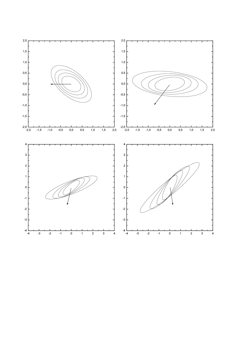
Figure 1: a) (upper left) The projections of the elliptical shells on the plane $(XOY)$ are shown. The origin of the coordinate system is centered at the star’s center of mass, and the plane $(XOY)$ lies in the orbital plane. The spatial scales are expressed in units of the stellar radius $R_{*}$. The ellipses shown correspond to four different Lagrangian coordinates $x=0.2$ (the innermost ellipse), $x=0.4$, $x=0.6$, $x=0.8$. The time $\tau=0$ corresponds to the time of passage of pericenter of the orbit by the star. The arrow is directed toward the hole. b) (upper right) The same as Fig. 1a, but $\tau=1$. c) (bottom left) The same as Fig. 1a, but $\tau=2$. d) (bottom right) The same as Fig. 1a, but $\tau=3$.

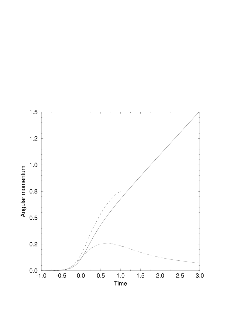
Figure 12: The same as Fig. 10, but $n=3$, $\eta=0.5$. The dashed line is taken from Kh b. Additionally the angular momentum of the gravitationally bounded part of the star is shown (dotted curve).

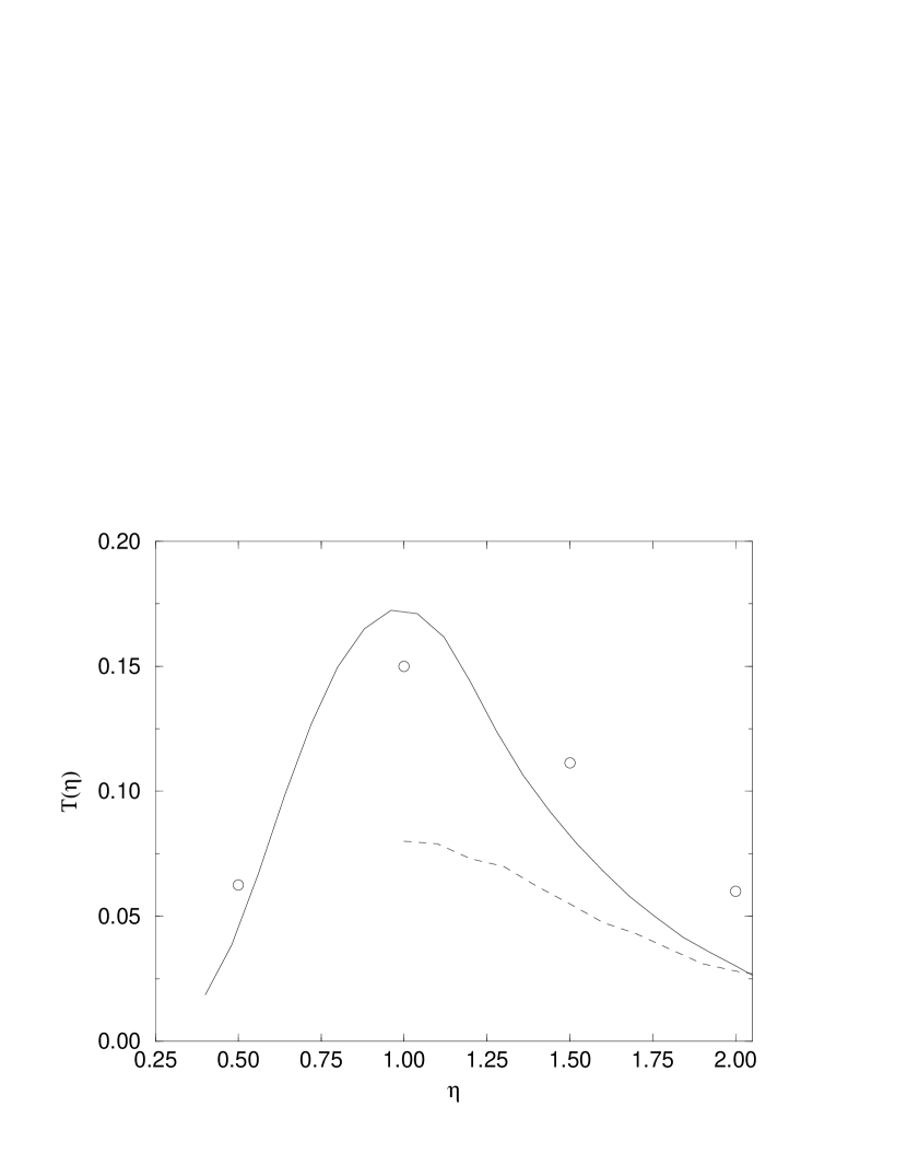
Figure 13: The function $T(\eta)$ is shown for the $n=3$ polytrope. The dashed curve is taken from the paper by Lee $\&$ Ostriker 1986 and corresponds to the analytical linear theory. The open circles show the same quantity calculated by Kh a, b.

The results of our calculations are presented in Figures 1-17.

In Figure 1 (a-d) we show projections of our elliptical shells on the plane $(XOY)$ for four different moments of time $\tau=0$; $1$; $2$; $3$. The shells shown correspond to four different Lagrangian coordinates $x=0.2$; $0.4$; $0.6$; $0.8$. Although the positions of the shells have no direct physical meaning since the shells do not describe directly the mass distribution over the star and can intersect each other, these plots give useful qualitative information about the evolution of our model. The model parameters for these plots $n=1.5$ and $\eta=1.5$ correspond to a tidal encounter of moderate strength. Let us recall that one of the principal axes of the tidal tensor is always oriented toward the black hole, and two others are perpendicular to this direction. Therefore, as we see from Fig.1 (a-d), the principal axes of the shells do not coincide with the principal axes of the tidal tensor, and it can be said that our shells lag behind the changing tidal field. A similar effect has been observed in 3D numerical simulations of the tidal encounter. At the moment $\tau=0$ all shells are almost aligned with respect to each other, but during the subsequent evolution this alignment disappears. The outer layers of the star lag more than the inner layers, and at the time $\tau=3$ intersections between the shells are observed. Approximately at the same time in the 3D finite difference and SPH models the star takes a typical $S$-shaped form.

Figures 2-5 show the evolution of the central density $\rho_{c}$ (expressed in units of the central density $\rho_{c0}$ of the unperturbed star) with time for the different parameters of the model. The dashed lines in Figures 2-4 correspond to the results taken from the 3D finite difference simulations of Kh a,b, and the dashed line in Figure 5 corresponds to the result of SPH simulations by Fulbright et al 1995. The model parameters for these Figures are: $n=1.5$, $\eta=3$ for Fig. 2a; $n=2$, $\eta=3$ for Fig. 2b; $n=2$, $\eta=2.5$ for Fig. 2c; $n=2$, $\eta=2$ for Fig. 2d; $n=3$, $\eta=0.5$ for Fig. 3; $n=2$, $\eta=0.1$ for Fig. 4; $n=1.5$, $\eta=5^{-3/2}\approx 0.0894$ for Fig. 5. Figs 2(a-d) correspond to rather weak tidal forces; Fig. 3 presents the case of moderately strong tidal disruption and Figs 4,5 present the case of a very strong tidal disruption event. For the cases of weak tidal influence we observe oscillations of the star after the moment $\tau=0$. The period of these oscillations is close to the period $T_{f}$ of the fundamental mode of radial stellar pulsations: $T_{f}=3.81$ for $n=1.5$, and $T_{f}=\pi$ for $n=2$ (e.g. Cox 1980). It seems that in our model the amplitude of these oscillations is always smaller than in the 3D simulations. We checked that this decrease of the amplitude does not depend on the value of artificial viscosity used in the computations. Fig. 3 gives an example of a moderately strong tidal disruption event (only about 10 percent of the mass remains gravitationally bounded after this encounter, see Kh b and Figure 17). After $\tau=0$ the central density monotonically decreases with time toward a very small number (we obtained $\rho_{c}/\rho_{c0}\approx 1.4\cdot 10^{-2}$ at the end of our calculations $\tau_{end}=15$). In general our curve is close to the curve obtained in the 3D simulations, but there is a significant deviation near the time $\tau\sim 1$. Unfortunately, the curve obtained in the 3D case is not continued after $\tau=1$, and we cannot say whether our asymptotic value for $\rho_{c}/\rho_{c0}$ is close to the 3D result or not. During the tidal disruption events corresponding to the results presented in Figs 4,5 a very strong tidal disruption of the star occurs, and a typical ’spike’ in the curves for the evolution of the central density is observed. The presence of this ’spike’ has been predicted analytically by Carter $\&$ Luminet $1982$. The amplitude of this ’spike’ is 0.64 times smaller than was obtained by Kh b for the $n=2$, $\eta=0.1$ case, and about $1.6$ times larger than was obtained by Fulbright et al 1995 in their SPH simulations of $n=1.5$, $\eta=0.0894$ case. The asymptotic values of $\rho_{c}/\rho_{c0}$ at the limit of large time almost coincide between our curves and the curves obtained by other methods.

In Figures 6-9 the dependence of total, potential, thermal and kinetic energies on time is shown. In all cases we plot the difference between the energy of a particular kind and its corresponding equilibrium value; $E_{tot}$, $E_{g}$, $E_{th}$ and $E_{K}$ stand for the differences of total, gravitational, thermal and kinetic energies, respectively. We found that too much energy is stored in the outer layers of the star in our model, and calculated the energy differences using $97.5$ percent of the star’s mass . The cases shown are: $n=1.5$, $\eta=3$ (Fig. 6); $n=3$, $\eta=1.5$ (Fig. 7); $n=3$, $\eta=1$ (Fig. 8) and $n=3$, $\eta=0.5$ (Fig. 9). Fig. 6 and Fig. 7 correspond to the case of a small tidal influence on the star, and Figure 8 presents the case of the tidal encounter of a moderate strength. As in the density plots we see the oscillations of the potential and thermal energies, and these oscillations are more pronounced in the 3D simulations (dashed lines). The oscillations of the potential and the thermal energies seem to compensate each other, and there is no oscillation of the total and kinetic energies. The relative difference between the asymptotic (at large time) values of $E_{tot}$ in our calculation and in the 3D calculations is about $10$ percent for the $n=1.5$, $\eta=3$ case, $25$ percent for the $n=3$, $\eta=1.5$ case. The same difference looks small for the case $n=3$, $\eta=1$ (about $7$ percent), but the 3D simulations end at the time $\tau\approx 3.5$ which is too short to make conclusions about the asymptotic value of the total energy. Figure 9 presents the case of a strong tidal encounter. The relative difference of the total energy $E_{tot}$ is about $20$ percent for that case, but again the 3D simulations end at time $\tau\approx 1$ and the asymptotic values of $E_{tot}$ cannot be compared. We see that $E_{tot}$ and $E_{K}$ continue to grow all the time in that case, but this growth takes place only for the gas stripped from the star. Let us define the gravitationally bound debris of the star as a combination of all stars elements where the sum of kinetic and potential energies is less than zero. The dotted line in Figure 9 presents the difference between the total energy of the gravitationally bounded debris and the total energy of the unperturbed star. This difference should tend to an asymptotic value at the large time limit, which is equal to $0.718$ for that case.

Figures 10-12 show the value of angular momentum in the direction perpendicular to the star’s orbit, gained by the star during the tidal encounters. The shown cases are: $n=1.5$, $\eta=3$ (Fig. 10); $n=3$, $\eta=1.5$ (Fig. 11); $n=3$, $\eta=0.5$ (Fig 12). For the cases of weak tidal influence the relative deviation between our model and the 3D results is about $10-20$ percent. For the case of strong tidal disruption the same difference is approximately $10$ percent. In that case the total angular momentum grows with time, but the angular momentum of the gravitationally bound debris tends to a small asymptotic value (the dotted line in Figure 12).

Now we would like to discuss the dependence of the main characteristics of a star after a tidal encounter on the parameter $\eta$ and the polytropic index $n$. For that we should introduce some quantities describing the perturbed star which are conserved when the star leaves the region of effective action of the tidal forces ($\tau\rightarrow\infty$). One such quantity is the difference between the total energy of the gravitationally bounded debris of the star and the total energy of the unperturbed star: $E_{tot}^{bn}$. This quantity sharply decreases with increase of the parameter $\eta$, and therefore it is convenient to introduce another quantity $T(\eta)=\eta^{4}E_{tot}^{bn}$. $T(\eta)$ can be easily compared with results of linear theory of tidal perturbations of a star (Press $\&$ Teukolsky 1977, Lee $\&$ Ostriker 1986), and with results of 3D simulations. We show the result of calculations of this quantity in Figures 13 for a polytropic star with $n=3$, in Figure 14 for the case $n=2$, and in Figure 15 for the case $n=1.5$, respectively . One can see that the difference between the linear theory and our model is small if $\eta$ is rather large ($\eta\sim 2$ for the $n=3$ case, and $\sim 3.5-4$ for the $n=2$, $1.5$ cases), but the linear theory underestimates significantly the energy gain at intermediate values of $\eta$ ($\eta\sim 1,\sim 1.5,\sim 2$ for the $n=3$, $2$, $1.5$ cases respectively). This fact is confirmed by the 3D simulations (open circles in Figures 13-15), and is very transparent from a qualitative point of view. Indeed, the action of tidal forces on the star causes an increase of a characteristic size of the star. In turn, this increase leads to an increase of the characteristic amplitude of the tidal forces. Since the $n=3$ polytrope is more concentrated toward the stellar center of mass than the $n=2$ case, and the $n=2$ polytrope is more concentrated than the $n=1.5$ case, for a given $\eta$ the energy gain of the $n=3$ polytrope is always smaller than the energy gain of the $n=2$, and the energy gain of the $n=2$ polytrope is respectively smaller than the energy gain of the $n=1.5$ case. Note, that the results corresponding to large values of $\eta$ should be taken with care. At first our model may not give exactly the same results as the linear theory in the limit of small tidal perturbations. Second in our numerical model the difference between the numerical value of the total energy for an unperturbed star and its theoretical value is of the order of $10^{-2}$, and this difference is larger than the energy gain corresponding to large values of $\eta$ (e.g $\eta\geq 2$ for the $n=3$ case). Also the circle corresponding to $\eta=0.5$ is shown for illustrative purposes only. For those values of $\eta$ a significant stripping of the star occurs (see Figure 17), and a deviation of the total energy of the star (shown by the circle) and the total energy of the gravitationally bound debris can be significant. In Figure 14 the open circles almost coincide with our curve except for the circle corresponding to $\eta=1.5$, where the difference is rather large (about 40 percent). Perhaps this difference is related to effect of the partial mass stripping of the star, which is rather pronounced for that case. This effect makes the determination of energy of the gravitationally bound debris rather ambiguous, since the gas leaves the star with almost parabolic velocities for this tidal encounter of a moderate strength.

In Figures 16 we show the values of the angular momentum perpendicular to the star’s orbit (taken at the end of calculations $\tau_{end}=10$) and for the gravitationally bound debris (the dotted line) versus $\eta$ for the $n=3$ polytrope. The open circles correspond to the 3D simulations and the dashed curve represents the same quantity calculated by Diener et al 1995 in the framework of the affine model. It seems that in our model the star gets more angular momentum than in the affine model.

In general Figures 13-16 show very good agreement between our results and the results of the 3D simulations. Unfortunately the number of the 3D experiments is too small to make a robust quantitative comparison.

In Figure 17 we show the amount of mass lost by the star after a fly-by around the black hole as a function of $\eta$. Contrary to a ’naive’ Roche-like criterion of tidal disruption (the discussion after eq. 34) we see that there is a partial stripping of mass from the star for a particular range of $\eta$. For the $n=3$ polytrope (the solid line) the star loses its mass if $\eta<\eta_{strip}\approx 1.5$, and the star is completely disrupted if $\eta<\eta_{crit}\approx 0.4$. For the $n=2$ polytrope (the dashed line) we have $\eta_{strip}\approx 2$ and $\eta_{crit}\approx 0.9$ and for the $n=1.5$ polytrope (the dotted line) we have $\eta_{strip}\approx 2.5$ and $\eta_{crit}\approx 1.14$. The values of $\eta_{strip}$ and $\eta_{crit}$ are in excellent agreement with estimates based on the 3D simulations (see Kh b). It is instructive to compare these results with a criterion of tidal disruption obtained in the affine model. In this model Diener et al found that the star is disrupted if $\eta<\eta^{a}_{crit}=0.844$ for $n=3$, $\eta<\eta^{a}_{crit}=1.482$ for $n=2$, $\eta<\eta^{a}_{crit}=1.839$ for $n=1.5$. Since in the affine model the velocity field is self-similar, in this model a partial stripping of outer layers of the star cannot occur. It can be observed that the inequalities $\eta_{crit}<\eta^{a}_{crit}<\eta_{strip}$ always hold, and the difference between the values of $\eta_{crit}^{a}$ and values $\eta_{crit}$ is about 40-50 percent. This difference is much larger than the difference between our values and the results of the 3D calculations. This demonstrates the advantage of our model.

4 Conclusions and Discussion

We have constructed a new model of a star perturbed by a tidal field. In this model the star consists of a set of elliptical shells which in general have different principal axes and different orientations with respect to a fixed locally inertial reference frame comoving with the star’s center of mass. The model obeys certain evolution equations. The results of calculations of a simple problem of tidal encounter of a polytropic star moving on a parabolic orbit around a source of Newtonian gravity have been compared with the results of three dimensional finite difference simulations. We found that the main characteristics of the tidal encounter agree with the results of the finite difference approach with a typical accuracy $10-20$ percent. Taking into account that the astrophysical applications do not demand very high accuracy in description of a single tidal encounter, we think that our model could be used in order to investigate all possible variants of the problem of tidal interaction between a supermassive black hole and a star interesting from an astrophysical point of view. The main advantage of our model is its effectively one dimensional character, which allows us to calculate all interesting variables much faster than the 3D approach, and over a much longer time of evolution. Also, all characteristics of the tidally perturbed star could be inferred from our model in a straightforward and unambiguous way. Our model could also be used in a study of a rotating single star, or a binary star.

In principal, the agreement between our model and 3D computations could be improved if one uses more advanced variants of our model (see below). However we would like to note that in order to make a comparison between an advanced variant of our model and 3D computations, one should also increase both the number of the numerical experiments and their resolution. For example, recently it has been claimed (Ayal et al, 2000) that the difference between the different numerical experiments in SPH models is about 10 percent depending on number of particles used in the calculations. We are not aware of similar convergence studies for the 3D finite difference models. We think that such studies should be undertaken parallel to work on improvement of our model.

Now we would like to discuss possible extensions of our formalism. One obvious way for such extension consists in using a more complicated stellar model for the unperturbed state. Then the realistic stellar models could be generalized to our problem by using the energy evolution equation and the virial relations similar to the eq. (8,9), but written for a realistic stellar gas, with possible inclusion of e.g. non-adiabatic effects, viscosity, effects of radiative transfer, and generation of heat due to nuclear reactions in the stellar core. The evolution equations for such a model could be derived from the energy equation and the virial relations in the way described above. One could also use a more refined numerical scheme, say an implicit scheme with a nonuniform grid. We suppose that certain powerful methods developed in numerical investigations of pulsating stars could be directly applied to our problem. Another interesting extension consists in using the real distribution of the pressure and the density over the volume of the star in our approximation. Thus it is possible to construct a model with no intersection between the shells, which could provide more information about displacements of particular elements of the star during the tidal encounter. Assuming that the star consists of an ideal gas with constant ratio of specific heats $\gamma$, and neglecting the possible presence of shocks in the system, this problem is reduced to the evaluation of the following integrals:

$$I_{1}=\int_{S}R^{2(\gamma-1)}d\Omega,$$

and

$$I_{2i}=\int_{S}l^{2}_{(i)}R^{2\gamma}d\Omega,$$

where the integration is performed over the surface of an ellipsoid $\sum\lambda_{(i)}y^{2}_{(i)}=1$. $\lambda_{i}>0$ are the eigenvalues of the matrix $R^{ln}$ (see. eq. 4), $R$ is the value of the radius vector joining the center of the ellipsoid to a point on its surface, $l_{i}$ are the direction cosines of the radius vector, and $d\Omega$ is the elementary solid angle. The Cartesian coordinates $y_{i}$ are associated with the frame of eigenvectors of the matrix $R^{ln}$. If $\gamma=1$ the integral (35) is trivial, and the integrals (36) are related to the integrals $D_{i}$ defined above (eq. 18), but with $\lambda_{j}^{-1}$ playing the role of $a_{j}^{2}$. One can see that the pressure tensor (defined as the left hand side of the eq. 13) can be evaluated with help of the integrals (35, 36). The volume part of the pressure tensor (the first term on l.h.s. of the eq. (13)) is obtained by integration over the mass of a quantity proportional to the integral (35) with the upper limit of integration determined by some given Lagrangian coordinate $x_{*}$. The surface term ( the second term on l.h.s. of the eq. (13)) is expressed with help of the integrals (36) with $\lambda_{i}=\lambda_{i}(x_{*})$. Note that now the surface term is not symmetric, and therefore transfer of angular momentum between the neighboring shells due to pressure is allowed. If some shells are close to intersection, the density at some particular value of $x$ tends to infinity. That means that some eigenvalues $\lambda_{i}$ go to zero, and as a consequence the integrals (35), (36) tend to infinity causing an increase of pressure. In turn the increase of pressure could prevent the shells from intersecting. The integrals (35), (36) can be evaluated e.g. by numerical means, and serve as main building blocks of a model without intersections between the shells corresponding to different Lagrangian radii.

Finally one can generalize our model to the case of a relativistic tidal field. In a separate paper we apply our model to the problem of tidal interaction of a star with a supermassive Kerr black hole.

Appendix A Reduction of the dynamical equations to the equations of the affine model and the case of an incompressible fluid

Let us consider the position matrix of a special form:

$${\bf T}(t,r_{0})=\hat{\bf T}(t)r_{0},$$

and introduce the matrices $\hat{\bf A}(t)$, $\hat{\bf E}(t)$, $\hat{\bf S}(t)$, and the quantities $\hat{a}_{i}(t)$ defined with the help of the matrix $\hat{\bf T}(t)$ by analogy with the matrices ${\bf A}$, ${\bf E}$, ${\bf S}$, and the quantities $a_{i}$, respectively. For the position matrix of the form (A1) the matrix $R^{ln}$ is:

$$R^{ln}={\delta^{ln}\over r_{0}},$$

and the Jacobian $D=\hat{g}(t)\equiv\hat{a}_{1}\hat{a}_{2}\hat{a}_{3}$ does not depend on the spatial coordinate. Therefore in this case there is no difference between the exact and the averaged values of the density and the pressure. Substituting the expression (A1) into the equations (23), multiplying the result on $r_{0}$ and integrating over $M$, we obtain

$$\ddot{\hat{T}^{i}_{n}}={\Pi\over M_{*}}\hat{S}^{n}_{i}+{\Omega_{*}\over 2M_{*}}{\hat{g}}^{-1}\hat{A}^{i}_{j}\hat{a}_{j}\hat{D}_{j}\hat{E}^{j}_{n}+C^{i}_{j}\hat{T}^{j}_{n},$$

where $\Pi=\int dM{P\over\rho}$, the constant factor $M_{*}={1\over 3}\int dMr_{0}^{2}$ is the scalar quadrupole moment of the star in the unperturbed state and the constant factor $\Omega_{*}=-G\int{MdM\over r_{0}}$ is the self-gravitational energy value in the unperturbed state. The quantities $\tilde{D}_{j}$ are defined with the help of the quantities $\tilde{a}_{j}$ by analogy with the quantities $D_{j}$. The equations (A2) are just the dynamical equations of the affine model (e.g. Carter $\&$ Luminet 1983, 1985 and Luminet $\&$ Carter, 1986).

Now let us consider the case of an incompressible fluid. In this case the density $\rho$ is not changing durind the motion and therefore the constraint $\hat{g}=1$ must be imposed, see eq (6). Assuming that the density is also constant over the whole volume of the star $\rho=\rho_{0}$=const, the equations (A3) can be reduced to a very simple form. Taking into account the constraint $\hat{g}=1$, and performing the integration over $M$ in the expressions for $\Pi$, $M_{*}$, and $\Omega_{*}$, we have

$$\ddot{\hat{T}^{i}_{n}}={\hat{S}^{n}_{i}P_{c}(t)\over 2\rho_{0}R_{*}^{2}}-2\pi G\rho_{0}\hat{A}^{i}_{j}\hat{a}_{j}\hat{D}_{j}\hat{E}^{j}_{n}+C^{i}_{j}\hat{T}^{j}_{n},$$

where $R_{*}$ is the radius of the star and $P_{c}(t)$ is the pressure in the center of the star. Together with the constraint $\hat{g}=1$ the equations (A4) form a complete set of equations. These equations have already been obtained by Luminet and Carter (see eq. (3.1a) in Luminet $\&$ Carter, 1986) . It has been proved that the equations (A4) follow from the hydrodynamical equations without any approximation.

Appendix B The numerical scheme

For our numerical work it is convenient to introduce the potential energy tensor density per unit of mass:

$$F^{ik}={d\over dM}\bar{\cal P}^{ik}=-{1\over 2}GMA^{i}_{l}A^{k}_{l}{a^{2}_{l}D_{l}\over g},$$

and use dimensionless representations of all variables. We use the dimensionless mass coordinate $x=M/M_{*}$, and the dimensionless time $\tau=\sqrt{{GM_{*}\over R_{*}^{3}}}t$. $\Delta x$ stands for the mass coordinate step, and $\Delta\tau$ stands for the time step. The dimensionless dynamical variables are defined as follows:

$$\tilde{\bf T}={\bf T}/R_{*},\quad\tilde{\bf V}={\partial\over\partial\tau}\tilde{\bf T},$$

$$\tilde{\bf F}={R_{*}\over GM_{*}}{\bf F},$$

$$\tilde{g}=g/R_{*}^{3},\quad\tilde{\rho}={4\pi R_{*}^{3}\over 3M_{*}}\rho,$$

$$\tilde{P}={4\pi R^{4}_{*}\over GM_{*}^{2}}P,\quad\tilde{\epsilon}={\tilde{P}\over(\gamma-1)},$$

the dimensionless tidal tensor is

$$\tilde{\bf C}={R_{*}^{3}\over GM_{*}}\bf C.$$

We use a uniform grid along the mass coordinate with number of the grid points $J=201$ (the first and the last numbers correspond respectively to the center of the star, and to the star’s boundary). The pressure, the density and the energy density are defined at the centers of zones between the grid points, and are denoted by the indices $j+1/2$, $j-1/2$, and the position matrix and its time derivative are defined at the grid points. Hereafter the index $n$ denotes a time level, and the index $j$ denotes a particular grid point, and no summation over those indices is assumed.

We use several intermediate steps to advance our model from $\tau^{n}$ to $\tau^{n+1}$. First we calculate $\tilde{\bf C}$, and $\tilde{g}^{n}_{j}$ and $\tilde{\bf F}^{n}_{j}$ with help of special subroutines. To calculate the rotational matrix ${\bf A}$ and the principal axes $a_{l}$ we use the standard Jacobi method. Then we calculate the dimensionless expansion rate

$$\tilde{H}^{n}_{j}={1\over 3}(\tilde{\bf S}\cdot\tilde{\bf T})^{n}_{j},$$

where $\cdot$ stands for the contraction over all indices, and the density

$$\tilde{\rho}^{n}_{j-1/2}={\Delta x\over(\tilde{g}^{n}_{j}-\tilde{g}^{n}_{j-1})},$$

Next the artificial (bulk) viscosity term is calculated according to the rule:

$$v^{n}_{j}=(\tilde{H}{\tilde{g}}^{1/3})^{n}_{j},\quad q^{n}_{j-1/2}=b^{2}\tilde{\rho}^{n}_{j-1/2}{(\Delta x)}^{2}{(v^{n}_{j}-v^{n}_{j-1})}^{2},$$

if $v^{n}_{j}-v^{n}_{j-1}<0$, and

$$q^{n}_{j-1/2}=0,$$

if $v^{n}_{j}-v^{n}_{j-1}>0$. The artificial viscosity is very useful in the calculations, since it dampen the small scale (unphysical) modes. We used $b=2$ in our calculations, and checked that smaller values of $b$ lead to the same motion, but with additional small scale oscillations of the dynamical variables. After calculation of all these variables we advance the position matrix and its time derivative to the next time level:

$$\tilde{\bf v}^{n+1}_{j}=\tilde{\bf v}^{n}_{j}+\Delta\tau(-(\tilde{\bf S}^{T}\tilde{g})^{n}_{j}{\partial\tilde{P}\over\partial x}+3{(\tilde{\bf S}^{T}\tilde{\bf F})}^{n}_{j}+{(\tilde{\bf C}\tilde{\bf T})}^{n}_{j}),$$

where

$${\partial\tilde{P}\over\partial x}={(\tilde{P}^{n}_{j+1/2}+q^{n}_{j+1/2}-\tilde{P}^{n}_{j-1/2}-q^{n}_{j-1/2})\over\Delta x},$$

and

$$\tilde{T}^{n+1}_{j}=\tilde{T}^{n}_{j}+\Delta\tau\tilde{\bf v}^{n+1}_{j}.$$

Note, that the scheme (B10-B11) conserves the circulation, and it also conserves the angular momentum provided the tidal term is ’switched off’. To calculate the change of the energy density and the pressure, we calculate the kinetic energy term ${\dot{\bf T}\cdot\dot{\bf T}^{T}\over 2}$, and the potential energy term $tr({\bf F})$ for the both time levels, and also the density $\tilde{\rho}^{n}_{j-1/2}$ for the $n+1$ time level. Then we have

$$\tilde{\epsilon}^{n+1}_{j-1/2}=\tilde{\rho}^{n+1}_{j-1/2}({\tilde{\epsilon}^{n}_{j-1/2}\over\tilde{\rho}^{n}_{j-1/2}}-(\Delta E_{k}+\Delta E_{p})+\Delta\tau Q),$$

where

$$\Delta E_{k}={({\dot{\bf T}\cdot\dot{\bf T}^{T}\over 2})}^{n+1}_{j}-{({\dot{\bf T}\cdot\dot{\bf T}^{T}\over 2})}^{n}_{j}\quad\Delta E_{p}=3tr({\bf F}^{n+1}_{j}-{\bf F}^{n}_{j}),$$

and

$$Q=-3{(\tilde{H}^{n}_{j}\tilde{g}^{n}_{j}(\tilde{P}^{n}_{j+1/2}+q^{n}_{j+1/2})-\tilde{H}^{n}_{j-1}\tilde{g}^{n}_{j-1}(\tilde{P}^{n}_{j-1/2}+q^{n}_{j-1/2}))\over\Delta x}+{(\tilde{\bf C}\tilde{\bf T}\cdot\tilde{\bf V}^{T})}^{n}_{j}.$$

The eq. (B12) tells that the scheme is conservative with respect to the law of energy conservation.

The boundary conditions for our problem are

$${\bf T}^{n}_{1}={\bf V}^{n}_{1}=0,\quad\tilde{\rho}^{n}_{1/2}=\tilde{\rho}^{n}_{3/2},$$

and

$$\tilde{P}^{n}_{J}=0.$$

The initial static stellar configurations are calculated by a shooting method described by e.g. Khokhlov 1991.

The size of the time step must follow from the stability analysis of our scheme, which is rather complicated. Therefore we constrain our time step by the condition:

$$\Delta\tau={\alpha\Delta x\over c_{s}},$$

where

$$c_{s}={\Delta x\over{\tilde{g}\sqrt{\gamma(\tilde{P}+q)\tilde{\rho}(\tilde{\bf S}\cdot\tilde{\bf S}^{T})}}},$$

is the velocity of propagation of a small perturbation (with respect to the mass coordinate) calculated in analytical linear approximation, and $\alpha$ is a parameter. We used $\alpha=1/15$ for all our calculations except the case $n=2$, $\eta=0.1$, where $\alpha=1/60$ has been used, and the case $n=1.5$, $\eta=0.0894$, where we used $\alpha=1/120$. In the case of the evolution of a pulsating star our condition (B17) is reduced to the well known von Neumann-Richtmyer condition provided $\alpha=1/\sqrt{(4\pi)}$ (e.g Richtmyer $\&$ Morton, 1967, p. 297-298).

We tested our scheme against Sedov’s analytical solution for a motion of an expanding spherical gas cloud, and also the problem of small oscillations in a polytropic star. In the both cases we found very good agreement between the analytical theory and our scheme.

Figure 2: a) (upper left) The evolution of the central density (expressed in units of the central density of the unperturbed star) is shown as a function of time. The parameters of tidal encounter are $n=1.5$, $\eta=3$. The solid curve is calculated from our model, and the dashed curve is calculated in 3D simulations of Kh a. b) (upper right) The same as Fig. 2a, but $n=2$, $\eta=3$. c) (bottom left) The same as Fig. 2a, but $n=2$, $\eta=2.5$. d) (bottom right) The same as Fig. 2a, but $n=2$, $\eta=2$.

Figure 3: The evolution of the central density in case of a strong tidal encounter. The dashed curve corresponds to the simulations of Kh b. The parameters are $n=3$, $\eta=0.5$.

Figure 4: The ’spike’ in the evolution curve of the central density due to very strong tidal encounter, the dashed curve corresponds to the simulations of Kh b. The parameters are $n=3$, $\eta=0.1$.

Figure 5: The same as Fig. 4, but $n=1.5$, $\eta=0.0894$. The dashed curve is calculated in SPH simulations of Fulbright et al, 1995.

Figure 6: The evolution of the total $E_{tot}$, thermal $E_{th}$ and gravitational $E_{g}$ energies with time. All sorts of energy are measured with respect to their equilibrium values. The solid curves correspond to our model, and the dashed curves correspond to the simulations of Kh a. The case $n=1.5$, $\eta=3$ is shown.

Figure 7: The same as Fig. 6, but $n=3$, $\eta=1.5$. Additionally the evolution of the kinetic energy $E_{K}$ is shown.

Figure 8: The same as Fig. 7, but $n=3$, $\eta=1$.

Figure 9: The same as Fig. 7, but $n=3$, $\eta=0.5$. The dashed curves are taken from Kh b. Additionally the total energy of the gravitationally bounded part of the star is shown (dotted curve).

Figure 10: The evolution of $z$ component of angular momentum with time. The dashed line is taken from Kh a. The case $n=1.5$, $\eta=3$ is shown.

Figure 11: The same as Fig. 10, but $n=3$, $\eta=1.5$.

Figure 14: The same as Fig. 13, but for $n=2$ polytrope.

Figure 15: The same as Fig. 13, but for $n=1.5$ polytrope.

Figure 16: The dependence of the angular momentum gained by the star at the end of calculations ($\tau_{end}=10$) on the parameter $\eta$. The solid curve represents the total angular momentum, the dotted line represents the angular momentum of the gravitationally bounded part of the star. The dashed curve represents the same quantity calculated in the affine model by Diener et al 1995, and the open circles correspond to the simulations of Kh a, b. The case of $n=3$ polytrope is shown.

Figure 17: The amount of mass lost by the star in course of tidal encounters. The solid curve corresponds to the $n=3$ polytrope, the dashed curve corresponds to the $n=2$ polytrope and the dotted curve corresponds to the $n=1.5$ polytrope.

References

- Aurière (1982) Ayal, S., Livio, M Piran, T. 2000, astro-ph/0002499
- Canizares et al. (1978) Beloborodov, A. M., Illarionov, A. F., Ivanov, P. B. Polnarev, A. G. 1992, MNRAS, 259, 209
- Djorgovski and King (1984) Bicknell, G. V. Gingold, R. A. 1983, ApJ, 273, 749
- Hagiwara and Zeppenfeld (1986) Cannizzo, J. K., Lee, H. M. Goodman, J. 1990, ApJ, 351, 38
- Harris and van den Bergh (1984) Carter, B. Luminet, J. P. 1982, Nature, 296, 211
- Hènon (1961) Carter, B. Luminet, J.-P. 1983, A&A, 121, 97
- King (1966) Carter, B. Luminet, J.-P. 1985, MNRAS, 212, 23
- King (1975) Chandrasekhar, S. 1969, ”Ellipsoidal Figures of Equilibrium”, New Haven and London, Yale University Press
- King (1975) Cox, J. P. 1980 ”Theory of stellar pulsation”, Princeton, New Jersey, Princeton University Press
- King et al. (1968) Diener, P., Kosovichev, A. G., Kotok, E. V., Novikov, I. D. Pethick, C. J. 1995, MNRAS, 275, 498
- Kron et al. (1984) Diener, P., Frolov, V. P., Khokhlov, A. M., Novikov, I. D., Pethick, C. J. 1997 ApJ, 479, 164
- Lynden-Bell and Wood (1968) Dokuchaev, V. I. 1991, MNRAS, 251, 564
- Newell and O’Neil (1978) Evans, C. R. Kochanek, C. S 1989, ApJ, 346L, 13
- Ortolani et al. (1985) Fishbone, L. 1973, ApJ, 185, 43
- Peterson (1976) Frank, J. Rees, M. J. 1976, MNRAS, 176, 633
- Spitzer (1985) Frank, J. 1979, MNRAS, 187, 883
- Spitzer (1985) Frolov, V. P., Khokhlov, A. M., Novikov, I. D. Pethick, C. J. 1994, ApJ, 432, 680
- Spitzer (1985) Fulbright, M. S., Benz, W. Davies, M. B 1995, ApJ, 440, 254
- Spitzer (1985) Gurzadian, V. G. Ozernoi, L. M., 1980, A&A, 86, 315
- Spitzer (1985) Hills, J. G. 1975, Nature, 254, 295
- Spitzer (1985) Hills, J. G. 1978, MNRAS, 182, 517
- Spitzer (1985) Illarionov, A. F. Romanova, M. A., 1986a, Soviet Astr., 32, 148
- Spitzer (1985) Illarionov, A. F. Romanova, M. A., 1986b, Soviet Astr., 32, 356
- Spitzer (1985) Khokhlov, A. M. 1991, A&A, 245, 114
- Spitzer (1985) Khokhlov, A., Novikov, I., D. Pethick, C. J. 1993a, ApJ, 418, 163
- Spitzer (1985) Khokhlov, A. M., Novikov, I. D. Pethick, C. J. 1993b, ApJ, 418, 181
- Spitzer (1985) Kim, S. S., Park, M.-G., Lee, H. M. 1999, ApJ, 519, 647
- Spitzer (1985) Kochanek, C., S. 1994, ApJ, 423, 344
- Spitzer (1985) Kosovichev, A. G. Novikov, I. D. 1992, MNRAS, 258, 715
- Spitzer (1985) Lacy,J. H., Townes, C. H. Hollenbach, D. J. 1982, ApJ, 262, 120
- Spitzer (1985) Laguna, P., Miller, W. A., Zurek, W. H. Davies, M. B. 1993, ApJ, 410L, 83
- Spitzer (1985) Laguna, P. 1994, ApJ, 404, 678
- Spitzer (1985) Lai, D., Rasio, F., A. Shapiro, S., L. 1994, ApJ, 437, 742
- Spitzer (1985) Lai, D. Shapiro, S., L. 1995, MNRAS, 275, 498
- Spitzer (1985) Lattimer, J. M. Schramm, D. N. 1976 ApJ, 210, 549
- Spitzer (1985) Lee, H. M., Ostriker, J. P. 1986, ApJ, 310, 176
- Spitzer (1985) Luminet, J.-P. Pichon, B. 1989, A&A, 209, 103
- Spitzer (1985) Luminet, J.-P. Carter, B. 1986, ApJS, 61, 219
- Spitzer (1985) Luminet, J.-P. Mark, J.-A. 1985, MNRAS, 212, 57
- Spitzer (1985) Magorrian, J. Tremaine, S. 1999, MNRAS, 309, 477
- Spitzer (1985) Mark, J.-A., Lioure, A. Bonazzola, S. 1996, A&A, 306, 666
- Spitzer (1985) Mashhoon, B. 1975, ApJ, 197, 705
- Spitzer (1985) Nduka, A. 1971, ApJ170, 131
- Spitzer (1985) Nolthenius, R. A. Katz, J. I. 1983, ApJ, 269, 297
- Spitzer (1985) Novikov, I. D., Pethick, C. J. Polnarev, A. G. 1992, MNRAS, 255, 276
- Spitzer (1985) Press, W. H., Teukolsky, S. A. 1977, ApJ, 213, 183
- Spitzer (1985) Rees, M. J., 1988, Nature, 333, 523
- Spitzer (1985) Roos, N. 1992, ApJ, 385, 108
- Spitzer (1985) Richtmyer, R. D Morton, K. W. 1967, “Difference Methods for Initial-Value Problems”. Second Edition. New York/ London, Interscience Publishers
- Spitzer (1985) Syer, D Ulmer, A. 1999, MNRAS, 306, 35
- Spitzer (1985) Ulmer, A. 1999, ApJ, 514, 180
- Spitzer (1985) Ulmer, A., Paczynski, B. Goodman, J. 1998, A&A, 333, 379
- Spitzer (1985) Young, P. J., Shields, G. A. Wheeler, J. C. 1977, ApJ, 212, 367
- Spitzer (1985) Young, P. J. 1977, ApJ, 215, 36