May 3, 2000 OAT Int. Rep. 71/00 OAT Pub. Num. 2140 Submitted to PASP
Data Streams from the Low Frequency Instrument
On-Board the Planck Satellite:
Statistical Analysis and Compression Efficiency

Abstract

The expected data rate produced by the Low Frequency Instrument (LFI) planned to fly on the ESA Planck mission in 2007, is over a factor 8 larger than the bandwidth allowed by the spacecraft transmission system to download the LFI data. We discuss the application of lossless compression to Planck/LFI data streams in order to reduce the overall data flow. We perform both theoretical analysis and experimental tests using realistically simulated data streams in order to fix the statistical properties of the signal and the maximal compression rate allowed by several lossless compression algorithms. We studied the influence of signal composition and of acquisition parameters on the compression rate $C_{\mathrm{r}}$ and develop a semiempirical formalism to account for it. The best performing compressor tested up to now is the arithmetic compression of order 1, designed for optimizing the compression of white noise like signals, which allows an overall compression rate $\overline{\mbox{$C_{\mathrm{r}}$}}=2.65\pm 0.02$. We find that such result is not improved by other lossless compressors, being the signal almost white noise dominated. Lossless compression algorithms alone will not solve the bandwidth problem but needs to be combined with other techniques.

1 Introduction and Scanning Strategy

The Planck satellite (formerly COBRAS/SAMBA, Bersanelli et al. (1996)), which is planned to be launched in 2007, will produce full sky CMB maps with high accuracy and resolution over a wide range of frequencies (Mandolesi et al. (1998a); Puget et al. (1998)). Table 1 summarizes the basic properties of LFI aboard Planck. The reported sensitivities per resolution element – i.e. a squared pixel with side equal to the Full Width at Half Maximum (FWHM) extent of the beam –, in terms of antenna temperature, represents the goals of LFI for 14 months of routine scientific operations) as recently revised by the LFI Consortium (Mandolesi et al. (1999)).

The limited bandwidth reserved to the downlink of scientific data calls for huge lossless compression, theoretical upper limit being about four (Maris et al. (1999)). Careful simulations are demanded to quantify the capability of true compressors for “realistic” synthetic data and improve the theoretical analysis, including CMB signal (monopole, dipole and anisotropies), foregrounds and instrumental noise.

During the data acquisition phase the Planck satellite will rotate at a rate of one circle per minute around a given spin axis that changes its direction every hour (of 2.5^′ on the ecliptic plane in the case of simple scanning strategy), thus observing the same circle on the sky for 60 consecutive times (Mandolesi et al. (1998a, b)). LFI will produce continuous data streams of temperature differences between the microwave sky and a set of on-board reference sources; both differential measurements and reference source temperatures must be recorded.

The LFI Proposal assumes a sampling time $\tau_{\mathrm{s}}\sim 7$ msec for each detector (Mandolesi et al. (1998a)), thus calling for a typical data rate of $\sim 260$ Kb/sec, while the allocated bandwidth to download Planck data to ground is in total $\sim 60$ Kb/sec. Assuming the total bandwidth to be equally split between instruments, $\approx 30$ Kb/sec on the average would be assigned to LFI asking for a compression of about a factor $8.4$. Data have to be downloaded without information losses and by minimizing scientific processing on board.

A possible solution would be to adapt the sampling rate to the angular resolution specific for each frequency. This should allow to save about up to a factor $\approx 9$ for the 30 GHz channel, but since only $\approx 7\%$ of the samples come from such channel (see table 1) the overall reduction in the final data rate would be $\approx 17\%$.

On the other hand, it is unlikely that the bandwidth for the downlink channel may be enhanced to solve the bandwidth problem, since the ground facilities are shared between different missions and there is the need to minimize possible cross-talks between the instrument and the communication system.

With the aim of optimizing of the transmission bandwidth dedicated to the downlink of LFI data from the Planck spacecraft to the FIRST/Planck Ground Segment, we analyze in detail the role that can be played by lossless compression of LFI data before they are sent to Earth.

We apply different compression algorithms to suitable sets of Planck LFI simulated data streams generated by considering different combinations of astrophysical and instrumental signals and for different instrumental characteristics and detection electronics.

The first considered contribution is that introduced by receiver noise: we consider here the case of pure white noise and of white noise coupled to $1/f$ noise with different knee frequencies. The reference load temperature is assumed to be 20 K for present tests; because of the strong dependence of the $1/f$ noise on the load temperature, this can be considered a worst case, since the actual baseline reference load is of 4 K.

Different sky signal sources are subsequently added to the receiver noise: CMB fluctuations, CMB dipole, Galaxy emission and extragalactic point sources. The signal from the different sky components are convolved with the corresponding antenna pattern shapes, assumed to be symmetric and gaussian with the FWHM reported in Table 1.

We generate simulated data streams at the two extreme frequency channels, 30 GHz and 100 GHz and consider data streams with different time lengths.

Regarding the detection electronics, we explore different signal offset and scaling.

The large number of above combinations was systematically explored using an automated program generator as described by Maris & Staniszkis (1998).

In Section 2 we characterize quantitatively the LFI signal component by component. Section 3 we discuss how the acquisition chain is modeled to perform compression simulations. A theoretical analysis of the compression efficiency is presented in section 4. While section 5 is devoted to the analysis of the signal statistics. The subject of quantization error is illustrated in section 6. The experimental protocol and results about compression are reported in section 7. Further constraints on the on-board data compression are reported in section 8. A proposal for an alternative coding method is made in section 9. The overall compression rate is estimated in section 10. Conclusions are in section 11. Appendix A is included to further illustrate the estimation of the overall compression rate.

2 Characterization of Planck/LFI signal components

The simulated cosmological and astrophysical components are generated according to the methods described in Burigana et al. (1998b) and the data stream and noise generation as in Burigana et al. (1997b), Seiffert et al. (1997) and Maino et al. (1999). We summarize here below the basic points.

$\bullet$ Modeling the CMB pattern – The CMB monopole and dipole have been generated by using the Lorentz invariance of photon distribution functions, $\eta$, in the phase space (Compton–Getting effect): $\eta_{obs}(\nu_{obs},\vec{n})=\eta_{CMB}(\nu_{CMB})\,$, where $\nu_{obs}$ is the observation frequency, $\nu_{CMB}=\nu_{obs}(1+\vec{\beta}\times\vec{n})/\sqrt{1-\beta^{2}}$ is the corresponding frequency in the CMB rest frame, $\vec{n}$ is the unit vector of the photon propagation direction and $\vec{\beta}=\vec{v}/c$ the observer velocity. A blackbody spectrum at $T_{0}=2.725$ K (Mather et al. (1999)) is assumed for $\eta$. For gaussian models, the CMB anisotropies at $l\geq 2$ can be simulated by following the standard spherical harmonic expansion (see, e.g., Burigana et al. (1998a) or by using FFT (Fast Fourier Transform) techniques which take advantage of equatorial pixelisations (Muciaccia et al. (1997))).

$\bullet$ Modeling the Galaxy emission – The Haslam map at 408 MHz (Haslam et al. (1982)) is the only full-sky map currently available albeit large sky areas are sampled at 1420 MHz (Reich & Reich (1986)) and at 2300 MHz (Jonas et al. (1998)). To clean these maps from free-free emission we use a 2.7 GHz compilation of $\sim$ 7000 HII sources (Witebsky (1978)), private communication) at resolution of $\sim$ 1^∘. They are subtracted for modelling the diffuse components and then re-added to the final maps. We use a spectral index $\beta_{ff}=2.1$ from 2.7 to 1 GHz and $\beta_{ff}=0$ below 1 GHz. We then combine the synchrotron maps producing a spectral index map between 408-2300 MHz with a resolution of $\mbox{$\stackrel{{{}_{<}}}{{{}_{\sim}}}$}2^{\circ}\div 3^{\circ}$ ($<\beta_{sync}>\sim 2.8$). This spectral index map is used to scale the synchrotron component down to $\sim$ 10 GHz. In fact, for typical (local) values of the galactic magnetic field ($\sim 2.5\mu$G), the knee in the electron energy spectrum in cosmic rays ($\sim$ 15 Gev) corresponds to $\sim$ 10 GHz (Platania et al. (1998)). From the synchrotron map obtained at 10 GHz and the DMR 31.5 GHz map we derive a high frequency spectral index map for scaling the synchrotron component up to Planck frequencies. These maps have a poor resolution and the synchrotron structure needs to be extrapolated to Planck angular scales. An estimate of the synchrotron angular power spectrum and of its spectral index, $\gamma$ ($C_{l}\propto l^{-\gamma}$), has been provided by Lasenby et al. (1998); we used $\gamma=3$ for the angular structure extrapolation (Burigana et al. (1998a)). Schlegel (Schlegel et al. (1998)) provided a map of dust emission at 100$\mu$m merging the DIRBE and IRAS results to produce a map with IRAS resolution ($\simeq 7^{\prime}$) but with DIRBE calibration quality. They also provided a map of dust temperature, $T_{d}$, by adopting a modified blackbody emissivity law, $I_{\nu}\propto B_{\nu}(T_{d})\nu^{\alpha}$, with $\alpha=2$. This can be used to scale the dust emission map to Planck frequencies using the dust temperature map as input for the $B_{\nu}(T_{d})$ function. Unfortunately the dust temperature map has a resolution of $\simeq 1^{\circ}$; again, we use an angular power spectrum $C_{l}\propto l^{-3}$ to scale the dust skies to the Planck proper resolution. Merging maps at different frequencies with different instrumental features and potential systematics may introduce some internal inconsistencies. More data on diffuse galactic emission, particularly at low frequency, would be extremely important.

$\bullet$ Modeling the extragalactic source fluctuations – The simulated maps of point sources have been created by an all–sky Poisson distribution of the known populations of extragalactic sources in the $10^{-5}<S(\nu)<10$ Jy flux range exploiting the number counts of Toffolatti et al. (1998) and neglecting the effect of clustering of sources. The number counts have been calculated by adopting the Danese et al. (1987) evolution model of radio selected sources and an average spectral index $\alpha=0$ for compact sources up to $\simeq 200$ GHz and a break to $\alpha=0.7$ at higher frequencies (see Impey & Neugebauer (1988); De Zotti & Toffolatti (1998)), and by the model C of Franceschini et al. (1994) updated as in Burigana et al. (1997a), to account for the isotropic sub-mm component estimated by Puget et al. (1996) and Fixsen et al. (1996). At bright fluxes, far–IR selected sources should dominate the number counts at High Frequency Instrument (HFI) channels for $\nu\mbox{$\stackrel{{{}_{>}}}{{{}_{\sim}}}$}300$ GHz, whereas radio selected sources should dominate at lower frequencies (Toffolatti et al. (1998)).

$\bullet$ Instrumental noise – The white noise depends on instrumental performances (bandwidth $\Delta\nu$, system temperature $T_{sys}$), on the observed sky signal, $T_{sky}$, dominated by CBM monopole, and on the considered integration time, $\tau$, according to:

$$\Delta T_{\rm wn}=\frac{\sqrt{2}(T_{sys}+T_{sky})}{\sqrt{\Delta\nu\,\tau}}\,.$$ (1)

Under certain idealistic assumptions, Burigana et al. (1997b) and Seiffert et al. (1997) provide analytical estimates for the knee frequency, $f_{k}$, of LFI radiometers; it is predicted to critically depend also on the load temperature, $T_{load}$, according to:

$$f_{k}=\frac{A^{2}{\Delta\nu}}{8}(1-r)^{2}\left(\frac{T_{sys}}{T_{sys}+T_{sky}}\right)^{2}\,,$$ (2)

where $r=(T_{sky}+T_{sys})/(T_{load}+T_{sys})$ and $A$ is a constant, depending on the state of art of radiometer technology, which has to be minimized for reducing via hardware the knee frequency (current estimates are $A\sim 1.8\times 10^{-5}$ for 30 and 44 GHz radiometers and $A\sim 2.5\times 10^{-5}$ for 70 and 100 GHz).

Recent experimental results from Seiffert (private communication Seiffert (1999)) show knee frequency values of this order of magnitude, confirming that the present state of art of the radiometer technology is close to reach the ideal case.

A pure white noise stream can be easily generated by employed well tested random generator codes and normalizing their output to the white noise level $\Delta T_{\rm wn}$. A noise stream which takes into account both white noise and $1/f$ noise can be generated by using FFT methods. After generating a realisation of the real and imaginary part of the Fourier coefficients with spectrum defined $S_{noise}(f)\propto(1+f_{k}/f)$, we transform them and obtain a real noise stream which has to be normalized to the white noise level $\Delta T_{\rm wn}$ (Maino et al. (1999)).

$\bullet$ Modeling the observed signal – We produce full sky maps, $T_{sky}$, by adding the antenna temperatures from CMB, Galaxy emission and extragalactic source fluctuations. Planck will perform differential measurements and not absolute temperature observations; we then represent the final observation in a given $i$-$th$ data sample in the form $T_{i}=R_{i}(T_{sky,i}+N_{i}-T_{x,i}^{r})\,$, where $N_{i}$ is the instrumental noise generated as described above.

$T_{x,i}^{r}$ is a reference temperature subtracted in the differential data and $R_{i}$ is a constant which accounts for the calibration. Of course, the uncertainty on $R_{i}$ and the non reduced time variation of $T_{x,i}^{r}$ have to be much smaller than the Planck nominal sensitivity. Thus, we generate the “observed” map assuming a constant value, $T_{x}^{r}$, of $T_{x,i}^{r}$ for all the data samples. We note that possible constant small off-sets in $T_{x}^{r}$ could be in principle accepted, not compromising an accurate knowledge of the anisotropy pattern. We arbitrarily generate the “observed” map with $R_{i}=R=1$ for all the data samples.

3 A model of Acquisition Chain

To test rigorously the efficiency of different compressors the best solution is to generate a realistically simulated signal for different mission hypotheses and apply to them the given compressors. To be realistical the simulation of the signal generation should contain both astrophysical and instrumental effects. It would be helpful that the final simulation would be able to given a hint about the influence of the various signal components and their variance. Of course it is useless to reproduce in full detail the LFI to obtain a signal simulation accurate enough to test compressors. A simplified model of the LFI, its front-end electronics and its operations will be enough.

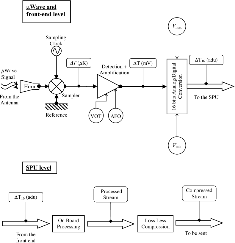
Figure 1: Scheme for the functional model of the acquisition pipeline.

At the base of the simplified model is the concept of acquisition pipeline. This pipeline is composed by all the modules which process the astrophysical signal: from its collection to the production of the final data streams which are compressed and then sent to Earth. In the real LFI, the equivalent of the acquisition pipeline may be obtained following the flow of the astrophysical information, from the telescope through the front-end electronics and the main Signal Processing Unit (SPU) to the memory of the Data Processing Unit (DPU) which is in charge to downlink it to the computer of the spacecraft and then to Earth. The acquisition pipeline is represented in figure 1. Since its purpose is to describe the signal processing and its parameters it must not be regarded as a representation of the true on-board electronics since some functionalities may be shared between different real modules. In this scheme Front End operations of the true LFI are assigned to the first simulation level, while on-board processing and compression to the second one.

The simulated microwave signal from the sky is collected and compared with the temperature of a reference load which, in our simulations, is supposed to have exactly the CMB temperature $T_{0}=2.725$ K (Mather et al. (1999)) . The difference $\Delta T$ expressed in $\mu$K is sampled along a scan circle producing a data stream of 60 scan circles with 8640 samples (pointings).

Signal detection is simulated by Bersanelli et al. (1996); Maris et al. (1998, 1999)

$$\mbox{$V_{\mathrm{out}}$}=\mbox{$\mathrm{AFO}$}+\mbox{${\mathrm{VOT}}$}\cdot\Delta T,$$ (3)

where $V_{\mathrm{out}}$ is the detection chain output in Volts, ${\mathrm{VOT}}$ is the antenna temperature to the detector voltage conversion factor ($-0.5$V/K $\leq VOT\leq+1.5$ V/K) while $\mathrm{AFO}$ is a detection chain offset ($-5$V $\leq\mbox{$\mathrm{AFO}$}\leq+5$V). Of course in our simulation this offset takes into account all offset sources, including variations of the reference temperature, and not only of the electrical offset. Similarly the ${\mathrm{VOT}}$ factor takes into account also differences among the different detectors which affect the calibration of the temperature/voltage relation. The range for ${\mathrm{VOT}}$ and $\mathrm{AFO}$ is large enough to include the whole set of nominal instrumental configurations, allowing also for somewhat larger and smaller values.

The analog to digital conversion (ADC) is described by the formula:

$$\mbox{$V_{\mathrm{out}}^{\mathrm{adu}}$}\mathrm{(adu)}=\mbox{$\mathrm{trunc}$}\left(2^{\mbox{$N_{\mathrm{bits}}$}}\;\cdot\;\frac{\mbox{$V_{\mathrm{out}}$}-\mbox{$V_{\mathrm{min}}$}}{\mbox{$V_{\mathrm{max}}$}-\mbox{$V_{\mathrm{min}}$}}\right),$$ (4)

where $\mbox{$\mathrm{trunc}$}(.)$ is the decimal truncation operator, $N_{\mathrm{bits}}$ is the number of quantization bits produced by the ADC, while $V_{\mathrm{min}}$ and $V_{\mathrm{max}}$ are the lower and upper limits of the voltage scale accepted in input by the ADC. In our case: $\mbox{$N_{\mathrm{bits}}$}=16$ bits, $\mbox{$V_{\mathrm{min}}$}=-10$ V, $\mbox{$V_{\mathrm{max}}$}=+10$ V. So the quantization unit “adu” (analog/digital unit) is

$$1\,\mbox{$\mathrm{adu}$}=\frac{\mbox{$V_{\mathrm{max}}$}-\mbox{$V_{\mathrm{min}}$}}{2^{\mbox{$N_{\mathrm{bits}}$}}}$$ (5)

or in terms of antenna temperature the quantization step is

$$\Delta=\frac{\mbox{$V_{\mathrm{max}}$}-\mbox{$V_{\mathrm{min}}$}}{2^{\mbox{$N_{\mathrm{bits}}$}}\mbox{${\mathrm{VOT}}$}}$$ (6)

for a typical $\mbox{${\mathrm{VOT}}$}=1$ V/K, $\mbox{$N_{\mathrm{bits}}$}=16$ bits, $1\;\Delta\approx 3\times 10^{-4}$ K/adu. After digitization the simulated signal is written into a binary file of 16 bits integers and sent to the compression pipeline.

The simplified LFI is composed of four acquisition pipelines, one for each frequency, each one being representative of the set of devices which form the full detection channel for the given frequency. The overall data-rate after loss-less compression for LFI should be obtained summing the contribution expected from each detector. Since in the real device each radiometer for a given frequency channel, will be characterized by different values of ${\mathrm{VOT}}$ and $\mathrm{AFO}$, the distribution of these parameters has to be taken in account computing the overall compression efficiency. In particular a greater attention should be devoted to the distribution of the ${\mathrm{VOT}}$ parameter since the compression efficiency is particularly sensitive to it. However, since the distribution of operating conditions and instrumental parameters are not yet fully defined, we assumed that all the detectors belongin to a given frequency channel are identical and located at the telescope focus.

4 An Informal Theoretical Analysis About the Compression Efficiency

An informal theoretical analysis may be helpful to evaluate the maximum lossless compression efficiency expected from LFI and to discuss the behaviour of the different compressors. For further details we remind the reader to Nelson & Gailly (1996).

Data compression is based on the partition of a stream of bits into short chunks, represented by strings of bits of fixed length $N_{\mathrm{bits}}$, and to code each string of bits $S_{\mathrm{In}}$ into another string $S_{\mathrm{Out}}$ whose length $N_{\mathrm{bits}}^{\mathrm{out}}$ is variable and, in principle, shorter than $S_{\mathrm{In}}$. In this scheme, when the string of bits represents a message, the possible combinations of bits in $S_{\mathrm{In}}$ represents the symbols by which the message is encoded. From this description the compression operation is equivalent to map the input string set $\{S_{\mathrm{In}}\}$ into an output string set $\{S_{\mathrm{Out}}\}$ through a compressing function ${\mathcal{F}}_{\mathrm{Comp}}$. A compression algorithm is called lossless when it is possible to reverse the compression process reconstructing the $S_{\mathrm{In}}$ string from $S_{\mathrm{Out}}$ through a decompression algorithm. So the condition for a compression programs to be lossless is that the related ${\mathcal{F}}_{\mathrm{Comp}}$ is a one-to-one application of $\{S_{\mathrm{In}}\}$ into $\{S_{\mathrm{Out}}\}$. In this case the decompressing algorithm is the inverse function of ${\mathcal{F}}_{\mathrm{Comp}}$. Of course in the general case it is not possible to have at the same time lossless compression and $\mbox{$\mbox{$N_{\mathrm{bits}}$}$}>\mbox{$N_{\mathrm{bits}}^{\mathrm{out}}$}$ for any string in the input set. The problem is solved assuming that the discrete distribution $P(\mbox{$S_{\mathrm{In}}$})$ of strings belonging to the input stream of bits is not flat but that a most probable string exists. So a good ${\mathcal{F}}_{\mathrm{Comp}}$ will assign the shortest $S_{\mathrm{Out}}$ to the most probable $S_{\mathrm{In}}$ and, the least probable the input string, the longest the output string. In the worst case output strings longer than the input string will be assigned to those strings of $\{S_{\mathrm{In}}\}$ which are least probable. With this statistical tuning of the compression function the final length of the compressed stream will be shorter than the original length, the averaged length of $S_{\mathrm{Out}}$ being:

$$\mbox{$\overline{N_{\mathrm{bits}}^{\mathrm{out}}}$}=\sum_{\mbox{$S_{\mathrm{In}}$}\in\mbox{$\{S_{\mathrm{In}}\}$}}P(\mbox{$S_{\mathrm{In}}$})\mbox{$N_{\mathrm{bits}}^{\mathrm{out}}$}(\mbox{${\mathcal{F}}_{\mathrm{Comp}}$}(\mbox{$S_{\mathrm{In}}$})).$$ (7)

Several factors affect the efficiency of a given compressor, in particular best performances are obtained when the compression algorithm is tuned on the specific distribution of symbols. Since the symbol distribution depends on $N_{\mathrm{bits}}$ and on the specific input stream, an ideal general-purpose self-adapting compressor should be able to perform the following operations: i) acquire the full bit stream (in the hypothesis it has a finite length) and divide it in chunks of length $N_{\mathrm{bits}}$, ii) perform a frequency analysis of the various symbols, iii) create an optimized coding table which associates to each $S_{\mathrm{In}}$ a specific $S_{\mathrm{Out}}$, iv) perform the compression according to the optimized coding table, v) send the coding table to the uncompressing program together with the compressed bit stream. The uncompressing program will restore the original bit stream using the associated optimized coding table.

In practice in most cases the chunks size $N_{\mathrm{bits}}$ is hardwired into the compressing code (typically $\mbox{$\mbox{$N_{\mathrm{bits}}$}$}=8$ or 16 bits), also the fine tuning of the coding table for each specific bit stream is too expensive in terms of computer resources to be performed in this way, and the same holds for coding table transmission. So there are compressors which work as if the coding table or, equivalently, the compression function is fixed. In this way the bit stream may be compressed chunk by chunk by the compressing algorithm which will act as a filter. Other compressors perform the statistical tuning on a small set of chunks taken at the beginning of the stream, and then apply the same coding table to the full input stream. In this case the compression efficiency will be sensitive to the presence of correlations between difference parts of the input stream. In this respect self-adaptive codes may be more effective than non-adaptive ones, if their adapting strategy is sensitive to the kind of correlations in the input stream.

On the other hand other solutions may be adopted to obtain a good compromise between computer resources and compression optimization. For example all of the previous compressors are called static since the coding table is fixed in one way or the other at the beginning of the compression process and then used all over the input stream. Another big class of self-adaptive codes is represented by dynamical self-adaptive compressors, which gain the statistical knowledge about the signal as the compression proceeds changing time by time the coding table. Of course these codes compress worse at the beginning and better at the end of the data stream, provided its statistical properties are stationary. They are also able to self-adapt to remarkable changes in the characteristics of the input stream, but only if these changes may be sensed by the adapting code. Otherwise the compressor will behave worse than a well-tuned static compressor. Moreover, if the signal changes frequently, it may occur that the advantage of the dynamical self adaptability is compensated by the number of messages added to the output stream to inform the decompressing algorithm of the changes occurred to the coding table. Last but not least, if some error occurs during the transmission of the compressed stream and the messages about changes in the coding table are lost, it will be impossible to correctly restore it at the receiving station. This problem may be less severe for a static compressor since, as an example, it is possible to split the output stream in packets putting stop codes and storing the coding table on-board until a confirmation message from the receiving station is sent back to confirm the correct transmission.

It is then clear that each specific compression algorithm is statistically optimized for a given kind of input stream with its own statistical properties. So to obtain an optimized compressor for LFI it is important to properly characterize the statistics of the signal to be compressed and to test different existing compressors in order to map the behaviour of different compression schemes using realistically simulated signals and, as soon as possible, the true signals produced by the LFI electrical model.

In order to evaluate the performances of different compression scheme we considered the Compression Rate $C_{\mathrm{r}}$ defined as:

$$\mbox{$C_{\mathrm{r}}$}=\frac{L_{u}}{L_{c}}$$ (8)

where $L_{u}$ is the length of the input string in bytes and $L_{c}$ is the length of the output string in bytes . Other important estimators of to evaluate the performances of a given compression code are the memory allocation and the compression time. Both of them must be evaluated working on the final model of the on board computer. Since this component is not fully defined for the Planck/LFI mission, in this work we neglect these aspects of the problem.

The measure represented by one of the 8640 samples which form one scan circle is white noise dominated, the r.m.s. $\sigma_{T}$ being about a factor of ten higher then the CMB fluctuations signal. If so, at the first approximation it is possible to assume the digitized data stream from the front-end electronics as a stationary time serie of independent samples produced by a normal distributed white noise generator. In such situation symbols are represented by the quantized signal levels, and it is easy to infer the best coding table and by the information theory the expected compression rate for an optimized compressor is promptly estimated (Gaztñaga et al. (1998)). In our notation, for a zero average signal:

$$\mbox{$C_{\mathrm{r}}^{\mathrm{Th}}$}=\frac{\mbox{$N_{\mathrm{bits}}$}\ln 2}{\ln(\sqrt{2\pi e}\sigma_{l}/\mbox{$\mathrm{adu}$})+\ln\mbox{${\mathrm{VOT}}$}}$$ (9)

where $\sigma_{l}$ is the r.m.s. of the sampled signal .

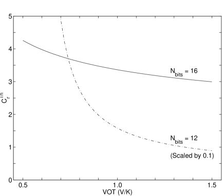
Figure 2: $C_{\mathrm{r}}^{\mathrm{Th}}$ as a function of ${\mathrm{VOT}}$ and $N_{\mathrm{bits}}$. It is assumed $\mbox{$V_{\mathrm{min}}$}=-10$ V, $\mbox{$V_{\mathrm{max}}$}=+10$ V and $\sigma_{l}=2\times 10^{-3}$ K. The curve for 12 bits is scaled by a factor 0.1 to allow a better comparison with the 16 bits curve.

From Eq. (9) it is possible to infer that the higher is the ${\mathrm{VOT}}$, (i.e. higher is the $\Delta T$ resolution) the worse is the compression rate, as already observed in Maris et al. (1998), Maris et al. (1999). The reason being the fact that as ${\mathrm{VOT}}$ is increased the number of quantization levels (i.e. of symbols) to be coded is increased and their distribution becomes more flat increasing $\overline{N_{\mathrm{bits}}^{\mathrm{out}}}$. Assuming that all the white noise is thermal in origin $\sigma_{l}\approx\sigma_{T}\approx 2\times 10^{-3}$ K. With the $\mathrm{adu}$ defined in equation (5) together with the typical values of $V_{\mathrm{min}}$ and $V_{\mathrm{max}}$ assumed therein and $\mbox{$N_{\mathrm{bits}}$}=16$ bits we have $\mbox{$C_{\mathrm{r}}^{\mathrm{Th}}$}\sim 11.09/(3.30+\ln\mbox{${\mathrm{VOT}}$})$. In conclusion, for $\mbox{${\mathrm{VOT}}$}=0.5$, $1.0$, $1.5$ V/K the $C_{\mathrm{r}}^{\mathrm{Th}}$ is respectively $4.26$, $3.36$, $3.00$. In addition figure 2 represents the effect of a reduction of $N_{\mathrm{bits}}$ on $C_{\mathrm{r}}^{\mathrm{Th}}$ compared to $C_{\mathrm{r}}^{\mathrm{Th}}$ for $\mbox{$N_{\mathrm{bits}}$}=16$.

5 Statistical Signal Analysis

A realistic estimation of the compression efficiency must be based on a quantitative analysis of the signal statistics, which includes: statistics of the binary representation (section 5.1), entropy section 5.2) and normality tests (section 5.3).

5.1 Binary Statistics

Most of the off-the-shelf compressors considered here do not handle 16 bits words, but 8 bits words. The 16 bits samples produced by the adc unit are splitted into two consecutive 8 bits (1 byte) words labeled: most significant bits (MSB) word and least significant bits (LSB) word. To properly understand the compression efficiency limits it is important to understand the statistical distribution of 8 bits words composing the quantized signal from LFI.

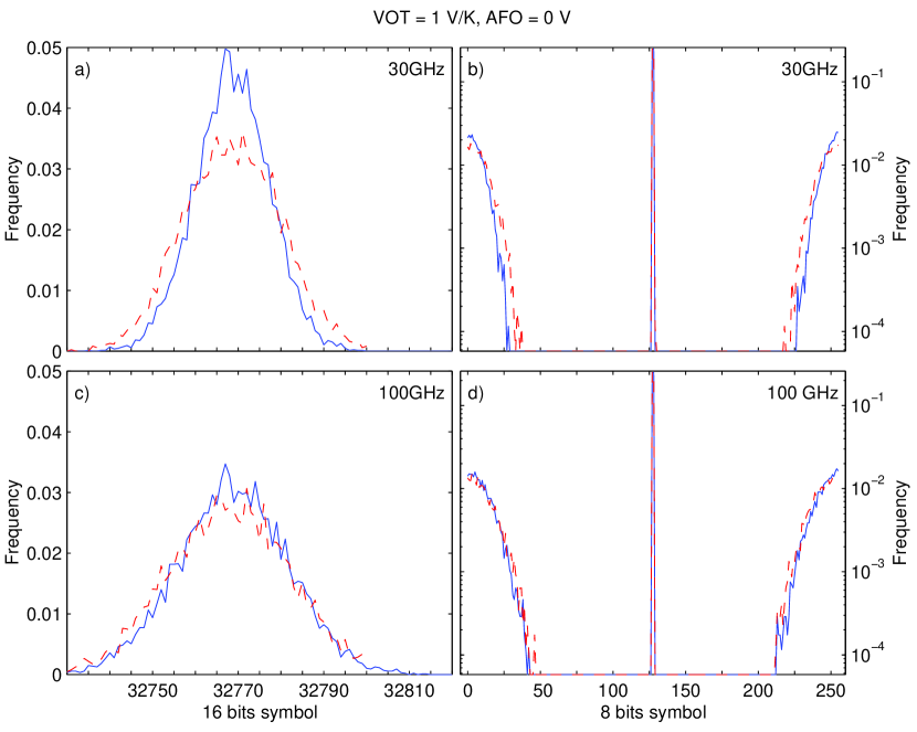
Figure 3: Statistical distribution of 8 and 16 bits words for LFI simulated signals. Upper row is for 30 GHz, lower row for 100 GHz. Left column are the distributions of 16 bits words from the quantized signals, right column is for 8 bits words from the quantized signal, full line is the distribution for pure white noise, dashed line is the distribution for the full signal.

Figure 3 represents the frequency distribution of symbols when the full data stream of 60 scan circles is divided into 8 bits words. Since for most of the samples the range spans over $\approx 64$ levels (5 bits) only the bytes corresponding to the MSB words assume a limited range of values producing the narrow spike in the figure. The belt shaped distribution at the edges is due to the set of LSB words. The distributions are quite sensitive to the quantization step, but do not change too much with the signal composition, the largest differences coming from the cosmological dipole contribution.

From the distribution in figure 3 one may wonder if it would not be possible to obtain a more effective compression splitting the data stream into two substreams: the MSB substream (with compression efficiency $C_{\mathrm{r}}^{\mathrm{MSB}}$) and the LSB substream (with compression efficiency $C_{\mathrm{r}}^{\mathrm{LSB}}$). Since the two components are so different in their statistics, with the MSB substream having an higher level of redundancy than the original data stream, it would be reasonable to expect that the final compression rate $2/(1/\mbox{$C_{\mathrm{r}}^{\mathrm{MSB}}$}+1/\mbox{$C_{\mathrm{r}}^{\mathrm{LSB}}$})$ be greater than the compression rate obtained compressing directly the original data stream. We tested this procedure taking some of the compressors considered for the final test. From these tests It is clear that $\mbox{$C_{\mathrm{r}}^{\mathrm{MSB}}$}>>\mbox{$C_{\mathrm{r}}$}$ but since most of the redundancy of the original data stream is contained in the MSB substream the LSB substream can not be compressed in an effective way, as a result $\mbox{$C_{\mathrm{r}}^{\mathrm{LSB}}$}<\mbox{$C_{\mathrm{r}}$}$ and $2/(1/\mbox{$C_{\mathrm{r}}^{\mathrm{MSB}}$}+1/\mbox{$C_{\mathrm{r}}^{\mathrm{LSB}}$})\mbox{$\stackrel{{{}_{<}}}{{{}_{\sim}}}$}\mbox{$C_{\mathrm{r}}$}$. So the best way to perform an efficient compression is to apply the compressor to the full stream without performing the MSB / LSB separation. Apart from these theoretical considerations, we performed some tests with our simulated data stream confirming these result.

5.2 Entropy Analysis

Equation (9) is valid in the limit of a continuous distribution of quantization levels. Since in our case the quantization step is about one tenth of the signal rms this is no longer true. To properly estimate the maximum compression rate attainable from these data we evaluate the entropy of the discretized signal using different values of the ${\mathrm{VOT}}$.

Our entropy evaluation code takes the input data stream and determines the frequency $f_{s}$ of each symbol $s$ in the quantized data stream and computing the entropy as: $-\sum_{s}f_{s}\log_{2}f_{s}$ where $s$ is the symbol index. In our simulation we take both 8 and 16 bits symbols ($s$ spanning over $0$, $\dots$, $255$ and $0$, $\dots$, $65535$). Since in our scheme the ADC output is 16 bits, we considered 8 bits symbols entropy both for the LSB and MSB 8 bits word and 8 bits entropy after merging the LSB and MSB significant bits set.

As expected, since $\mathrm{AFO}$ merely shifts the quantized signal distribution, entropy does not depend on $\mathrm{AFO}$. For this reason we take $\mbox{$\mathrm{AFO}$}=0$ V, i.e., no shift.

Table 2 reports the 16 bits entropy as a function of ${\mathrm{VOT}}$, composition and frequency. As obvious entropy, i.e. information content, increases increasing ${\mathrm{VOT}}$ i.e. quantization resolution. The entropy $H$ distribution allows to evaluate the $C_{\mathrm{r}}$ r.m.s. espected from different data streams realizations:

$$\mathrm{RMS}(\mbox{$C_{\mathrm{r}}$})\approx\mbox{$C_{\mathrm{r}}$}\frac{\mathrm{RMS}(H)}{H}.$$ (10)

Since data will be packed in chuncks of finite length it is important not only to study the entropy distribution for the entire data-stream, which will give an indication of the overall compressibility of the data stream as a wall, but also the entropy distribution for short packets of fixed length. So each data stream was splitted into an integer number of chunks of fixed length $l_{\mathrm{chunck}}$. For each chunck the entropy was measured, and the corresponding distribution of entropies for the given $L_{\mathrm{chunck}}$ as its mean and rms was obtained. We take $l_{\mathrm{chunk}}=16$, $32$, $64$, $135$, $8640$, $17280$ 16-bits samples, so each simulated $8640\times 60$ data stream will be splitted into 32400, 16200, 8100, 3840, 60, 30 chuncks. Small chunck sizes are introduced to study the entropy distribution as seen by most of the true compressors which do not compress one circle (8640 samples) at a time. Long chuncks distributions are usefull to understand the entropy distribution for the overall data-stream.

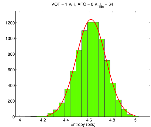
Figure 4: The entropy distribution per bunch for $l_{\mathrm{chunk}}=64$ samples, for the full signal at 30 GHz.

The entropy distribution per chunck is approximately described by a normal distribution (see figure 4), so the mean entropy and its r.m.s. are enough to characterize the results. Not however that the corresponding distribution of compression rates is not exactly normally distributed, however for the sake of this analysis we will assume that even the $C_{\mathrm{r}}$ distribution is normally distributed.

The mean entropy measured over one scan circle ($l_{\mathrm{chunk}}=8640$ samples) coincides with the entropy measured for the full set of 60 scan circles, the entropy r.m.s. being of the order of $10^{-2}$ bits. Consequently the expected r.m.s. for $C_{\mathrm{r}}$ compressing one or more circles at a time will be less than $1\%$.

The mean entropy and its rms are not independent quantities. Averaged entropy decreases as $L_{\mathrm{chunck}}$ decreases, but correspondingly the entropy r.m.s. increases. As a consequence the averaged $C_{\mathrm{r}}$ decreases decreasing $L_{\mathrm{chunck}}$, but the fraction of chunks in which the compressor performs significantly worst than in average increases. The overall compression rate, i.e. the $C_{\mathrm{r}}$ referred to the full mission, beeing affected by them.

5.3 Normality Tests

Since normal distribution of signals is assumed in 4 it would be interesting to fix how much the digitized signal distribution deviates from the normality. Also it would be important to characterize the influence of the 1/f noise and of the other signal components, especially the cosmic dipole, in the genesis of such deviations. To obtain an efficient compression it would be important that the samples are as more as possible statistically uncorrelated and normally distributed. In addition one should make sure that the detection chain does not cause any systematic effect which will introduce spurious non normal distributed components. This is relevant not only for the compression problem itself, which is among the data processing operations the least sensitive to small deviations from the normal distribution, but also in view of the future data reduction, calibration and analysis. For them the hypothesis of normality in the signal distribution is very important in order to allow a good separation of the foreground components. Last but not least, the hypothesis of conservation of normality along the detection chain, is important for the scientific interpretation of the results, since the accuracy expected from the Planck/LFI experiment should allow to verify if really the distribution of the CMB fluctuations at $l\mbox{$\stackrel{{{}_{>}}}{{{}_{\sim}}}$}14$ is normal, as predicted by the standard inflationary models, or as seems suggested by recent 4 years COBE/DMR results (Bromley & Tegmark (1999); Ferreira, Górsky, Magueijo (1999)).

For this reason a set of normality tests was applied to the different components of the simulated signal before and after digitization in order to characterize the signal statistics and its variation along the detection process. Of course this work may be regarded as a first step in this direction, a true calibration of the signal statistics will be possible only when the front end electronics simulator will be available. Those tests have furthermore the value of a preparation to the study of the true signal.

Normality tests were applied on the same data streams used for data compression. Given on board memory limits, it is unlikely that more than a few circles at a time can be stored before compression, so statistical tests where performed regarding each data stream for a given pointing, as a collection of 60 independent realizations of the same process. Of course this is only approximately true. The 1/f noise correlates subsequent scan circles, but since its r.m.s. amplitude per sample is typically about one-tenth of the white noise r.m.s. or less, these correlations can be neglected in this analysis.

Starting from the folded data streams a given normality test was applied to each set of 60 realizations for each one of the 8640 samples, transforming the stream of samples in a stream of test results for the given test. The cumulative distribution of frequency was then computed over the 8640 test results. Since 60 samples does not represent a large statistics, significant deviations from theorethically evaluated confidence levels are expected resulting in an excessive rejection or acceptation rates. For this reason each test was calibrated applying it to the undigitized white noise data stream. Moreover, in order to analyze how the normality evolves increasing the signal complexity, tests was repeated increasing the information content of the generated data stream.

To simplify the discussion we considered as a reference test the usual Kolmogorow - Smirnov D test from Press et al. (1986) and we fix a $95\%$ acceptance level. The test was “calibrated” using the MonteCarlo white noise generator of our mission simulator in order to fix the threshold level $D_{\mathrm{th}}$ as the $D$ value for which more than $95\%$ of our samples show $D\leq D_{\mathrm{th}}$. From Table 3 the quantization effect is evident, at twice the nominal quantization step ($\mbox{${\mathrm{VOT}}$}=2$ V/K) in $30\%$ of the samples (i.e. 2592 samples) the distribution of realizations deviates from a normal distribution ($D>D_{\mathrm{th}}$). Since the theoretical compression rate from eq. (9) is for a continuous distribution of levels ($\sigma\gg\Delta$) a smaller $C_{\mathrm{r}}$ should is expected. Since the deviation from the normal distribution is a systematic effect, for the sake of cosmological data analysis one may tune the D test to take account of the quantization. As an example, the third line in Tab. 3 reports the threshold for the quantized signal $D_{\mathrm{th}}^{\mathrm{Q}}$ for which $95\%$ of the quantized white noise samples are accepted as normal distributed. The line below represents the success rate for the full quantized signal. After the recalibration the test is able to recognize that in $95\%$ of the cases the signal is drawn from a normal distribution, but at the cost of a growth in the threshold $D$ which now is a function of the quantization step $\Delta$.

As for the entropy distribution and the binary statistics, even in this case most of the differences between the results obtained for a pure white noise signal and the full signals are explained by the presence of the cosmological dipole. However these simulations are not accurate enough to draw any quantitative conclusions about the distortion in the sampling statistics induced by digitization, but they suggest that to approximate the instrumental signal as a quantized white noise plus a cosinusoidal term associated to the cosmic dipole is more than adequate in order to understand the optimal loss-less compression rate achievable in the case of the Planck/LFI mission.

6 Quantization and Quantization Error

A possible solution to solve the bandwidth problem is to reduce the amount of information of the sampled signal i.e. its entropy. Independently from the way in which this is performed, the final compression strategy will be lossy, and the final reconstructed (uncompressed) signal will be corrupted with respect to the original one, degrading in some regard the experimental performances. In this regard, any sort of lossy compression may be seen as a kind of signal rebinning with a coarser resolution (quantization step) in $\Delta T/T$.

There are at least six aspects in Planck/LFI operations which may be affected by a coarser quantization:

1. $C_{l}$ and periodical signals reconstruction;

2. destriping;

3. foreground separation;

4. point like sources detection;

5. variable sources characterization;

6. tests for normality of CMB fluctuations.

Since the non linear nature of the quantization process, all of them are hard to be analytically evaluated and for this reason a specific simulation task is in progress for the Planck/LFI collaboration (White & Seiffert (1999), Maris et al. (2000)). However an heuristic evaluation for the point (1) by analytical means is feasible.

Quantization operates a convolution of the normal distribution of the input signal with the quantization operator $(x:\Delta)=$sign$(x)\Delta*floor(|x/\Delta|)$. If the quantization error: $(x-(x:\Delta))$ is uniformly distributed its expectation is $\Delta/2$ and its variance is $\Delta/\sqrt{12}$ (Kollár (1994)). Quantization over a large amount of samples may be regarded as an extra source of noise which will enhance the variance per sample. If the quantization error is statistically independent from the input quantized signal and if it may be added in quadrature to the white noise variance $\sigma_{WN}$, the total variance per sample will be $\approx\sigma_{WN}^{2}\left(1+\frac{\Delta^{2}/\sigma_{WN}^{2}}{12}\right)$. So for $\Delta\mbox{$\stackrel{{{}_{<}}}{{{}_{\sim}}}$}\sigma_{WN}$ the expected quantization r.m.s. is $\mbox{$\stackrel{{{}_{<}}}{{{}_{\sim}}}$}4\%$. From error propagation the relative error on the $C_{l}$ is (Maino (1999)):

$$\frac{\delta C_{l}}{C_{l}}=\sqrt{\frac{4\pi}{A}}\sqrt{\frac{2}{(2l+1)f_{sky}}}\left[1+\frac{\sigma^{2}\theta^{2}}{B_{l}^{2}C_{l}}\right]$$ (11)

so that the quantization contribution to the overall error will be small and dominated by the cosmic variance for a large set of $l$. However the application of such encouraging result must be considered carefully in a true experimental framework. Apart from the assumptions, it has to be demonstrated indeed that a large quantization error like this will not harm significantly the aforementioned aspects, moreover the impact of signal quantization will depend on how and in which point of the detection chain it will be performed.

7 Experimental Evaluation of Off-The-Shelf Compressors

This section describes the evaluation protocol and the experimental results of the compression of simulated data streams for Planck/LFI.

7.1 Evaluation Protocol

First tests were performed on a HP-UX workstation on four compressors (Maris et al. (1998)) but given the limited number of off-the-shelf compression codes for such platform, we migrated the compression pipeline on a Pentium III based Windows/NT workstation.

As described in section 2 the signal composition is defined by many components, both astrophysical and instrumental in origin. In particular, it is important to understand how each component or instrumental parameter, introducing deviations to the pure white noise statistics, affects the final compression rate.

To scan systematically all the relevant combinations of signal compositions and off-the-shelf compressors, a Compression Pipeline was created. The pipeline is based on five main components: the signal quantization pipeline, the signal database, the compression pipeline, the compression data base, the post-processing pipeline. The signal quantization pipeline performs the operations described in the upper part of figure 1. The simulated astrophysical signals are hold in a dedicated section of the signal archive, they are processed by the quantization pipeline and stored back in a reserved section of the signal archive. So quantized data streams are generated for each relevant combination of the quantization parameters, signal composition and sky pointing.

Each compressor is then applied by the compression pipeline to the full set of quantized signals in the signal archive. Results, in terms of compression efficiency as a function of quantization parameters are stored in the compression database. The statistical analysis of section 5 are performed with a similar pipeline.

Finally the post-processing pipeline scans the compression data base in order to produce plots, statistics, tables and synthetic fits. Its results are usually stored into one of the two databases.

The pipeline is managed by PERL 5.004 script files which drive FORTRAN, C, IDL programs or on-the-shelf utilities gluing and coordinating their activities. Up to $\approx 75\,000$ lines of repetitive code are required per simulation run. They are generated by a specifically designed Automated Program Generator (APG) written in IDL (Maris & Staniszkis (1998)). The APG takes as an input a table which specifies: the set of compressors to be tested, the set of quantization parameters to be used, the order in which to perform the scan of each parameter/compressor, the list of supporting programs to be used, other servicing parameters. The program linearizes the resulting parameter space and generates the PERL simulation code or, alternatively, performs other operations such as: to scan the results data base to produce statistics, plots, tables, and so on. The advantage of this method is that a large amount of repetitive code, may be quickly produced, maintained or replaced with a minor effort each time a new object (compressor, parameter or analysis method) is added to the system.

7.2 Experimental Results

Purpose of these compression tests is to give an upper limit to the lossless compression efficiency for LFI data and to look for an optimal compressor to be proposed to the LFI consortium.

A decision about the final compression scheme for Planck/LFI has not been taken yet and only future studies will be able to decide if the best performing one will be compatible with on-board operations (constrained by: packet independence and DPU capabilities) and will be accepted by the Planck/LFI collaboration.

For this reason up to now only off-the-shelf compressors and hardware where considered. To test any reasonable compression scheme a wide selection of lossless compression algorithms, covering all the known methods, was applied to our simulated data. Lacking a comprehensive criteria to fix a final compressor, as memory and CPU constrains, we report in a compact form the results related to all the tested compressors. We are confident that in the near future long duration flight balloon experiments as on-board electronics prototypes will provide us with a more solid base to test and improve the final compression algorithms looking at real data.

Tables 4, 5 list the selected compression programs. Since the behaviour (and efficiency) of each compressor is determined by a set of parameters one or more macro file operating a given combination of compressor code plus parameters is defined. It has to be noted that uses is a space qualified algorithm, based on Rice compression method, for which space qualified dedicated hardware already exists.

To evaluate the performances of each compressor, figures of merit are drawn like the one in figure 5 which shows the results for the best performing compressor: arith-n1. Looking at such figures it is possible to note as the compression efficiency does not depend much on the signal composition. This is true even when large, impulsive signals, as planets, affecting few samples over thousands are introduced. Again, this is a consequence of the fact that white noise dominates the signal, being the most important component to affect the compression efficiency. In this regard it has been speculated that the 1/f component should improve the correlation between neighborhood samples affecting the compression efficiency (Maris et al. (1998)) no relevant effect may be detected into our simulations. As an example from figure 5 for the 30 GHz signal the addition of the 1/f noise to the white noise data stream affects the final $C_{\mathrm{r}}$ for less than $0.5\%$.

The only noticeable (i.e. some $6\%$) effect due to an increase in the signal complexity, occurs when the cosmic dipole is added. In the present signal the dipole amplitude is comparable with the white noise amplitude ($\approx 3$ mK) so its effect is to distort the sample distribution, making it leptocurtic. As a consequence compressors, which usually work best for a normal distributed signal, becomes less effective. Since the dipole introduces correlations over one full scan circle, i.e. some $10^{3}$ samples, while compressors establish the proper coding table observing the data stream for a small set of consecutive samples (from some tens to some hundred samples), even a self adaptive compressor will likely loose the correlation introduced by the dipole. A proper solution to this problem is suggested in section 9. The other signal components do not introduce any noticeable systematic effect. The small differences shown by the figures of merit may be due to the compression variance and depend strongly on the compressor of choice. As an example a given compressor may be more effective to compress the simulated data stream with the full signal than the associated simpler data stream containing only white noise, 1/f noise, CMB and dipole. At the same time another compressor may show an opposite behaviour.

As shown by Figure 6, and as expected from eq. (9) increasing ${\mathrm{VOT}}$, i.e. increasing the quantization step, increases the compression rate. In addition $C_{\mathrm{r}}$ increases increasing $N_{\mathrm{c}}$ up to an $\approx 20\%$. The increase is noticeable for $\mbox{$N_{\mathrm{c}}$}<15$ and saturates after $\mbox{$N_{\mathrm{c}}$}=30$. On the contrary its dependence on the offset ($\mathrm{AFO}$) is negligible (less than $1\%$). For these reasons in the subsequent analysis the AFO dependency is neglected and the corresponding simulations are averaged.

7.3 Synthetical Description

The full data base of simulated compression results takes about 14 MBytes, for practical purposes it is possible to synthesize all this information using a phenomenological relation which connects $C_{\mathrm{r}}$ with $N_{\mathrm{c}}$ and ${\mathrm{VOT}}$ whose free parameters may be fitted using the data obtained from the simulations. In short:

$$\mbox{$C_{\mathrm{r}}^{\mathrm{Fit}}$}(\mbox{${\mathrm{VOT}}$},\mbox{$N_{\mathrm{c}}$})=\frac{\mbox{$C_{\mathrm{r},1}$}}{{\mathcal{I}}(\mbox{$N_{\mathrm{c}}$})+{\mathcal{S}}(\mbox{$N_{\mathrm{c}}$})\ln\left[\frac{\mathrm{VOT}}{1\;\mathrm{V/K}}\right]}$$ (12)

where $C_{\mathrm{r},1}$ is the $C_{\mathrm{r}}$ for $\mbox{$N_{\mathrm{c}}$}=1$, $\mbox{${\mathrm{VOT}}$}=1.0$ V/K, while ${\mathcal{I}(\mbox{$N_{\mathrm{c}}$})}$ and $\mathcal{S}(\mbox{$N_{\mathrm{c}}$})$ describe the $C_{\mathrm{r}}$ dependence on $N_{\mathrm{c}}$. In particular the relation is calibrated for any compressor imposing that $\mbox{$C_{\mathrm{r}}$}(\mbox{${\mathrm{VOT}}$}=1\;\mathrm{V/K},\mbox{$N_{\mathrm{c}}$}=1)=\mbox{$C_{\mathrm{r},1}$}$.

The linear dependency of $1/\mbox{$C_{\mathrm{r}}^{\mathrm{Fit}}$}$ over $\ln\mbox{${\mathrm{VOT}}$}$ is a direct consequence of equation (9), and is confirmed by a set of tests performed over the full set of our numerical results for the compression efficiency, the r.m.s. residual between the best fit (12) and simulated data being less than $1.5\%$, in almost the $92\%$ of the cases and less than $1\%$ in $72\%$ of the cases. The dependencies of its parameters $\mathcal{I}$ and $\mathrm{S}$ over $N_{\mathrm{c}}$ are obtained by a test-and-error method performed on our data set and we did not investigate further on their nature. For all practical purposes our analysis shows that these functions are well approximated by a series expansion:

$${\mathcal{I}}(\mbox{$N_{\mathrm{c}}$})\approx\exp\left(\sum_{k=1}^{2}A_{k}(\ln\mbox{$N_{\mathrm{c}}$})^{k}\right),$$ (13)

$${\mathcal{S}}(\mbox{$N_{\mathrm{c}}$})\approx\mbox{${\mathcal{S}}_{1}$}\exp\left(\sum_{k=1}^{5}B_{k}(\ln\mbox{$N_{\mathrm{c}}$})^{k}\right).$$ (14)

here ${\mathcal{S}}_{1}$, $A_{k}$ and $B_{k}$ are free parameters obtained by fitting the simulated data, in particular ${\mathcal{S}}_{1}$ is the slope for $\mbox{$N_{\mathrm{c}}$}=1$.

Since an accuracy of some percent in determining the free parameters of $\mbox{$C_{\mathrm{r}}^{\mathrm{Fit}}$}(\mbox{${\mathrm{VOT}}$},\mbox{$N_{\mathrm{c}}$})$ is enough, the fitting procedure was simplified as follow. For a given compressor, signal component, swap status, and $N_{\mathrm{c}}$ value $\mathcal{I}$ and $\mathcal{S}$ where determined by a $\chi^{2}$ fitting procedure. The list of $\mathcal{I}$ and $\mathcal{S}$ as a function of $N_{\mathrm{c}}$ have been fitted by using relations (13) and (14) respectively. The fitting algorithm tests different degrees of the polynomial in the aforementioned relations (up to 2 for $\mathcal{I}(\mbox{$N_{\mathrm{c}}$})$, up to 5 for $\mathcal{S}(\mbox{$N_{\mathrm{c}}$})$) stopping when the maximum deviation of the fitted relation respect to the data is smaller than $0.5\%$ for $\mathcal{I}$ or 0.0001 for $\mathcal{S}$, or when the maximum degree is reached.

Tables 6, 7, 8, 9 report the results of the compression exercise ordered for decreasing $C_{\mathrm{r},1}$. The first column is the name of compression macro (i.e. a given compression program with a defined selection of modificators and switches) as listed in tables: 4, 5. The third and fourth column are the fitted $C_{\mathrm{r},1}$and ${\mathcal{S}}_{1}$ as defined in: (12), (13), (14). From the $5^{\mathrm{th}}$ to the $7^{\mathrm{th}}$ columns and from the $8^{\mathrm{th}}$ to the $13^{\mathrm{th}}$ columns the polynomial degree and the expansion parameters for (13) and (14) are reported.

Many compressors are sensitive to the ordering of the Least and Most Significant Bytes of a 16 bits word in the computer memory and files. Two ordering conventions are assumed: UnSwapped i.e. Least Significant Byte is stored First or Swapped i.e. Most Significant Byte is stored First. As in Digital VAX/VMS Operating System, Microsoft Windows/NT operating system convention is Most Significant Byte first. For this reason each test was repeated twice, one time with the original data stream file with swapped bytes and the other after unswapping bytes. If the gain in $C_{\mathrm{r},1}$ after unswapping is bigger than some percent, unswapped compression is reported, otherwise the swapped one is reported. These two cases are distinct by the second column of tables 6, 7, 8, 9 which is marked with a y if unswapping is applied before compressing. It is interesting to note that not only 16 bits compressors, such as uses, are sensitive to swapping. Also many 8 bits compressors are sensitive to it, maybe that this is due to the fact that if the most probable 8 bits symbol is presented first at the compressor a slightly better balanced coding table is built.

It should be noted that the coefficients reported here are obtained compressing one or more full scan circles at a time, so their use to extrapolate $C_{\mathrm{r}}$ when each scan circle is divided in small chunks which are separately compressed has to be performed carefully, especially for $\mbox{${\mathrm{VOT}}$}\approx 0.5$ V/K where some extrapolated $C_{\mathrm{r}}$ grows instead of to decrease for a decreasing $N_{\mathrm{c}}$ as in most of the cases. However we did not investigate further the problem because the time required to perform all the tests over all the compressors increases decreasing $N_{\mathrm{c}}$, and because up to now a final decision about the packet length has not been made yet. Moreover, short data chunks introduce other constrains which are not accounted for by eq. (9) but which are discussed in section 8.

Apart from the choice of the best compressor, Tables 6, 7, 8, 9 allows interesting comparisons.

The performances of the arithmetic compression arith are very sensitive to changes in the coding order $n=0$, $\dots$, 7. The computational weight grows with $n$, while $C_{\mathrm{r}}$ is minimal at $n=0$, maximal for $n=1$ and decreases increasing $n$ further.

Both non-Adaptive Huffman (huff-c) and Adaptive Huffman (ahuff-c) are in the list of the worst compressors, considering both the pure white noise signal and the full signal.

We implemented the space-qualified uses compressor with a wide selection of combinations of its control parameters: the number of coding bits, the number of samples per block, the possibility to search for correlations between neighborhood samples. We report the tests for 16 bits coding only, changing the other parameters. Uses is very sensitive to byte unswapping, when not performed uses does not compress at all. On the other hand, opposite to arith the sensitivity of the final $C_{\mathrm{r}}$ to the various control parameters is small or negligible. In most cases $C_{\mathrm{r},1}$ differs of less than $0.01$ for changing the combination of control parameters, such changes are not displayed by the two digits approximation in the tables, but they are accounted for by the sorting procedure which fixes the table ordering. At 30 GHz most of the tested compressors cluster around $\mbox{$C_{\mathrm{r},1}$}=2.67$ and at this level arith-n3 is as good as uses. At 100 GHz the best uses macros clusters around $\mbox{$C_{\mathrm{r},1}$}=2.43$ - $2.44$, equivalent to arith-n2 performances. In our tests uses performs worst at 8 samples per block without correlation search, but apart from it, in our case the correlation search does not improve significantly the compression performances. Some commercial programs such as boa, bzip compress better than uses.

8 Further Constrains: Packet Independence and Packet Length

As an example of global constrains to the on-board compression we discuss the problems related to Packets Independence and Packets Length.

Data from the LFI must be packetized before being sent to Earth. Packets independence is considered to be a requirement, then each packet must be self-consistent, its loss or its erroneous transmission must not interfere with the data retrieval from subsequent packets. More over each packet must carry in “clear” format (i.e. uncompressed) all the information needed to decode its content. That is: each packet must contain its own decoding table or decoding information. A typical packet length is about some hundred of bytes, but smaller length may be planned if required; at the same time a typical decoding table holds something less than a hundred bytes leaving limited room for data.

In addition, for a fixed length $L_{\mathrm{u}}$ of a random input stream (expressed in bits) the output $L_{\mathrm{c}}$ will not be a constant but will change in time with respect to the averaged length $\mbox{$L_{\mathrm{u}}$}/\mbox{$C_{\mathrm{r}}$}$. Of course, it is not possible to predict in advance what will be the final length of a given bit stream. So either $L_{\mathrm{u}}$ is held fixed, loosing in compression efficiency, or $L_{\mathrm{u}}$ is adapted with some interactive method, maximizing the compression efficiency but at the cost of a significant slowing of the compression process.

In conclusion, the packets independence plus limited packet length prevents from sending the decoding table, leaving only two possibilities open: i) send the relevant bytes only (Maris (1999a)), ii) to use a predefined coding table (Maris (1999b)), both methods are described in the next section.

9 Proposed Coding and Compression Scheme

The basic principle of the first method named Least Significant Bits Packing (LSBP) is to send only those bits of the 16 bits output from the ADC which are affected by the signal and the noise. This is effective for the nominal mission since with the planned quantization step of 0.3 mK/adu, at one sigma the noise will fill about 21 levels, this will require at least 5 bits over 16 and it is reasonable to expect a final data flow equivalent to $\mbox{$C_{\mathrm{r},1}$}<3$. It is not possible to improve much the compression rate by compressing the resulting 5 bits data stream, since its entropy would be $H<5.4$ bits and $\mbox{$C_{\mathrm{r}}$}\mbox{$\stackrel{{{}_{<}}}{{{}_{\sim}}}$}1.08$.

In order to ensure the compression to be lossless all the samples exceeding the [$-\sigma$, $+\sigma$] (5 bits) range have to be sent separately coding at the same time: their position (address) in the stream vector and their value. So, for $\mbox{$N_{\mathrm{bits}}$}<16$ bits corresponding to a threshold $\mbox{$x_{\mathrm{th}}$}=2^{\mbox{$N_{\mathrm{bits}}$}}$, each group of samples stored into a packet is partitioned into two classes accordingly with their value $x$:

Regular Samples (RS)	$\langle$def$\rangle$	all those samples for which:	$|x|\leq\mbox{$x_{\mathrm{th}}$}$,
Spike Samples (SS)	$\langle$def$\rangle$	all those samples for which:	$|x|\geq\mbox{$x_{\mathrm{th}}$}.$

The coding process then consists of two main steps: i) to split the data stream in Regular and Spike Samples preserving the original ordering in the stream of Regular Samples, ii) to store (send) the first $N_{\mathrm{bits}}$ bits of the regular samples and, in a separated area, the 16 bits values and the location in the original data stream of each Spike Sample, i.e. Spike Samples will require more space to be stored than regular ones. The decoding process will be the reverse of this packing process.

In this scheme each packet will be divided into two main areas: the Regular Samples Area (RSA) which hold the stream of Regular Samples, the Spike Sample Area (SSA) which hold the stream of Spike Samples, plus a number of fields which will contain packing parameters such as: the number of samples, the number of regular samples, the offset, etc. Since the number of samples in each area will change randomly it will be not possible to completely fill a packet. The filling process will leave an empty area in the packet in average smaller than $N_{\mathrm{bits}}$.

In Maris (1999a) a first evaluation for the 30 GHz channel is given assuming that the signal is composed only of white noise plus the CMB dipole. As noticed in section 7.2 the cosmological dipole affects the compression efficiency reducing it of a small amount. To deal with it a possible solution would be to subdivide each data stream in packets, subtract to each measure of a given packet the integer average of samples (computed as a 16 bits integer number) and then compress the residuals. Each integer average will be sent to Earth together with the related packet where the operation will be reversed. Since all the numbers are coded as 16 bits integers all the operations are fully reversible and no round off error occurs. However it cannot be excluded that the computational cost of such operation will compensate the gain in $C_{\mathrm{r}}$.

Two schemes are proposed to perform the cosmological dipole self-adaptement. In Scheme A the average of samples in the packet are subtracted before coding and then sent separately. In Scheme B $x_{\mathrm{th}}$ is varied proportionally to the dipole contribution. Both of them assumes that the dipole contribution is about a constant over a packet length. From this assumption: $L_{p}\mbox{$\stackrel{{{}_{<}}}{{{}_{\sim}}}$}200$ samples i.e. $L_{p}<512$ bytes, since for $L_{p}>512$ bytes the cosmic dipole contribution can not be considered as a time constant. For larger packets a better modeling (i.e. more parameters) will be required in order not to degrade the compression efficiency.

A critical point is to fix the best $x_{\mathrm{th}}$, i.e. $N_{\mathrm{bits}}$, for a given signal statistics, coding scheme and packet length $L_{p}$. Even here $C_{\mathrm{r}}$ grows with the packet length but it does not change monotously with $x_{\mathrm{th}}$. An increase in $x_{\mathrm{th}}$ ($N_{\mathrm{bits}}$) decreases the number of spike samples, but increases the size of each regular sample. While the opposite occurs when $x_{\mathrm{th}}$ is decreased, and when $\mbox{$N_{\mathrm{bits}}$}<4$ bits $\mbox{$C_{\mathrm{r}}$}<1$. For both the schemes the optimality is reached for $\mbox{$N_{\mathrm{bits}}$}=6$ bits, but Scheme A is better than B, with: $\mbox{$C_{\mathrm{r}}$}(\mbox{{\em Scheme A}}$, $L_{p}=512\mbox{ bytes})=2.61$, $\mbox{$C_{\mathrm{r}}$}(\mbox{{\em Scheme B}}$, $L_{p}=512\mbox{ bytes})=2.29$.

Compared with arith-n1, this compression rate is smaller of about a 14 - 30%. This is due to two reasons: i) coding by a threshold cut is less effective than to apply an optimized compressor; ii) the results reported in tables 6, 7, 8, 9 refer to the compression of a full circle of data instead of a small packet, resulting in a higher efficiency. However, the efficiency of this coding method is similar to the efficiency of the bulk of the other true loss-less compressors tested up to now, and when the need to send a decoding table is considered, is even higher.

The second possible solution to the packeting problem is to use one or more standardized coding tables for the compression scheme of choice (Maris (1999b)). In this case the coding table would be loaded into the on-board computer before launch or time by time in flight and the table should be known in advance at Earth. Major advantages would be: 1. the coding table has not to be sent to Earth; 2. the compression operator will be reduced to a mapping operator which may be implement as a tabular search, driven by the input 8 or 16 bits word to be compressed; 3. any compression scheme (Huffman, arithmetic, etc.) may be implemented replacing the coding table without changes to the compression program; 4. the compression procedure may be easily written in C or the native assembler language for the on-board computer or, alternatively, a simple, dedicated hardware may be implemented and interfaced to the on-board computer. The disadvantages of this scheme are: 1. each table must reside permanently in the central computer memory unless a dedicated hardware is interfaced to it; 2. it is difficult to use adaptive schemes in order to tune the compressor to the input signal, as a consequence the $C_{\mathrm{r}}$ may be somewhat smaller than in the case of a true self-adapting compressor code.

The first problem may be circumvented limiting the length of the words to be compressed. In our case the data streams may be divided in chunks of 8 bits and the typical table size would be $\mbox{$\stackrel{{{}_{<}}}{{{}_{\sim}}}$}1$ Kbyte. Precomputed coding tables may be accurately optimized by Monte-Carlo simulations on ground or using signals from ground tests of true hardware.

The second problem may be overcome by using a preconditioning stage, reducing the statistics of the input signal to the statistics for which the pre-calculated table is optimized. In addition more tables may reside in the computer memory and selected looking to the signal statistics. With a simple reversible statistical preconditioner, about ten tables per frequency channel would be stored in the computer memory, so that the total memory occupation would be less than about 40 Kbytes. It cannot be excluded that the two methods just outlined cannot be merged.

10 Estimation of the Overall Compression Rate

The overall compression rate (efficiency) is the average of $C_{\mathrm{r}}$ ($\eta_{\mathrm{c}}$) over the full set of detectors. Appendix A illustrates the mathematical aspects of such average. From (A4):

$$\overline{\mbox{$C_{\mathrm{r}}$}}(\mbox{$N_{\mathrm{c}}$})=\left[\sum_{\nu}\frac{f_{\nu}}{\mbox{$C_{\mathrm{r}}$}_{,\nu}(\mbox{$N_{\mathrm{c}}$})}\right]^{-1}.$$ (15)

We will limit ourselves to the most probable case $\mbox{$N_{\mathrm{c}}$}=1$ and to the most effective compressor arith-n1. The compression parameters $C_{\mathrm{r},1}$ and ${\mathcal{S}}_{1}$ at 30 GHz and 100 GHz are derived from our simulations, while $C_{\mathrm{r},1}$ and ${\mathcal{S}}_{1}$ at 44 GHz and 70 GHz are obtained by linear interpolation of the simulated values as a function of $\ln\sigma_{\nu}$. After that we obtain:

$$\overline{\mbox{$C_{\mathrm{r}}$}}\approx\frac{2.66}{1+0.271\times\ln\mbox{${\mathrm{VOT}}$}}.$$ (16)

As expected the overall compression rate is dominated by the 100 GHz channel. Taking in account the conservative ${\mathrm{VOT}}$ distribution considered in equation (A8) the overall compression rate becomes: $\overline{\mbox{$C_{\mathrm{r}}$}}\approx 2.63$ which represents a $\approx 2\%$ correction only. It is likely that this correction will be even smaller, since the amplifiers gain will be adjusted in order to cover a smaller ${\mathrm{VOT}}$ interval. So this $2\%$ correction represents our greatest uncertainty in our estimation of the expected compression rate, and we may conservatively conclude that:

$$\overline{\mbox{$C_{\mathrm{r}}$}}_{,\mathrm{arith-n1}}\approx 2.65\pm 0.02$$ (17)

Recently a new evaluation of the expected instrumental sensitivity leads to some change in the expected white noise r.m.s.. These changes affect in particular the 30 GHz channel, but does not change significantly the 100 GHz channel so that the overall compression rate will be practically unaffected.

11 Conclusions

The expected data rate from the Planck Low Frequency Instrument is $\approx 260$ kbits/sec. The bandwidth for the scientific data download currently allocated is just $\approx 60$ kbit/sec. Assuming an equal subdivision of the bandwidth between the two instruments on-board Planck, an overall compression rate of a factor 8.7 is required to download all the data.

In this work we perform a full analysis on realistically simulated data streams for the 30 GHz and 100 GHz channels in order to fix the maximum compression rate achievable by loss-less compression methods, without considering explicitly other constrains such as: the power of the on-board Data Processing Unit, or the requirements about packet length limits and independence, but taking in account all the instrumental features relevant to data acquisition, i.e.: the quantization process, the temperature / voltage conversion, number of quantization bits and signal composition.

As a complement to the experimental analysis we perform in parallel a theoretical analysis of the maximum compression rate. Such analysis is based on the statistical properties of the simulated signal and is able to explain quantitatively most of the experimental results.

Our conclusions about the statistical analysis of the quantized signal are: I) the nominally quantized signal has an entropy $h\approx 5.5$ bits at 30GHz and $h\approx 5.9$ bits at 100GHz, which allows a theoretical upper limit for the compression rate $\approx 2.9$ at 30 Ghz and $\approx 2.7$ at 100 GHz. II) Quantization may introduce some distortion in the signal statistics but the subject requires a deepest analysis.

Our conclusions about the compression rate are summarized as follows: I) the compression rate $C_{\mathrm{r}}$ is affected by the quantization step, since greater is the quantization step higher is $C_{\mathrm{r}}$ (but worse is the measure accuracy). II) $C_{\mathrm{r}}$ is affected also by the stream length $L_{u}$, i.e. more circles are compressed better then few circles. III) the dependencies on the quantization step and $L_{u}$ for each compressor may be summarized by the empirical formula (12). A reduced compression rate $C_{\mathrm{r},1}$ is correspondingly defined. IV) the $C_{\mathrm{r}}$ is affected by the signal composition, in particular, by the white noise r.m.s. and by the dipole contribution, the former being the dominant parameter and the latter influencing $C_{\mathrm{r}}$ for less than $\approx 6\%$. The inclusion of the dipole contribution reduces the overall compression rate. The other components (1/f noise, CMB fluctuations, the galaxy, extragalactic sources) have little or no effect on $C_{\mathrm{r}}$. In conclusion, for the sake of compression rate estimation, the signal may be safely represented by a sinusoidal signal plus white noise. V) since the noise r.m.s. increases with the frequency, the compression rate $C_{\mathrm{r}}$ decreases with the frequency, for the LFI $\Delta\mbox{$C_{\mathrm{r}}$}/\mbox{$C_{\mathrm{r}}$}\mbox{$\stackrel{{{}_{<}}}{{{}_{\sim}}}$}10\%$. VI) the expected random r.m.s. in the overall compression rate is less than $1\%$. VII) we tested a large number of off-the-shelf compressors, with many combinations of control parameters so to cover every conceivable compression method. The best performing compressor is the arithmetic compression scheme of order 1: arith-n1, the final $C_{\mathrm{r},1}$ being 2.83 at 30 GHz and 2.61 at 100 GHz. This is significantly less than the bare theoretical compression rate (9) but when the quantization process is taken properly into account in the theoretical analysis, this discrepancy is largely reduced. VIII) taking into account the data flow distribution among different compressors the overall compression rate for arith-n1 is:

$$\overline{\mbox{$C_{\mathrm{r}}$}}_{,\mathrm{arith-n1}}\approx 2.65\pm 0.02$$

This result is due to the nature of the signal which is noise dominated and clearly excludes the possibility to reach the required data flow reduction through loss-less compression only.

Possible solutions deal with the application of lossy compression methods such as: on-board averaging, data rebinning, or averaging of signals from duplicated detectors, in order to reach an overall lossy compression of about a factor 3.4, which coupled with the overall loss-less compression rate of about 2.65 should allow to reach the required final compression rate $\approx 8.7$. However each of these solutions will introduce heavy constraints and important reduction of performances in the final mission design, so that careful and deep studies will be required in order to choose the best one.

Another solution to the bandwidth problem would be to apply a coarser quantization step. This has however the drawback of reducing the signal resolution in terms of $\Delta T/T$.

Lastly the choice of a given compressor cannot be based only on its efficiency obtained from simulated data, but also on the on-board available CPU and on the official ESA space qualification: tests with this hardware platform and other compressors will be made during the project development. Moreover, in the near future long duration flight balloon experiments and ground experiments (see Lasenby et al. (1998); De Bernardis & Masi (1998)) will provide a solid base to test and improve compression algorithms. In addition the final compression scheme will have to cope with requirements about packet length and packet independence. We discuss briefly this problems recalling two proposals (Maris (1999b), Maris (1999a)) which suggest solutions to cope with these constrains.

Appendix A Appendix: Formulation of the Final Data Flow

In this appendix we will discuss how to account for the distribution of the acquisition parameters between the different detectors in the computation of the overall compression rate. Since the formalism is simpler we will develop expressions for $\mbox{$\eta_{\mathrm{c}}$}=1/\mbox{$C_{\mathrm{r}}$}$ instead of $C_{\mathrm{r}}$.

We have pointed out in 5.2 that the compression efficiency is a random variable, whose distribution is a function of all those parameters which are relevant to fix the statistical distribution of the input signal. In our case: $\nu$, ${\mathrm{VOT}}$, $\mathrm{AFO}$, $N_{\mathrm{circ}}$ are the relevant parameters, so that the conditioned probability to have a compression efficiency in the range $\eta_{\mathrm{c}}$, $\mbox{$\eta_{\mathrm{c}}$}+d\mbox{$\eta_{\mathrm{c}}$}$ is:

$${\mathcal{P}}_{\nu,N_{\mathrm{Circ}}}\left(\mbox{$\eta_{\mathrm{c}}$}|\mbox{$\mathrm{AFO}$},\mbox{${\mathrm{VOT}}$}\right)d\mbox{$\eta_{\mathrm{c}}$}.$$ (A1)

This probability may be obtained by our MonteCarlo simulations for different combinations of $\mathrm{AFO}$, ${\mathrm{VOT}}$, $N_{\mathrm{circ}}$ and $\nu$. Then the averaged compression efficiency is:

$$\overline{\eta}_{\mathrm{{c}}\nu,N_{\mathrm{Circ}}}(\mbox{$\mathrm{AFO}$},\mbox{${\mathrm{VOT}}$})=\int_{0}^{+\infty}d\mbox{$\eta_{\mathrm{c}}$}\,\mbox{$\eta_{\mathrm{c}}$}\,{\mathcal{P}}_{\nu,N_{\mathrm{Circ}}}\left(\mbox{$\eta_{\mathrm{c}}$}|\mbox{$\mathrm{AFO}$},\mbox{${\mathrm{VOT}}$}\right).$$ (A2)

Of course we assumed that for any $\nu$, ${\mathrm{VOT}}$, $\mathrm{AFO}$, $N_{\mathrm{circ}}$ the probability distribution is integrable and normalized to 1, while the integration limits $0$, $+\infty$ are to be intended as formal. There are several detectors for any frequency channel, each one having its own $\mathrm{AFO}$ and ${\mathrm{VOT}}$, so distributions of $\mathrm{AFO}$ and ${\mathrm{VOT}}$ values may be guessed among the different detectors. Assuming they are integrable and normalized to 1 as well it is possible to compute the most probable $\mbox{$\overline{\eta}_{\mathrm{{c}}}$}_{\nu,N_{\mathrm{Circ}}}$ as ;

$$\mbox{$\overline{\eta}_{\mathrm{{c}}}$}_{\nu,N_{\mathrm{Circ}}}=\int_{\mathrm{AFO}_{\mathrm{min}}}^{\mathrm{AFO}_{\mathrm{max}}}d\mbox{$\mathrm{AFO}$}\,{\mathcal{P}}_{\nu}(\mbox{$\mathrm{AFO}$})\;\int_{\mathrm{VOT}_{\mathrm{min}}}^{\mathrm{VOT}_{\mathrm{max}}}d\mbox{${\mathrm{VOT}}$}\,{\mathcal{P}}_{\nu}(\mbox{${\mathrm{VOT}}$})\;\mbox{$\overline{\eta}_{\mathrm{{c}}}$}_{\nu,N_{\mathrm{Circ}}}(\mbox{$\mathrm{AFO}$},\mbox{${\mathrm{VOT}}$}).$$ (A3)

With this definition the final overall compression efficiency is:

$$\mbox{$\overline{\eta}_{\mathrm{{c}}}$}_{N_{\mathrm{Circ}}}=\sum_{\nu=30,44,70,100\mathrm{GHz}}f_{\nu}\mbox{$\overline{\eta}_{\mathrm{{c}}}$}_{\nu,N_{\mathrm{Circ}}}$$ (A4)

where $f_{\nu}$ is the partition function for the data flow through the different detectors, if $n_{\mathrm{dtc},\nu}$ is the number of detectors for the frequency channel $\nu$ (see Tab. I), $n_{\mathrm{dtc}}=\sum_{\nu=30,44,70,100\mathrm{GHz}}n_{\mathrm{dtc},\nu}=112$, is the total number of detectors and if the number of samples for frequency is a constant, then:

$$f_{\nu}=\frac{n_{\mathrm{dtc},\nu}}{112},$$ (A5)

so that for $\nu=30$, $44$, $70$ and 100 GHz respectively: $f_{\nu}=0.0714$, $0.1071$, $0.2143$ and $0.6071$, finally the expect data rate for each set of 60 circles is:

$$\overline{R}_{N_{\mathrm{Circ}}}=16\,\mathrm{bits}\;\times\;60\,\mathrm{circles}\;\times\;8640\,\mathrm{samples}\;\times\;112\,\mathrm{detectors}\;\times\;\mbox{$\overline{\eta}_{\mathrm{{c}}}$}^{N_{\mathrm{Circ}}}.$$ (A6)

Presently there are no data to know in advance the distribution of ${\mathrm{VOT}}$ and $\mathrm{AFO}$ values between the different detectors. For this reason in this work we assumed simply flat distributions, identical for each frequency for such parameters. More over, the $\mathrm{AFO}$ contribution is negligible, so that the variance introduced by this parameter is neglected. From (9) we assumed that the compression efficiency is approximately a linear function of $\ln\mbox{${\mathrm{VOT}}$}$ or:

$$\mbox{$\overline{\eta}_{\mathrm{{c}}}$}_{\nu,N_{\mathrm{Circ}}}(\mbox{${\mathrm{VOT}}$})\approx\mbox{$\overline{\eta}_{\mathrm{{c}}}$}_{\nu,N_{\mathrm{Circ}},1}+\mbox{$\dot{\overline{\eta}}_{\mathrm{{c}}}$}_{\nu,N_{\mathrm{Circ}}}\ln\mbox{${\mathrm{VOT}}$}$$ (A7)

where $\mbox{$\dot{\overline{\eta}}_{\mathrm{{c}}}$}_{\nu,N_{\mathrm{Circ}}}$ is the first derivative of $\mbox{$\overline{\eta}_{\mathrm{{c}}}$}_{\nu,N_{\mathrm{Circ}}}(\mbox{${\mathrm{VOT}}$})$ with respect to $\ln\mbox{${\mathrm{VOT}}$}$ computed for $\mbox{${\mathrm{VOT}}$}=1$ V/K, $\mbox{$\overline{\eta}_{\mathrm{{c}}}$}_{\nu,N_{\mathrm{Circ}},1}\equiv\mbox{$\overline{\eta}_{\mathrm{{c}}}$}_{\nu,N_{\mathrm{Circ}}}(\mbox{${\mathrm{VOT}}$}=1\;\mathrm{V/K})$. As an example, at 30 GHz for arith-n1 the full signal compression rate is $\mbox{$\overline{\eta}_{\mathrm{{c}}}$}_{\nu,N_{\mathrm{Circ}}}(\mbox{${\mathrm{VOT}}$})\approx 0.3534+0.287\times\ln\mbox{${\mathrm{VOT}}$}(\mathrm{K/V})$ with one interpolation error less than $0.2\%$. With these approximations eq. (A3) becomes

$$\mbox{$\overline{\eta}_{\mathrm{{c}}}$}_{\nu,N_{\mathrm{Circ}}}\approx\mbox{$\overline{\eta}_{\mathrm{{c}}}$}_{\nu,N_{\mathrm{Circ}},1}+\mbox{$\dot{\overline{\eta}}_{\mathrm{{c}}}$}_{\nu,N_{\mathrm{Circ}}}\int_{0.5\;\mathrm{V/K}}^{1.5\;\mathrm{V/K}}d\mbox{${\mathrm{VOT}}$}\,\frac{\ln\mbox{${\mathrm{VOT}}$}}{1.0\;\mathrm{V/K}}$$ (A8)

and after integration we obtain the final formula

$$\mbox{$\overline{\eta}_{\mathrm{{c}}}$}_{\nu,N_{\mathrm{Circ}}}\approx\mbox{$\overline{\eta}_{\mathrm{{c}}}$}_{\nu,N_{\mathrm{Circ}},1}-0.045229\cdot\mbox{$\dot{\overline{\eta}}_{\mathrm{{c}}}$}_{\nu,N_{\mathrm{Circ}}}$$ (A9)

for the case in the previous example: $\mbox{$\overline{\eta}_{\mathrm{{c}}}$}_{\nu,N_{\mathrm{Circ}}=2}\approx 0.3404$ which is equivalent to a compression efficiency $\approx 2.94$.

To understand the influence of the error in the ${\mathrm{VOT}}$ determination over the distribution on the final predictions the computation is made for a truncated (i.e. zero outside the ${\mathrm{VOT}}$ range of interest) normal distribution of ${\mathrm{VOT}}$. The r.m.s. for the ${\mathrm{VOT}}$ distribution is chosen in the ${\mathrm{VOT}}$ range [0.5, 1.5] V/K we obtain respectively $\mbox{$\overline{\eta}_{\mathrm{{c}}}$}_{\nu,N_{\mathrm{Circ}}}\approx 0.3494$, $0.3439$, $0.3420$; which corresponds to compression efficiencies: 2.86, 2.91, 2.92 respectively. Similar results are obtained with a quadratic ${\mathrm{VOT}}$ distribution. In conclusion these predictions are robust against the shape of the ${\mathrm{VOT}}$ distribution, at least for distributions which are symmetric around the nominal $\mbox{${\mathrm{VOT}}$}=1$ V/K value.

Table 1: Summary of LFI characteristics as recently revised by the LFI Consortium (Mandolesi et al. (1999)). Data rates are tabulated for the case of a sampling rate equal to 8640 samples per circle and constant time and frequency.

Center frequency $\nu$ [GHz]	30	44	70	100
Number of detectors $n_{\mathrm{dtc},\nu}$	8	12	24	68
Angular resolutions, FWHM [′]	33.6	22.9	14.4	10.0
Bandwidth [$\Delta\nu/\nu$]	0.2	0.2	0.2	0.2
$10^{6}\Delta T/T$	1.6	2.4	3.6	4.3
$\Delta T_{ant}$ [$\mu$K]	5.1	7.8	10.6	12.4
$\Delta T_{ant}$ [mK] per sampling and receiver	2.06	2.61	3.16	4.36
Number of samples for beam	13.4	9.2	5.8	4.0
Data rate for detector [Kb/sec]	2.3	2.3	2.3	2.3
Data rate for frequency [Kb/sec]	18.4	27.6	55.3	156.7
Uncompressed data rate partition function $f_{\nu}$ [$\%$]	7.14	10.71	21.43	60.71

Table 2: Entropy for 16 bits samples at 30 and 100 GHz, for only White Noise and Full Signal as a function of $L_{\mathrm{chunck}}$. Total Entropy refers to the entropy computed over the full set of samples ($8640\times 60$), Mean and RMS Entropy are the mean and RMS of different realizations of chunks of samples of length $L_{\mathrm{chunck}}$. The same for $C_{\mathrm{r}}$ columns. Here $C_{\mathrm{r}}$ are derived from the corresponding values of the entropy. The quantization step is $\Delta=0.305$ mK/adu.

30 GHz, White Noise
	Entropy (bits)			$C_{\mathrm{r}}$
$L_{\mathrm{chunck}}$	Total	Mean	RMS	Total	Mean	RMS
16	5.1618	3.5596	0.1989	3.10	4.49	0.251
32	5.1618	4.1815	0.1658	3.10	3.83	0.152
64	5.1618	4.6108	0.1262	3.10	3.47	0.095
135	5.1618	4.8791	0.0890	3.10	3.28	0.060
8640	5.1618	5.1561	0.0114	3.10	3.10	0.007
17280	5.1618	5.1589	0.0061	3.10	3.10	0.004
30 GHz, Full Signal
	Entropy (bits)			$C_{\mathrm{r}}$
$L_{\mathrm{chunck}}$	Total	Mean	RMS	Total	Mean	RMS
16	5.5213	3.5602	0.1982	2.90	4.49	0.250
32	5.5213	4.1849	0.1664	2.90	3.82	0.152
64	5.5213	4.6162	0.1278	2.90	3.47	0.096
135	5.5213	4.8885	0.0893	2.90	3.27	0.060
8640	5.5213	5.5119	0.0176	2.90	2.90	0.009
17280	5.5213	5.5157	0.0118	2.90	2.90	0.006
100 GHz, White Noise
	Entropy (bits)			$C_{\mathrm{r}}$
$L_{\mathrm{chunck}}$	Total	Mean	RMS	Total	Mean	RMS
16	5.7436	3.6962	0.1740	2.79	4.33	0.204
32	5.7436	4.4174	0.1521	2.79	3.62	0.125
64	5.7436	4.9627	0.1230	2.79	3.22	0.080
135	5.7436	5.3354	0.0875	2.79	3.00	0.049
8640	5.7436	5.7352	0.0115	2.79	2.79	0.006
17280	5.7436	5.7394	0.0063	2.79	2.79	0.003
100 GHz, Full Signal
	Entropy (bits)			$C_{\mathrm{r}}$
$L_{\mathrm{chunck}}$	Total	Mean	RMS	Total	Mean	RMS
16	5.8737	3.6970	0.1734	2.72	4.33	0.203
32	5.8737	4.4186	0.1526	2.72	3.62	0.125
64	5.8737	4.9655	0.1224	2.72	3.22	0.079
135	5.8737	5.3419	0.0887	2.72	3.00	0.050
8640	5.8737	5.8604	0.0180	2.72	2.73	0.008
17280	5.8737	5.8655	0.0127	2.72	2.73	0.006

Table 3: Quantization Effect on the Kolmogorow - Smirnov D test applied to simulated data, $\Delta$ is the quantization step.

	$\Delta$ (mK/adu)
	1.220	0.610	0.406
${\mathcal{F}}(D<0.1475,\;\mathrm{White\;Noise})$	0.28	0.70	0.84
${\mathcal{F}}(D<0.1475,\;\mathrm{Signal})$	0.27	0.71	0.86
$D_{\mathrm{95}}^{\mathrm{Q}}$	0.2449	0.1851	0.1678
${\mathcal{F}}(D<D_{\mathrm{95}}^{\mathrm{Q}},\;\mathrm{Signal})$	0.95	0.95	0.95

Table 4: Tested compressors and related parameters. The Macro column contains the names of the macros running a given compression Code with a given combination of Parameters

Macro	Code	Parameters	Note
ahuff-c	ahuff-c		Adaptive Huffman Nelson & Gailly (1996)
AR	ar
arc	arc
arha	arhangel		http://www.geocities.com/SiliconValley/Lab/6606
arhaASC	”	-1	ASC method
arhaHSC	”	-2	HSC method
arith-c	arith-c		Arithmetic coding Nelson & Gailly (1996)
arith-n	arith-n		Adaptive Arithmetic Coding (AC) Nelson & Gailly (1996)
arith-n0	”	-o 0	Zeroth order Arithmetic coding
arith-n1	”	-o 1	First order AC
arith-n2	”	-o 2	Second order AC
arith-n3	”	-o 3	Third order AC
arith-n4	”	-o 4	Fourth order AC
arith-n5	”	-o 5	Fifth order AC
arith-n6	”	-o 6	Sixth order AC
arith-n7	”	-o 7	Seventh order AC
arj	arj
arj0	”	-m 0	method 0 (no compression)
arj1	”	-m 1	method 1
arj2	”	-m 2	method 2
arj3	”	-m 3	method 3
arj4	”	-m 4	method 4
boa	boa
bzip	bzip2090
bziprb	”	–repetitive-best	best compression of repetitive blocks
bziprf	”	–repetitive-fast	fast compression of repetitive blocks
gzip1	gzip	-1	fast compression
gzip9	”	-9	best compression
huff-c	huff-c		Hauffman Nelson & Gailly (1996)
jar	jar32
jar1	”	-m1	method 1
jar2	”	-m2	method 2
jar3	”	-m3	method 3
jar4	”	-m4	method 4
lha	lha
lzss	lzss
lzw12	lzw12
lzw15v	lzw15v

Table 5: See table 4.

Macro	Code	Parameters	Note
pkzip	pkzip		from PKWARE
pkzip-ef	”	-ef	fast compression
pkzip-en	”	-en	normal compression
pkzip-es	”	-es	super fast compression
pkzip-ex	”	-ex	extra compression
rar-m0	rar	-m0	level 0 compression
rar-m1	”	-m1	level 1 compression
rar-m2	”	-m2	level 2 compression
rar-m3	”	-m3	level 3 compression
rar-m4	”	-m4	level 4 compression
rar-m5	”	-m5	level 5 compression
splint	splint
SZIP00	szip		Rice Algorithm and Rice compression chip simulator
szip0ec	”	-ec	entropy coding compression mode
szip0nu	”	-nn	nearest neighbor compression mode
szipc0	”	-chip	compress exactly as chip
SZIPCEC	”	-chip -ec	as szip0ec + chip compression
SZIPCNU	”	-chip -nn	as szip0nu + chip compression
uses	uses	-n 16 -s 64 -rr	Universal Source Encoder for Space
			16 bits per sample,
			64 samples for scanline,
			correlates near samples (CNS)
uses008	”	-n 16 -s 8 -j 8	8 samples, 8 samples per block
uses008rr	”	-n 16 -s 8 -rr -j 8	as uses008 + CNS
uses016	”	-n 16 -s 16	16 samples per block
uses016rr	”	-n 16 -s 16 -rr	16 samples per block + CNS
uses032	”	-n 16 -s 32	32 samples per block
uses032rr	”	-n 16 -s 32 -rr	32 samples per block + CNS
uses064	”	-n 16 -s 64	64 samples per block
uses064rr	”	-n 16 -s 64 -rr	64 samples per block + CNS
uses320	”	-n 16 -s 320	320 samples per block
uses320rr	”	-n 16 -s 320 -rr	320 samples per block + CNS
uses960	”	-n 16 -s 960	960 samples per block
uses960rr	”	-n 16 -s 960 -rr	960 samples per block + CNS
zoo	zoo

Table 6: Compression Rates at 30 GHz, white noise only

Table 7: Compression Rates at 30 GHz, full signal

Table 8: Compression Rates at 100 GHz, white noise only

Table 9: Compression Rates at 100 GHz, full signal

Figure 5: Figures of merit for the arithmetic compression of order 1 (arith-n1) for 30 GHz and 100 GHz channels. Here $\mbox{$\mathrm{AFO}$}=0$ V, $\mbox{${\mathrm{VOT}}$}=1.0$ V/K, $\mbox{$N_{\mathrm{c}}$}=1$. The compression efficiency is plotted as a function of the incremental complexity of the signal composition: wn means white noise only, +1/f plus 1/f, +cmb plus CMB, +dipo plus dipole, +gal plus galaxy, +ex plus extragalactic sources.

Figure 6: Compression rates for arith-n1 as a function of the ${\mathrm{VOT}}$ and $N_{\mathrm{c}}$ for a full simulated signal (wn + 1/f + dp + cmb + dipo + gal + ex) (see also figure 5 for details). From top to bottom: Squares: $\mbox{${\mathrm{VOT}}$}=1.5$ V/K, Diamonds: $\mbox{${\mathrm{VOT}}$}=1.0$ V/K, Triangles: $\mbox{${\mathrm{VOT}}$}=0.5$ V/K.

References

- Bersanelli et al. (1996) Bersanelli, M., et al. 1996, COBRAS/SAMBA, Rep. Phase A Study, ESA D/SCI(96)3
- Bromley & Tegmark (1999) Bromley, B. C., Tegmark M., 1999, ApJsubmitted
- Burigana et al. (1997a) Burigana, C., et al. 1997a, MNRAS, 287, L17
- Burigana et al. (1997b) Burigana, C., et al. 1997b, Int. Rep. TeSRE/CNR 198/1997
- Burigana et al. (1998a) Burigana, C., et al. 1998a, A&AS, 130, 551
- Burigana et al. (1998b) Burigana, C., et al. 1998b, submitted to Ap. Lett. Comm.
- Danese et al. (1987) Danese, L., et al. 1987, ApJ, 318, L15
- De Bernardis & Masi (1998) De Bernardis, P., & Masi S., Proceedings of the XXXIIIrd Rescontres de Moriond, Les Arcs, France, January 17-24, 1998, p. 209
- De Zotti & Toffolatti (1998) De Zotti, G. & Toffolatti, L., 1998, Astrophys. Lett., in press
- Ferreira, Górsky, Magueijo (1999) Ferreira, P. G., Górski, K. M., Magueijo J., 1999, astro-ph/9904073
- Fixsen et al. (1996) Fixsen, D.J., et al. 1996, ApJ, 473, 576
- Franceschini et al. (1994) Franceschini, A., et al.1994, ApJ, 427, 140
- Gaztñaga et al. (1998) Gaztñaga, E., et al. 1998, Ap. Lett. Comm. in press (also LFI-IEEC-TN-002.0)
- Haslam et al. (1982) Haslam, G.T., et al. 1982, A&AS, 47, 1
- Impey & Neugebauer (1988) Impey, C.D. & Neugebauer,G. 1988, AJ, 95, 307
- Jonas et al. (1998) Jonas, J.L., et al. 1998, MNRAS, 297, 997
- Kollár (1994) Kollár, I., 1994, IEEE Trans. Intrum. and Measur., 43, 5, 733
- Lasenby et al. (1998) Lasenby, A., et al. (1998), Proceedings of the XXXIIIrd Rescontres de Moriond, Les Arcs, France, January 17-24, 1998, p. 221
- Maino (1999) Maino, D., Ph.D. Thesis, ISAS, October 1999
- Maino et al. (1999) Maino, D., et al. 1999, A&AS, 140, 383
- Mandolesi et al. (1998a) Mandolesi, N., et al. 1998a, Low Frequency Instrument for Planck, Proposal submitted to European Space Agency
- Mandolesi et al. (1998b) Mandolesi, N., et al. 1998b, submitted to Ap. Lett. Comm.
- Mandolesi et al. (1999) Mandolesi, N., et al. 1999, Planck Low Frequency Instrument, Instrument Science Verification Review, LFI Design Report, October 1999
- Maris & Staniszkis (1998) Maris, M. & Staniszkis, M., 1998, ADASS VIII, 470, Eds. D.M. Mehringer, R. Plante & D.A. Roberts
- Maris et al. (1998) Maris, M., et al. 1998, ADASS VIII, 145, Eds. D.M. Mehringer, R. Plante & D.A. Roberts
- Maris et al. (1999) Maris, M., et al. 1999, proceedings of the XLIII National Congress of the Italian Astronomical Society held in Naples, Italy from 4 to 8 May 1999, edt. R. Agatino, in press.
- Maris (1999a) Maris, M., 1999a, OAT-Tech. Rep., 55/99, PL-LFI-OAT-TN-005
- Maris (1999b) Maris, M., 1999b, OAT-Tech. Rep., 56/99, PL-LFI-OAT-TN-006
- Maris et al. (2000) Maris, M., et al. 2000, in progress
- Mather et al. (1999) Mather, J. C., et al. , 1999, ApJ, 512, 511
- Muciaccia et al. (1997) Muciaccia, P.F., Natoli, P. & Vittorio, N., 1997, ApJ, 488, L63
- Nelson & Gailly (1996) Nelson, M., Gailly, J.L., 1996, The Data Compression Book IInd edt., M & T Books, New York, USA
- Platania et al. (1998) Platania, P., et al. 1998, ApJ, 505, 473
- Press et al. (1986) Press, W. H., Flannery, B. P., Teukolsky S. A., Vetterling, W. T., Numerical Recipes Cambridge University Press, 1986, Cambridge USA
- Puget et al. (1996) Puget, J.-L., et al. 1996, A&A, 308, 5
- Puget et al. (1998) Puget, J.-L., et al. 1998, High Frequency Instrument for Planck, Proposal submitted to European Space Agency
- Reich & Reich (1986) Reich, P. & Reich, W., 1986, A&AS, 63, 205
- Schlegel et al. (1998) Schlegel D.J., et al. 1998, ApJ, 500, 525
- Seiffert et al. (1997) Seiffert, M., et al. 1997, sub. to The Rev. of Sci. Instr.
- Seiffert (1999) Seiffert, M., 1999, private communication
- Toffolatti et al. (1998) Toffolatti, L., et al. 1998, MNRAS, 297, 117
- Witebsky (1978) Witebsky, C., 1978, private communication
- White & Seiffert (1999) White, M., Seyfert, W., 1999, LFI internal report