COMPTON SCATTERING IN ULTRA-STRONG MAGNETIC FIELDS:
NUMERICAL AND ANALYTICAL BEHAVIOR
IN THE RELATIVISTIC REGIME

Abstract

This paper explores the effects of strong magnetic fields on the Compton scattering of relativistic electrons. Recent studies of upscattering and energy loss by relativistic electrons that have used the non-relativistic, magnetic Thomson cross section for resonant scattering or the Klein-Nishina cross section for non-resonant scattering do not account for the relativistic quantum effects of strong fields ($>4\times 10^{12}$ G). We have derived a simplified expression for the exact QED scattering cross section for the broadly-applicable case where relativistic electrons move along the magnetic field. To facilitate applications to astrophysical models, we have also developed compact approximate expressions for both the differential and total polarization-dependent cross sections, with the latter representing well the exact total QED cross section even at the high fields believed to be present in environments near the stellar surfaces of Soft Gamma-Ray Repeaters and Anomalous X-Ray Pulsars. We find that strong magnetic fields significantly lower the Compton scattering cross section below and at the resonance, when the incident photon energy exceeds $m_{e}c^{2}$ in the electron rest frame. The cross section is strongly dependent on the polarization of the final scattered photon. Below the cyclotron fundamental, mostly photons of perpendicular polarization are produced in scatterings, a situation that also arises above this resonance for sub-critical fields. However, an interesting discovery is that for super-critical fields, a preponderance of photons of parallel polarization results from scatterings above the cyclotron fundamental. This characteristic is both a relativistic and magnetic effect not present in the Thomson or Klein-Nishina limits.

p

                                                            Astrophysical Journal, in press,

                                                            Vol. 541, September 20, 2000

1 INTRODUCTION

Recent observations are providing evidence for the existence of isolated neutron stars having ultra-strong magnetic fields. Assuming that the spin-down of isolated neutron stars is a result of electromagnetic dipole radiation, the measured period and the period derivative give the strength of the surface magnetic field as $B_{o}=6.4\times 10^{19}(P\dot{P})^{1/2}$ (Shapiro & Teukolsky 1983 and Usov & Melrose 1995). Typical radio pulsars have period and period derivative distributions (from the Princeton Pulsar Catalogue: Taylor, Manchester, & Lyne 1993) suggesting magnetic field strengths between $10^{11}$ and $10^{13}G$, with about two dozen pulsars having spin-down fields greater than $10^{13}G$; the highest to date is $B_{o}=1.1\times 10^{14}G$, a product of the Parkes multi-beam survey (Camilo et al. 1999). Although there have not been any radio pulsars detected with a magnetic field much exceeding $B_{o}=10^{14}G$ (perhaps with the exception of the unconfirmed observation of SGR 1900+14; Shitov 1999; Shitov, Pugachev & Kutuzov 2000), growing evidence for a new class of isolated neutron stars with ultra-strong magnetic fields ($B_{o}>10^{14}G$) has come from the observations of Soft Gamma-Ray Repeaters (SGRs) and Anomalous X-ray pulsars (AXPs). The five known SGRs are transient sources that undergo repeated outbursts of gamma rays and all have been associated with young ($t<10^{5}yr.$) supernova remnants. Last year, Kouveliotou et al. (1998a) detected a 7.47 s period in quiescent emission of SGR1806-20 in the X-ray band. Recently, Hurley et al. (1999) detected a periodicity of 5.16 s for SGR1900+14 during a giant burst having an energy of $\sim 10^{45}erg$. Kouveliotou et al. (1999) also observed the same period in the quiescent X-ray emission. Assuming dipole radiation torques, the measured period derivatives imply surface magnetic fields between $10^{14}-10^{15}G$, well above the quantum critical field, $B_{\rm cr}=4.4\times 10^{13}G$.

Evidence for ultra-strong magnetic fields has also come from observations of AXPs, a group of six or seven X-ray pulsars with supersecond periods that exhibit anomalous characteristics in comparison to the properties of accreting X-ray pulsars. The lack of optical counterparts and orbital Doppler shifts (Steinle et al. 1987, Mereghetti et al. 1992 and Mereghetti & Stella 1995) suggest that these objects are isolated pulsars. Their more-or-less steady spin-down and young characteristic ages, $t<10^{5}yr.$ (Vasisht & Gotthelf 1997), support this assertion. Several AXPs have been associated with young supernova remnants, also suggesting neutron star origin. The AXPs are bright X-ray sources with luminosities, $L_{X}\sim 10^{35}erg/s$, far exceeding their spin-down luminosity. This energetics issue has motivated Thompson & Duncan (1996) and Kulkarni & Thompson (1998) to suggest that, unlike rotation-powered pulsars, the X-ray and particle emission in AXPs is powered by a decay of the magnetic field in the stellar interior.

Various studies indicate that inverse Compton scattering (ICS) plays a significant role in the magnetospheric physics of strongly magnetized neutron stars. Relativistic electrons accelerated above the polar cap can Compton scatter off thermal radiation from the neutron star surface, producing high energy gamma rays that can power pair cascades. Daugherty & Harding (1989) found that in the presence of a strong magnetic field, resonant scattering greatly increases electron energy losses over those of non-resonant scattering, making Compton scattering efficient even at lower temperatures. Recent studies have indicated the importance of resonant Compton scattering over curvature radiation in pulsar polar cap acceleration models. Luo (1996) and Zhang et al. (1997) observed that if the polar cap temperature and the magnetic field are sufficiently high, the thickness of the accelerating gap is limited more efficiently by pairs from Compton scattered photons than by pairs from curvature radiation photons. Harding & Muslimov (1998) considered ICS by the trapped, back flowing positrons and found that the pairs from the ICS photons may cause surface acceleration gaps to be unstable, forcing them to higher altitudes. These studies indicate the evolving, critical role of Compton scattering in polar cap models.

Compton scattering is also very important in SGR radiation models. The highly super-Eddington luminosities of the bursts ensures high densities of both photons and particles, so that scattering will be a critical factor. Paczynski (1992) proposed that the lower scattering cross section below the resonance in the strong magnetic field (for photons in the perpendicular polarization mode) could allow super-Eddington luminosities. However, Miller et al. (1995) argued that scattering into the parallel mode keeps the radiation pressure high, and thus the effective Eddington luminosity lower, in hydrostatic atmospheres. In Thompson & Duncan’s (1995) model for the radiation from SGR bursts, Compton scattering plays a critical role in establishing equilibrium between pairs and photons and in the spectral formation. Compton scattering may also be important in the photon splitting cascade model for SGR burst emission (Baring 1995, Harding, Baring & Gonthier 1996 and Harding, Baring & Gonthier 1997). The issues raised and discussed by these papers all depend critically on the polarization state and the angular distribution of the photons involved in a scattering event.

The full QED expressions for the relativistic, magnetic cross section of Compton scattering were derived separately by Daugherty and Harding (1986, hereafter DH86), and Bussard et al. (1986) and discussed by Meszaros (1992). Because of the complexity of the expressions, they have been applied to the study of relativistic Compton scattering in high magnetic fields only for the case of a one-dimensional, thermal electron distribution. These studies (Alexander & Meszaros 1989, 1991, Harding & Daugherty 1991, Araya & Harding 1996, 1999) focussed on models of cyclotron line formation in accreting neutron star atmospheres and gamma-ray bursts. The inverse Compton scattering models for pulsars and SGRs described in the preceeding paragraphs involve non-thermal, highly relativistic electrons. Such models have not to date incorporated the QED scattering cross sections, because the larger length scales require treatment of field inhomogeneity (unlike the cyclotron line scattering models which assume homogeneous fields). Consequently, these inverse Compton scattering studies have had to approximate the scattering rates by a combination of the Klein-Nishina cross section for non-resonant Compton scattering and the non-relativistic (Thomson) limit (Canuto, Lodenquai, & Ruderman 1971, Blandford & Scharlemann 1976 and Herold 1979) for resonant Compton scattering. As a result, they do not include the quantum relativistic effects of a strong magnetic field ($B>0.1$, where here and throughout the paper $B$ is given in units of the critical field, $B_{\rm cr}=m_{e}^{2}c^{3}/e\hbar=4.414\times 10^{13}$Gauss).

It is the purpose of this paper to explicitly present the major features of Compton scattering in strong sub-critical and super-critical magnetic fields, providing a development of simplified expressions for the magnetic scattering cross section, to facilitate applications to environments near the surfaces of pulsars, SGRs or AXPs. We extend the work of DH86 by obtaining expressions suitable for rapid computation of the polarized, differential and integrated cross sections, applicable to Compton scattering of highly relativistic electrons moving along the magnetic field. In this case, broadly applicable in astrophysical problems, photons propagate along the field in the electron rest frame. In this specialized axisymmetric case, there is a degeneracy between polarization transitions $\perp\rightarrow\parallel$ and $\parallel\rightarrow\parallel$, with a similar identity of cross sections for the modes $\perp\rightarrow\perp$ and $\parallel\rightarrow\perp$. Below the cyclotron fundamental, mostly $\perp$-photons are produced in scatterings, a situation that also pertains above this resonance for sub-critical fields. However, an interesting discovery of this paper is that for super-critical fields, the reverse situation arises above the cyclotron fundamental, and a preponderance of photons of parallel polarization results from scatterings. We derive an analytic approximation that describes well the integrated cross section for Compton scattering in both sub-critical and super-critical magnetic fields. The effects of the strong magnetic fields on the angle-integrated cross sections and angular distributions of scattered photons is also studied, noting in particular significant differences for large scattering angles between the high energy magnetic forms and the non-magnetic Klein-Nishina results. Finally, we discuss the impact of this field-dependent cross section on the simulation of acceleration and cascade processes in pulsars and SGR sources.

2 QED COMPTON SCATTERING CROSS SECTION

The present study follows the development of DH86, applying their work to a particular case for scattering of relativistic electrons. The expressions developed in this paper use the Johnson & Lippmann (1949) electron wavefunctions. Graziani (1993) and Graziani, Harding & Sina (1995) have indicated that the choice of these wavefunctions do not diagonalize the magnetic moment operator parallel to the external field resulting in some limitations and inaccuracies when spin-dependent cross sections are used. Therefore, in this work, we present results that are spin-averaged. We will further discuss this issue in section 4. The differential cross section in the rest frame of the electron is given in equation (11) of DH86, with the denominator term later corrected in Harding & Daugherty (1991), by the expression

$${{d\sigma}\over{d\Omega^{\prime}}}={{3\sigma_{\rm T}}\over{16\pi}}{{\omega^{\prime}\;e^{-(\omega^{\prime 2}\sin^{2}\theta^{\prime}+\omega^{2}\sin^{2}\theta)/2B}}\over{\omega\left({1+\omega-\omega^{\prime}-(\omega\cos\theta-\omega^{\prime}\cos\theta^{\prime})\cos\theta^{\prime}}\right)\left({2+\omega-\omega^{\prime}}\right)}}\left|{\sum\limits_{n=0}^{\infty}{\left[{F_{n}^{(1)}e^{i\Phi_{1}}+F_{n}^{(2)}e^{i\Phi_{2}}}\right]}}\right|^{2}.$$ (1)

While photon-electron interactions may excite electrons above the ground state in this case (to quantum numbers $\ell\geq 0$), the initial electron is assumed to be in its ground state with $m=0$ Landau state and its spin anti-parallel to the magnetic field. This assumption is valid as the synchro-cyclotron decay of excited states occurs during an extremely short time-scale. The incident and scattered photon energies denoted by, $\omega$ and $\omega^{\prime}$, respectively are in units of the electron rest mass energy, $m_{e}c^{2}$. The incident and scattered angles are denoted by $\theta$ and $\theta^{\prime}$, respectively, with respect to the z-axis determined by the direction of the magnetic field. The common phase factors are given by

$$\Phi_{1}=-\Phi_{2}={{\omega\omega^{\prime}\sin\theta\sin\theta^{\prime}}\over{2B}}\sin(\phi-\phi^{\prime}).$$ (2)

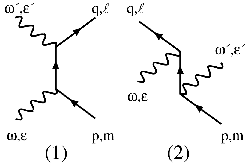
The sum in equation (1) is over the intermediate Landau states, labelled by quantum number $n$. The $F$ terms and phase factors are associated with the two different Feynman diagrams shown in Figure 1, and are listed explicitly in the Appendix. The $F$ terms of the second Feynman diagram can be obtained from those of the first diagram through the crossing-symmetry replacements

$$\omega\Leftrightarrow-\omega^{\prime},\ \ \ k\Leftrightarrow-k^{\prime},\ \ \beta\Leftrightarrow\beta^{\prime},\ \hbox{and}\ \varepsilon\Leftrightarrow\varepsilon^{\prime*}\quad.$$ (3)

For each Feynman diagram, each $F$ expression has a spin no-flip and a spin flip $F$ term associated with it, due to the spin degeneracy of the final states. Notation used in defining the $F$ terms and appearing elsewhere in this paper includes $\varepsilon$, which represents the photon polarization components defining two orthogonal linear polarization vectors as given in Daugherty & Bussard (1980):

$$\varepsilon^{\parallel} = -\cos\theta\cos\phi\hat{x}-\cos\theta\sin\phi\hat{y}+\sin\theta\hat{z},$$

$$\varepsilon_{\pm}^{\parallel} = \varepsilon_{x}^{\parallel}\pm i\varepsilon_{y}^{\parallel}=-\cos\theta e^{\pm i\phi},$$

$$\varepsilon_{z}^{\parallel} = \sin\theta,$$

$$\varepsilon^{\perp} = \sin\phi\hat{x}-\cos\phi\hat{y},$$

$$\varepsilon_{\pm}^{\perp} = \varepsilon_{x}^{\perp}\pm i\varepsilon_{y}^{\perp}=\mp ie^{\pm i\phi},$$

$$\varepsilon_{z}^{\perp} = 0$$

and the “vertex” functions, which in the notation of DH86 have the form

$$\Lambda_{\ell,m}(\beta)=(-i)^{G-S}\left({{{S!}\over{G!}}}\right)^{1/2}2^{-(G+S)/2}(\beta^{*})^{\ell}\beta^{m}\left({{{\left|\beta\right|^{2}}\over 2}}\right)^{-S}L_{S}^{G-S}\left({{{\left|\beta\right|^{2}}\over 2}}\right),$$ (5)

where

$$G=\max(\ell,m), \ S=\min(\ell,m),$$

$$\beta=-i{{(k_{x}+ik_{y})}\over{\sqrt{B}}}, \ \beta^{\prime}=i{{(k^{\prime}_{x}+ik^{\prime}_{y})}\over{\sqrt{B}}}$$

and $L^{a}_{n}(x)$ are the associated Laguerre polynomials.

3 SCATTERING OF RELATIVISTIC ELECTRONS

We consider in this study the particular problem of scattering of photons from relativistic electrons, common to a variety of astrophysical phenomena. Such relativistic scattering leads to considerable simplification of the algebra. In this section we develop expressions for scattering of ultra-relativistic electrons with $\gamma\gg 1$ moving parallel to the magnetic field lines. Generally, the photon may have any angle of incidence, $\psi_{i}$, in the laboratory frame with respect to the magnetic field. Due to the large $\gamma$’s, the laboratory angle, $\psi_{i}$, gets Lorentz contracted to $\theta=\psi_{i}/2\gamma\sim 0$ degrees in the electron rest frame. The magnetic, nonrelativistic Thomson cross section (Canuto, Lodenquai & Ruderman 1971, Blandford & Scharlemann 1976, and Herold 1979) consists of two parts dependent on the incident photon angle as shown in the expression

$$\sigma_{\rm Thomson}=\sigma_{\rm T}\left[{\sin^{2}\theta+{{\omega^{2}}\over 2}(1+\cos^{2}\theta)\left({{1\over{(\omega-B)^{2}}}+{1\over{(\omega+B)^{2}}}}\right)}\right].$$ (7)

Well below the resonance for angles, $\theta\ll\omega/B\ll 1$, corresponding to $\psi_{i}\ll 2\gamma\omega/B$ in the laboratory frame, the $\sin^{2}\theta$ term is smaller than the resonant term. In the case of isotropic incident photons in the laboratory frame (where $0<\psi_{i}<\pi$), this constraint requires $\omega\gg\pi B/2\gamma$, easily achieved with the large $\gamma$ of relativistic electrons considered throughout this paper. Under this assumption, the incident photon is parallel to the magnetic field lines and has no perpendicular momentum; hence

$$\theta = 0,$$

$$k_{\bot} = 0,$$

$$\varepsilon_{z} = 0,$$ (8)

$$\Phi_{1}=-\Phi_{2} = 0,$$

$$\beta = 0.$$

The coordinate system can be arbitrarily set so that the azimuthal angle, $\phi=0$. Since the incident photon is parallel to the z-axis, there is no component of the polarization vector, $\varepsilon_{z}$, along the z-axis, thereby, eliminating several terms in the $F$’s. The vertex functions associated with the incident photon become Kronecker delta functions, $\Lambda_{l,m}(0)=\delta_{lm}$. This has the advantage of eliminating the sum over the intermediate states as only certain specific states contribute depending on the final Landau state, $\ell$. The vertex functions associated with the scattered photon can be written in terms of a single function using the following recursion relations

$$\Lambda_{\ell-1,0}(\beta^{\prime}) = i{{\sqrt{2\ell}}\over{\beta^{\prime*}}}\Lambda_{\ell,0}(\beta^{\prime}),$$

$$\Lambda_{\ell,1}(\beta^{\prime}) = {{i\sqrt{2}}\over{\beta^{\prime*}}}\left({\ell-{{\left|\beta^{\prime}\right|^{2}}\over 2}}\right)\Lambda_{\ell,0}(\beta^{\prime}),$$

$$\Lambda_{\ell-1,1}(\beta^{\prime}) = -{{2\sqrt{\ell}}\over{(\beta^{\prime*})^{2}}}\left({\ell-1-{{\left|\beta^{\prime}\right|^{2}}\over 2}}\right)\Lambda_{\ell,0}(\beta^{\prime}),$$ (9)

$$\Lambda_{\ell+1,0}(\beta^{\prime}) = -i{{\beta^{\prime*}}\over{\sqrt{2(\ell+1)}}}\Lambda_{\ell,0}(\beta^{\prime}),$$

$$\Lambda_{\ell-2,0}(\beta^{\prime}) = -{{2\sqrt{\ell(\ell-1)}}\over{(\beta^{\prime*})^{2}}}\Lambda_{\ell,0}(\beta^{\prime}).$$

The $F$ terms associated with each Feynman diagram can then be rewritten, with the common vertex function $\Lambda_{l,0}(\beta^{\prime})$ being factored out of the scattering amplitudes to generate coefficients $G_{i}$ such that $G_{i}\Lambda_{\ell,0}(\beta^{\prime})=F_{n,i}^{(1)}+F_{n,i}^{(2)}$, where $i$ = flip and no-flip. Using the identity

$$\Bigl{|}{\Lambda_{\ell,0}(\beta^{\prime})}\Bigr{|}^{2}={{{\left|\beta^{\prime}\right|^{2\ell}}}\over{2^{\ell}\ell!}}={1\over{\ell!}}\left({{{\omega^{\prime 2}\sin^{2}\theta^{\prime}}\over{2B}}}\right)^{\ell},$$ (10)

the differential cross section can be expressed compactly as

$${{d\sigma_{\parallel,\perp}}\over{d\cos\theta^{\prime}}}={{3\sigma_{\rm T}}\over{16\pi}}{{\omega^{\prime 2}e^{-\omega^{\prime 2}\sin^{2}\theta^{\prime}/2B}}\over{\omega(2+\omega-\omega^{\prime})(\omega^{\prime}+\omega\omega^{\prime}(1-\cos\theta^{\prime})-\omega^{\prime 2}\sin^{2}\theta^{\prime})}}{1\over{\ell!}}\left({{{\omega^{\prime 2}\sin^{2}\theta^{\prime}}\over{2B}}}\right)^{\ell}\;{G_{\parallel,\perp}},$$ (11)

where

$$G_{\parallel}=\hat{G}_{no\,flip}^{\parallel}+\hat{G}_{flip}^{\parallel},\quad G_{\perp}=\hat{G}_{no\,flip}^{\perp}+\hat{G}_{flip}^{\perp},$$ (12)

and

$$\hat{G}_{no\,flip}^{||} = \int\limits_{0}^{2\pi}{\left|{G_{no\,flip}^{||,||}}\right|^{2}d\phi^{\prime}}=\int\limits_{0}^{2\pi}{\left|{G_{no\,flip}^{\bot,||}}\right|^{2}d\phi^{\prime}}$$

$$= 2\pi\left\{{\,\left[{(B_{1}+B_{3}+B_{7})\cos\theta^{\prime}-(B_{2}+B_{6})\sin\theta^{\prime}}\right]^{2}+\left[{B_{4}\cos\theta^{\prime}-B_{5}\sin\theta^{\prime}}\right]^{2}}\right\},$$

$$\hat{G}_{no\,flip}^{\bot} = \int\limits_{0}^{2\pi}{\left|{G_{no\,flip}^{||,\bot}}\right|^{2}d\phi^{\prime}}=\int\limits_{0}^{2\pi}{\left|{G_{no\,flip}^{\bot,\bot}}\right|^{2}d\phi^{\prime}}$$

$$= 2\pi\left\{{\,(B_{1}-B_{3}-B_{7})^{2}+B_{4}^{2}}\right\},$$

$$\hat{G}_{flip}^{||} = \int\limits_{0}^{2\pi}{\left|{G_{flip}^{||,||}}\right|^{2}d\phi^{\prime}}=\int\limits_{0}^{2\pi}{\left|{G_{flip}^{\bot,||}}\right|^{2}d\phi^{\prime}}$$

$$= 2\pi\left\{{\,\left[{(C_{1}+C_{3}+C_{7})\cos\theta^{\prime}-(C_{2}+C_{6})\sin\theta^{\prime}}\right]^{2}+\left[{C_{4}\cos\theta^{\prime}-C_{5}\sin\theta^{\prime}}\right]^{2}}\right\},$$

$$\hat{G}_{flip}^{\bot} = \int\limits_{0}^{2\pi}{\left|{G_{flip}^{||,\bot}}\right|^{2}d\phi^{\prime}}=\int\limits_{0}^{2\pi}{\left|{G_{flip}^{\bot,\bot}}\right|^{2}d\phi^{\prime}}$$

$$= 2\pi\left\{{\,(C_{1}-C_{3}-C_{7})^{2}+C_{4}^{2}}\right\}.$$

In these developments, the $\phi^{\prime}$ dependence and the imaginary terms are isolated in the polarization components and the phase exponentials, leading to elementary integrations over the azimuthal angle, $\phi^{\prime}$. The $B$ and $C$ terms have the following forms:

$$B_{1} = {{\left[{2\omega-\omega\omega^{\prime}(1-\cos\theta^{\prime})}\right]}\over{2(\omega-B)}},$$

$$B_{2} = -{{\left[{(\omega-\omega^{\prime}\cos\theta^{\prime})\left({2lB-\omega^{\prime 2}\sin^{2}\theta^{\prime}}\right)+2lB\omega}\right]}\over{2\omega^{\prime}\sin\theta^{\prime}(\omega-B)}},$$

$$B_{3} = {{lB\left({2lB-2B-\omega^{\prime 2}\sin^{2}\theta^{\prime}}\right)}\over{\omega^{\prime 2}\sin^{2}\theta^{\prime}(\omega-B)}},$$

$$B_{4} = -{{\left[{2\omega^{\prime}+\omega\omega^{\prime}(1-\cos\theta^{\prime})-\omega^{\prime 2}\sin^{2}\theta^{\prime}}\right]}\over{2\left[{\omega\omega^{\prime}(1-\cos\theta^{\prime})-\omega-B}\right]}},$$

$$B_{5} = -{{(\omega-\omega^{\prime}\cos\theta^{\prime})\omega^{\prime}\sin\theta^{\prime}}\over{2\left[{\omega\omega^{\prime}(1-\cos\theta^{\prime})-\omega-B}\right]}},$$

$$B_{6} = {{\ell B\cos\theta^{\prime}}\over{\sin\theta^{\prime}\left[{\omega\omega^{\prime}(1-\cos\theta^{\prime})-\omega+B}\right]}},$$

$$B_{7} = {{2\ell(\ell-1)B^{2}}\over{\omega^{\prime 2}\sin^{2}\theta^{\prime}\left[{\omega\omega^{\prime}(1-\cos\theta^{\prime})-\omega+B}\right]}},$$

$$C_{1} = \sqrt{2\ell B}{\omega\over{2(\omega-B)}},$$

$$C_{2} = -\sqrt{2lB}{{\left[{2\omega+2\omega^{2}-\omega\omega^{\prime}(1-\cos\theta^{\prime})-2lB+\omega^{\prime 2}\sin^{2}\theta^{\prime}}\right]}\over{2\omega^{\prime}\sin\theta^{\prime}(\omega-B)}},$$

$$C_{3} = \sqrt{2lB}{{\left({\omega-\omega^{\prime}\cos\theta^{\prime}}\right)\left({2lB-2B-\omega^{\prime 2}\sin^{2}\theta^{\prime}}\right)}\over{2\omega^{\prime 2}\sin^{2}\theta^{\prime}(\omega-B)}},$$

$$C_{4} = -\sqrt{2\ell B}{{\omega^{\prime}\cos\theta^{\prime}}\over{2\left[{\omega^{\prime}\omega(1-\cos\theta^{\prime})-\omega-B}\right]}},$$

$$C_{5} = \sqrt{2\ell B}{{\omega^{\prime}\sin\theta^{\prime}}\over{2\left[{\omega^{\prime}\omega(1-\cos\theta^{\prime})-\omega-B}\right]}},$$

$$C_{6} = -\sqrt{2\ell B}{{\left[{2\omega^{\prime}+\omega\omega^{\prime}(1-\cos\theta^{\prime})-\omega^{\prime 2}\sin^{2}\theta^{\prime}}\right]}\over{2\omega^{\prime}\sin\theta^{\prime}\left[{\omega^{\prime}\omega(1-\cos\theta^{\prime})-\omega+B}\right]}},$$

$$C_{7} = \sqrt{2\ell B}{{(l-1)B\left({\omega-\omega^{\prime}\cos\theta^{\prime}}\right)}\over{\omega^{\prime 2}\sin^{2}\theta^{\prime}\left[{\omega^{\prime}\omega(1-\cos\theta^{\prime})-\omega+B}\right]}}.$$

Since this combination of expressions for the differential cross section is for the particular case of scattering of relativistic electrons with an incident photon angle of zero degrees in the electron rest frame, the resulting scattering rates are simple and do not possess the sum over Bessel functions as in Bussard et al. (1986). While there are four different possibilities for the scattering of polarized photons, ($\parallel\rightarrow\parallel$, $\perp\rightarrow\parallel$, $\parallel\rightarrow\perp$, and $\perp\rightarrow\perp$), for this special case under consideration, the expressions for the $\parallel\rightarrow\parallel$, $\perp\rightarrow\parallel$ scattering have the same form, as well as those for the $\parallel\rightarrow\perp$, and $\perp\rightarrow\perp$ scattering, as indicated above, resulting in two polarization channels in which the scattering process will produce either parallel or perpendicular polarized photons.

Observe also that the differential cross section is dependent on the final Landau state, $\ell$. Hence, in order to derive the complete contribution, a sum must be performed over all the contributing Landau states. Since the energy of the scattered photon may be expressed as

$$\omega^{\prime}={{2(\omega-\ell B)}\over{1+\omega(1-\cos\theta^{\prime})+\left[{\left({1+\omega(1-\cos\theta^{\prime})}\right)^{2}-2(\omega-\ell B)\sin^{2}\theta^{\prime}}\right]^{1/2}}}\;\;,$$ (15)

where $\ell$ is the final Landau state of the scattered electron, each final state has an energy threshold of $\ell B$. Therefore, the maximum contributing Landau state quantum number, $\ell_{max}$, to the cross section is pinned to the photon energy in cyclotron units: $\omega/B-1<\ell_{max}<\omega/B$.

4 ANGLE-INTEGRATED CROSS SECTIONS

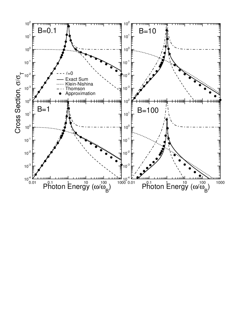
The differential cross section can be numerically integrated over $\theta^{\prime}$ using a Romberg integration scheme to obtain the energy dependent cross section. In Figure 2, we display the QED, exact angle-integrated cross section (solid curves) for the indicated magnetic fields, in units of $B_{\rm cr}$, as a function of the incident photon energy, $\omega/B$, in cyclotron energy units. We have averaged over the final spin of the electron and over the polarization of the scattered photon. For this particular case in the scattering of relativistic electrons, there is only one resonance occurring at the fundamental cyclotron resonance of $\omega_{B}=B$. We scale the photon energy by the cyclotron energy so that the resonance occurs at the same place independent of the magnetic field, $B$. For comparison, we also plot in the figures the nonrelativistic Thomson limit (dot-dashed curves) and the Klein-Nishina (dotted curves) predictions. The solid circles are the result of an approximation that is discussed later in section 6. For the exact calculation, we have summed over the all the contributing final Landau states.

Above the resonance, the exact cross section approaches the Klein-Nishina cross section. As expected for smaller fields, the convergence occurs at lower photon energies, as seen in the case of $B=0.1$. At this field strength, typical of radio pulsars, there are no significant deviations from the Thomson limit below the resonance and from the Klein-Nishina limit above the resonance. The main discrepancy occurs right above the resonance where the two limiting cases do not match the exact cross section. As the field strength increases, the exact cross section below the resonance drops significantly beneath the Thomson limit by over a factor of ten in the case of $B=100$ For scattering above the resonance at these high fields, there are deviations between the exact cross section and the Klein-Nishina cross section. However, as the energy increases, the exact cross section and the Klein-Nishina cross section appear to converge as seen in the cases of $B=0.1$ and $B=1$.

The trend as $B$ increases, evident in Figure 2, is for the magnitude of the cross section to drop at all energies, while the width of the resonance increases (for $B\geq 1$, when scaled in units of the cyclotron energy, this width actually declines). Since the resonance is formally divergent, the common practice (Xia et al. 1985, Daugherty & Harding 1989 and Dermer 1990) is to truncate it at $\omega=B$ by introducing a finite width $\Gamma$ equal to the cyclotron decay width (inverse lifetime) for the $\ell=1\rightarrow 0$ transitions, corresponding to decay of an excited intermediate electron state. The procedure is to replace the resonant $(\omega-B)^{2}$ denominator (e.g. see equation (LABEL:eq:dsig_leq0_approx) below) by $\left[(w-B)^{2}+G^{2}/4\right]$. In the $B\ll 1$ regime, the cyclotron decay width assumes the well-known result $\Gamma=4\alpha B^{2}/3$ in dimensionless units. When $B\gg 1$, Latal (1986) deduced that $\Gamma$ is proportional to $B^{1/2}$, a dependence that can be inferred from the exact decay widths enunciated in equation (17) of Herold, Ruder & Wunner (1982) by noting that the angular distribution of radiation in cyclotron transitions is still quasi-isotropic (and not strongly beamed) for highly-supercritical fields. When substituted into the Lorentz profile prescription for truncating the resonance, these widths lead to the areas under the resonance (i.e. when integrating over $\omega$) being independent of $B$ in the magnetic Thomson regime of $B\ll 1$, and scaling as $B^{1/2}$ when $B\gg 1$; these results can be deduced using the $\ell=0$ approximation derived in equation (LABEL:eq:dsig_leq0_approx).

This area is an approximate measure of the importance of resonant Compton scattering for a particular situation. To see this, note that astrophysical problems generally have a broad energy distribution of beamed relativistic electrons interacting with not-so-highly-beamed low energy (soft) photons, so that a particular electron energy and soft photon angle (with respect to $B$) determines the value of $\omega$ in the electron rest frame. Summing over the electron energies and incoming photon angles amounts to a weighted integration of the area under the cross section. The weighting function is usually not very sensitive to $\omega$, so that the area under the curves gives a representative indication of the strength of resonant (as opposed to non-resonant) scattering provided the resonance is not too broad. Hence, it can be inferred that the resonant process is more important in supercritical fields than when $B\ll 1$. This conclusion stands even when it is noted that the magnetic Compton resonance is not truly cyclotronic in nature: the contribution of the $\ell=1$ transition to the right wing of the resonance plus the spread of parallel momenta introduce non-Lorentzian distortions to the resonance profile.

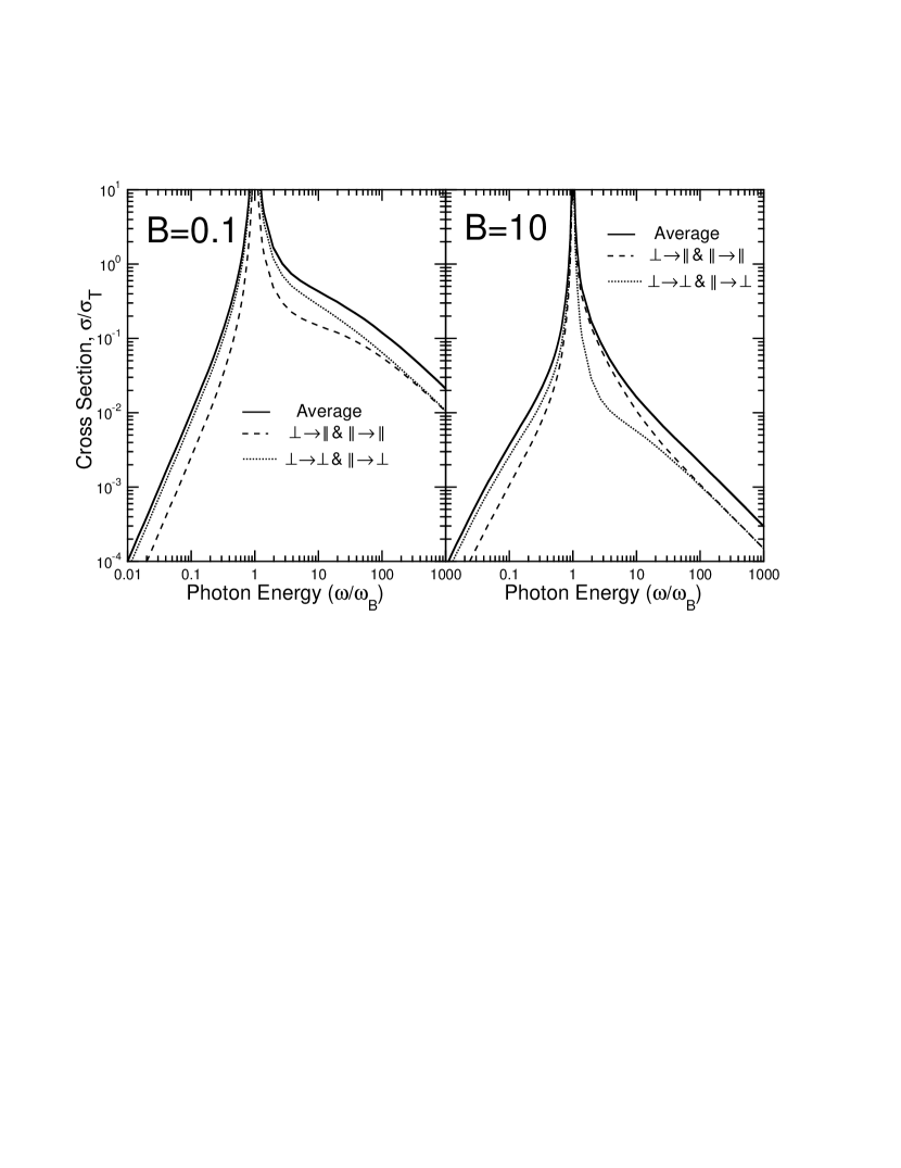
The photon polarization-dependent cross sections can also be easily obtained for the given integration of the $G$ terms shown above. In Figure 3, we present the QED Compton scattering cross section as a function of energy for magnetic fields of 0.1 and 10 times $B_{\rm cr}$. As mentioned earlier, for this particular case of scattering of relativistic electrons, there are two polarization scattering channels, in which the scattering leads to photons with parallel polarization (dashed curve) and with perpendicular polarization (dotted curve). The total cross section is shown as a solid curve. In the $B=10$ case, above the resonance, the scattering process preferably produces photons with parallel polarization, whereas below the resonance, the channel producing perpendicularly polarized photons dominates. This behavior, where perpendicular-polarized scattered photons dominate below the resonance and parallel-polarized scattered photons dominate above the resonance, is characteristic of the magnetic-relativistic cross section. In the nonrelativistic case, the perpendicular polarization channel will be three times larger than the parallel polarization channel, but has the same shape at all photon energies, as observed from equation (LABEL:eq:dsig_leq0_approx) letting $\omega^{\prime}\rightarrow\omega$ and integrating over $\cos\theta^{\prime}$. As can be seen in the Figure 3 for the $B=0.1$ case, $\parallel$-polarization in the QED cross section dominates at low fields, thus the switching to $\perp$-polarization dominance at high fields is a relativistic effect. In the Klein-Nishina scattering there is no magnetic field and the initial photon polarization is important in determining the final photon polarization. In this case, there are three channels, $\parallel\rightarrow\parallel$, $\perp\rightarrow\perp$, and two degenerate switching channels $\perp\rightarrow\parallel$ and $\parallel\rightarrow\perp$. In the Klein-Nishina regime, right above the resonance, the $\perp\rightarrow\perp$ channel dominates over the $\parallel\rightarrow\parallel$ channel and the switching channels $\perp\rightarrow\parallel$ and $\parallel\rightarrow\perp$ which have the smallest contribution. Far above the resonance at high photon energies, the cross sections for the three channels merge as in the magnetic cross section in Figure 3.

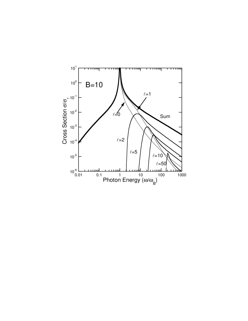
In Figure 4, we show the contributions of the indicated final Landau states to the total cross section for the indicated field strength of 10 times $B_{\rm cr}$. The total cross section, represented by a thick-solid curve, is a result of summing over all contributing Landau states. Below the resonance, only the $\ell=0$ final state contributes (dotted curve) to the cross section due to the previously mentioned threshold associated with each $\ell$. The curve associated with $\ell=1$, having a similar shape as the $\ell=0$ curve, is plotted also as a dotted curve. The light solid curves represent a select group of the indicated higher final Landau states. As the photon energy increases, higher $\ell$ states may contribute more significantly than lower ones. For example, above a photon energy of 50, the $\ell=10$ state contributes more to the overall cross section than the $\ell=0$ or 1 states (dotted curves). Clearly for scattering above the resonance, many final states must be included for computational accuracy.

As mentioned earlier, the cross section of DH86 was derived using Johnson-Lippmann (JL) electron wavefunctions which do not correctly describe the spin-dependence of the S-matrix elements, but produce correct spin-averaged S-matrix elements. Thus, we have averaged over the initial and summed over final electron spin states in the expressions we derived. However, there is still a small error in the JL cross section at and above the cyclotron resonance, due to the spin-dependence of the intermediate states. This error is negligible for $B<0.1$ but grows with $B$ for $B>0.1$. We have evaluated this error through a numerical comparison of the JL cross section of DH86, derived in this paper that neglect the decay width of the intermediate states, with the cross section derived by Sina (1996) who used Sokolov-Ternov (ST) wavefunctions. For the case of the scattering of relativistic electrons with $\psi_{i}=0$, the two spin-averaged cross sections agree below the cyclotron energy, $B$, but do not quite agree for $\omega\geq B$. We find that for $B=0.1$, there is a small error of 0.01% at $\omega=B$ in the spin-averaged cross section and for $B=10$, there is a somewhat larger error of 0.4% at $\omega=B$. The increasing error with increasing magnetic field is due to the intermediate states having non-zero momentum which increases the difference between JL and ST cross sections at higher $B$ fields. Thus the simplified expressions derived in this paper are accurate in their regions of validity. Furthermore, the cyclotron energy is high enough in supercritical fields that scattering above the resonance is less important than it is in subcritical fields. We plan to use the ST cross section in future derivation of simplified expressions for the scattering cross section above the cyclotron resonance.

5 SCATTERING TO $\ell=0$ FINAL STATES - BELOW THE RESONANCE

Due to the presence of the resonance in the cross section, the scattering process will try to select out resonant scattering, if the geometry and the kinematics permit. As the magnetic field increases, the photon energy, in the electron rest frame, required for resonant scattering (i.e., $\omega=B$) increases. If the source of photons is limited by blackbody temperatures and the field strength is large, the scattering will predominately occur much below the resonance. The cross sections, described here, are in the rest frame of the electron. If the electron is moving, the Lorentz-transformed photon energy in the electron rest frame is given by

$$E_{rest}=E_{lab}\gamma(1-\beta\cos\psi_{i}),$$ (16)

where $E_{rest}$ and $E_{lab}$ are the energies of the photon in the rest and laboratory frames, respectively, and $\psi_{i}$ is the laboratory angle of the photon with respect to the electron direction. For small angles $\psi_{i}\sim 0$, where the photon is moving in the same direction as the electron, the photon energy is red shifted, $E_{rest}\sim E_{lab}/(2\gamma)$. For large angles $\psi_{i}\sim\pi$, where the photon and electron are colliding head on, the photon energy is blue shifted, $E_{rest}\sim 2\gamma E_{lab}$. For perpendicular scattering, the photon energy is also blue shifted, $E_{rest}\sim\gamma E_{lab}$. In general, when the incident angle, $\psi_{i}>\sqrt{2/\gamma}$, the photon energy will be blue shifted. For relativistic electrons, the geometry of the interaction becomes important in determining whether the scattering takes place above or below the resonance.

If the scattering occurs below the resonance, the only contribution to the cross section is from the $\ell=0$ final state, since the final Landau state, $\ell$, state has an energy threshold of $\ell B$. Using the following identity valid for $\ell=0$,

$$\omega^{\prime 2}\sin^{2}\theta^{\prime}=2\omega^{\prime}-2\omega-\omega\omega^{\prime}(1-\cos\theta^{\prime}),$$ (17)

in the denominator of equation (11), the expression for the exact, QED, cross section of the $\ell=0$ final state has the following form

$${{d\sigma}\over{d\cos\theta^{\prime}}}={{3\sigma_{\rm T}}\over{16\pi}}{{\omega^{\prime 2}}\over{\omega(2+\omega-\omega^{\prime})(\xi-\omega^{\prime})}}e^{-\omega^{\prime 2}\sin^{2}\theta^{\prime}/2B}\;G\quad,$$ (18)

where

$$\xi=2\omega-\omega\omega^{\prime}(1-\cos\theta^{\prime}).$$ (19)

All the $C$ terms associated with the spin flip drop out for the $\ell=0$ case, in addition the $B_{3}$, $B_{6}$ and $B_{7}$ terms are zero. The remaining nonzero $B$ terms simplify to the following

$$B_{1} = {\xi\over{2(\omega-B)}},$$

$$B_{2} = {\eta\over{2(\omega-B)}},$$

$$B_{4} = -{{-\xi}\over{2(\omega-\xi-B)}},$$ (20)

$$B_{5} = -{\eta\over{2(\omega-\xi-B)}},$$

where

$$\eta=(\omega-\omega^{\prime}\cos\theta^{\prime})\omega^{\prime}\sin\theta^{\prime}.$$ (21)

The exact polarization-dependent and averaged cross sections for $\ell=0$ can be expressed as

$${{d\sigma^{||\to||}}\over{d\cos\theta^{\prime}}} = {{d\sigma^{\perp\to||}}\over{d\cos\theta^{\prime}}}={{3\sigma_{\rm T}}\over{32}}{{\omega^{\prime 2}e^{-\omega^{\prime 2}\sin^{2}\theta^{\prime}/2B}}\over{\omega(2+\omega-\omega^{\prime})(\xi-\omega^{\prime})}}$$

$$\times\left\{{\left({\xi\cos\theta^{\prime}-\eta\sin\theta^{\prime}}\right)^{2}\left[{{1\over{(\omega-B)^{2}}}+{1\over{(\omega-\xi-B)^{2}}}}\right]}\right\},$$

$${{d\sigma^{||\to\perp}}\over{d\cos\theta^{\prime}}} = {{d\sigma^{\perp\to\perp}}\over{d\cos\theta^{\prime}}}={{3\sigma_{\rm T}}\over{32}}{{\omega^{\prime 2}e^{-\omega^{\prime 2}\sin^{2}\theta^{\prime}/2B}}\over{\omega(2+\omega-\omega^{\prime})(\xi-\omega^{\prime})}}$$ (23)

$$\times\left\{{\xi^{2}\left[{{1\over{(\omega-B)^{2}}}+{1\over{(\omega-\xi-B)^{2}}}}\right]}\right\},$$

$${{d\sigma^{ave}}\over{d\cos\theta^{\prime}}} = {{3\sigma_{\rm T}}\over{32}}{{\omega^{\prime 2}e^{-\omega^{\prime 2}\sin^{2}\theta^{\prime}/2B}}\over{\omega(2+\omega-\omega^{\prime})(\xi-\omega^{\prime})}}$$

$$\times\left\{{\left[{\left({\xi\cos\theta^{\prime}-\eta\sin\theta^{\prime}}\right)^{2}+\xi^{2}}\right]\left[{{1\over{(\omega-B)^{2}}}+{1\over{(\omega-\xi-B)^{2}}}}\right]}\right\}.$$

The average cross section is obtained by summing over the final and averaging over the initial photon polarizations.

6 APPROXIMATING THE $\ell=0$ FINAL STATES

An approximation to the exact $\ell=0$ differential cross section can be given by assuming that the scattering is significantly below the resonance, where $\omega<B$, and also $\omega<1$. We make this approximation by keeping only terms to first order in $\omega$ and $\omega^{\prime}$ in the two forms,

$$\xi = 2\omega-\omega\omega^{\prime}(1-\cos\theta^{\prime})\to 2\omega,$$

$$\eta = (\omega-\omega^{\prime}\cos\theta^{\prime})\omega^{\prime}\sin\theta^{\prime}\to 0.$$ (24)

This leads to the following approximate expressions

$${{d\sigma^{||\to||}}\over{d\cos\theta^{\prime}}} \approx {{d\sigma^{\perp\to||}}\over{d\cos\theta^{\prime}}}={{3\sigma_{\rm T}}\over 8}{{\omega\omega^{\prime 2}\cos^{2}\theta^{\prime}}\over{(2\omega-\omega^{\prime})}}\left[{{1\over{(\omega-B)^{2}}}+{1\over{(\omega+B)^{2}}}}\right],$$

$${{d\sigma^{||\to\perp}}\over{d\cos\theta^{\prime}}} \approx {{d\sigma^{\perp\to\perp}}\over{d\cos\theta^{\prime}}}={{3\sigma_{\rm T}}\over 8}{{\omega\omega^{\prime 2}}\over{(2\omega-\omega^{\prime})}}\left[{{1\over{(\omega-B)^{2}}}+{1\over{(\omega+B)^{2}}}}\right],$$

$${{d\sigma^{ave}}\over{d\cos\theta^{\prime}}} \approx {{3\sigma_{\rm T}}\over 8}{{\omega\omega^{\prime 2}(1+\cos^{2}\theta^{\prime})}\over{(2\omega-\omega^{\prime})}}\left[{{1\over{(\omega-B)^{2}}}+{1\over{(\omega+B)^{2}}}}\right].$$

The nonrelativistic approximation would further lead to $\omega^{\prime}=\omega$, resulting in the nonrelativistic expressions found in Herold (1979).

These expressions, while much simpler than the previous ones, are still complex due to the functional form of $\omega^{\prime}$, having an angular dependence in its square root. Yet they are manageable and can be integrated over $\cos\theta^{\prime}$. After careful algebra, integration over $\cos\theta^{\prime}$ yields the following polarization-dependent and averaged, approximate cross sections

$$\sigma^{||\to||} = \sigma^{\perp\to||}={{3\sigma_{\rm T}}\over{16}}\left\{{g(\omega)-h(\omega)}\right\}\left[{{1\over{(\omega-B)^{2}}}+{1\over{(\omega+B)^{2}}}}\right],$$

$$\sigma^{||\to\perp} = \sigma^{\perp\to\perp}={{3\sigma_{\rm T}}\over{16}}\left\{{f(\omega)-2\omega h(\omega)}\right\}\left[{{1\over{(\omega-B)^{2}}}+{1\over{(\omega+B)^{2}}}}\right],$$ (26)

$$\sigma^{ave} = {{3\sigma_{\rm T}}\over{16}}\left\{{g(\omega)+f(\omega)-(1+2\omega)h(\omega)}\right\}\left[{{1\over{(\omega-B)^{2}}}+{1\over{(\omega+B)^{2}}}}\right].$$

where

$$g(\omega) = {{\omega^{2}(3+2\omega)+2\omega}\over{\sqrt{\omega(2+\omega)}}}\ln\left({1+\omega-\sqrt{\omega(2+\omega)}}\right)+{\omega\over 2}\ln(1+4\omega)$$

$$+\omega(1+2\omega)\ln(1+2\omega)+2\omega,$$

$$f(\omega) = -\omega^{2}\ln(1+4\omega)+\omega(1+2\omega)\ln(1+2\omega),$$ (27)

$$h(\omega) = \left\{\begin{array}[]{ll}{{\omega^{2}}\over{\sqrt{\omega(2-\omega)}}}\tan^{-1}\left({{{\sqrt{\omega(2-\omega)}}\over{1+\omega}}}\right),&\mbox{for $\omega<2$,}\\ {{\omega^{2}}\over{2\sqrt{\omega(\omega-2)}}}\ln\left({{{\left({1+\omega+\sqrt{\omega(\omega-2)}}\right)^{2}}\over{1+4\omega}}}\right),&\mbox{for $\omega>2$.}\end{array}\right.$$ (30)

While one might expect $h(\omega)$ to become imaginary when $\omega>2$, given the $(2-\omega)$ factor in the square-root terms in first expression for $h(\omega)$, the expression is completely general and remains real even when $\omega>2$. For the purpose of numerical calculations in a computer code, we introduce this second expression for $h(\omega)$ that can be coded using a natural logarithm when $\omega>2$.

Back in Figure 2, the solid circles represent the polarization-averaged cross section obtained from the above analytical approximation. The approximation is valid in the region below $\omega<1$ corresponding to $\omega/B<1/B$ along the photon energy axis in Figure 2. In this region, it agrees very well with the exact $\ell=0$ cross section. Above the region of validity, the approximation over estimates the exact $\ell=0$ cross section. However, the approximation does surprisingly well, when compared to the exact cross section, extrapolating above the region of validity. While the analytical approximation is a result of integrating the approximation to the exact $\ell=0$ differential cross section, it remains close to the total cross section at high $\omega$ above the resonance $(\omega>B)$ even for high field strengths.

7 ANGULAR DISTRIBUTIONS

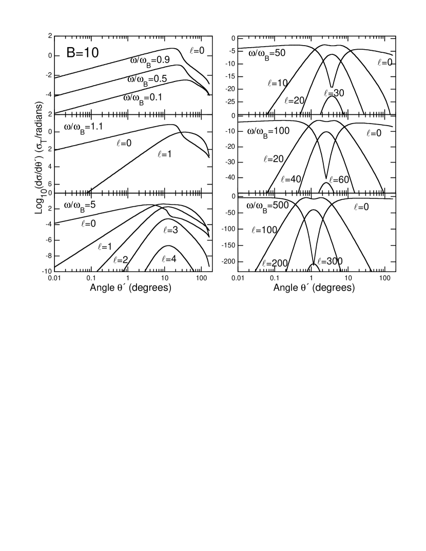
We present in Figure 5, the differential cross section, $d\sigma/d\theta^{\prime}$, for a magnetic field of $B=10B_{\rm cr}$. In order to understand best the behavior of the angular distributions, we have plotted the differential cross section as a function of the logarithm of the scattered angle, $\theta^{\prime}$, of the photon in the electron rest frame. We sample the angular distributions beginning below the resonance, where only the $\ell=0$ final Landau state contributes, to high above the resonance where many Landau states contribute up to the threshold $\ell_{max}$: $\omega/B-1<\ell_{max}<\omega/B$. The incident photon energies for each panel are indicated in units of the cyclotron energy, $\omega_{B}=B$. Also indicated are the final Landau states of the calculated angular distributions. As expected, the $\ell=0$ contribution is strong for all photon energies. As the photon energy increases high above the resonance (right panels of the figure), the angular distribution of the $\ell=0$ state reveals a dip at an energy-dependent angle in the forward direction. This dip is very steep, as indicated by the number of decades the distribution drops before approaching its minimum. Care must be exercised in this region, as one integrates the angular distributions. As the final Landau state increases, the angular distributions become more gaussian shaped, peaking at the same angle for a given photon energy as the minimum in the $\ell=0$ state. Above the resonance, the angular distributions evolve smoothly from a sharp minimum at low Landau states to a maximum at higher Landau states. Both the minima and maxima occur at invariably the same angle, $\theta_{o}$. This behavior is due to the functional form of the following factor in the differential cross section

$$f(\omega,\theta^{\prime})={1\over{\ell!}}\left({{{\omega^{\prime 2}\sin^{2}\theta^{\prime}}\over{2B}}}\right)^{\ell}\exp\Biggl{\{}{-{{\omega^{\prime 2}\sin^{2}\theta^{\prime}}\over{2B}}}\Biggr{\}},$$ (31)

which controls the angular dependence of the differential cross section, $d\sigma/d\cos\theta^{\prime}$. The first part of this function arises from the vertex functions mentioned earlier in equation (10). The first derivative with respect to $\theta^{\prime}$ of this function goes to zero an angle, $\theta_{o}$, given by

$$\theta_{o}=\tan^{-1}\left({{{\sqrt{1+2\omega}}\over\omega}}\right),$$ (32)

independent of $\ell$. Since $f(\omega,\theta^{\prime})$ is only part of the overall differential cross section, this expression for $\theta_{o}$ is approximate. Yet, it predicts very well the angle at which the angular distributions experience minima and maxima with increasing Landau states. The scattered photon energy, $\omega_{o}^{\prime}$, at which this peak in the angular distribution occurs is given by

$$\omega^{\prime}_{o}={{1+\omega}\over{1+2\omega}}\left({1+2\omega-\sqrt{(1+2\omega)(1+2\ell B)}}\right).$$ (33)

The Landau state, $\ell_{s}$, at which the angular distribution evolves from a minimum to a maximum at a given photon energy, $\omega$, occurs when the second derivative of the above function, $f(\omega,\theta^{\prime})$, with respect to $\theta^{\prime}$ is equal to zero and is given by the expression

$$\ell_{s}={{\omega^{2}}\over{2B(1+2\omega)}}.$$ (34)

The energy of scattered photon at $\ell_{s}$ and at $\theta_{o}$ has the simple form

$$\omega^{\prime}_{s}={{(1+\omega)\omega}\over{1+2\omega}}.$$ (35)

These expressions have served to guide the design of the algorithm that numerically integrates the angular distributions to obtain the integrated cross sections shown in Figure 2. For Landau states below, $\ell_{s}$, the angular distributions manifest the steep drop at $\theta_{o}$, therefore we integrate the angular distribution in two parts from $\theta=0$ to $\theta_{o}$ and from $\theta_{o}$ to $\pi$. When the Landau state is above, $\ell$s, the angular distributions are gaussian-shaped, and we integrate from $\theta=0$ to $\pi$.

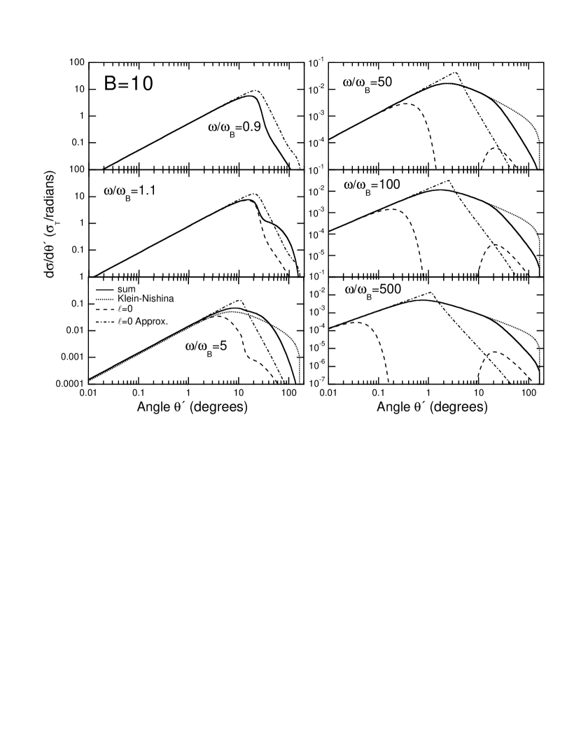
The peak in the total angular distribution will also occur very near this angle $\theta_{o}$ as seen in Figure 6. Here we present the total angular distributions summed over all the contributing final Landau states represented by the solid curves. The dashed curves show the angular distribution for the $\ell=0$ state. The approximation to the exact $\ell=0$ differential cross section given in equation (LABEL:eq:dsig_leq0_approx) (averaged) is plotted as dot-dashed curves. Comparing the exact-summed angular distributions (solid curves) to the approximate distributions (dot-dashed) in Figure 6, one can see in Figure 2 that the approximation falls below the integrated cross sections because there is a deficiency in the approximation at large angles. As expected, the $\ell=0$ state is the dominant contribution to the angular distribution at photon energies below and right above the resonance. As the photon energy increases well beyond the resonance, the $\ell=0$ state contributes less significantly and higher Landau states become increasingly important contributors. Although the strength of large Landau states decreases rapidly as shown in Figure 5, they are numerous and contribute significantly when summed to obtain the overall angular distributions shown in Figure 6. The contribution of these higher Landau states occurs near $\theta_{o}$, where the total angular distributions peak. It is at $\theta_{o}$ where minima occur in the angular distributions of final states of $\ell<\ell_{s}$. Yet the approximation to the $\ell=0$ final Landau state peaks at approximately the angle $\theta_{o}$. The angular distributions of the exact, the Klein-Nishina, and the $\ell=0$ approximate cross sections all peak where $\omega^{\prime}=\omega\ ({\rm at\ }\theta=\theta_{o})$. This is a result of the fact that the approximate angular distribution is governed by the kinematics. The scattered angle, $\theta^{\prime}$, is small at $\theta_{o}$, and the term $2(\omega-\ell B)\sin^{2}\theta^{\prime}$ in the denominator of equation (15) is also small resulting in an expression very similar to the Klein-Nishina kinematics. At scattering angles below $\theta_{o}$, there is significant agreement between the exact and Klein-Nishina angular distributions. The small-angle, low recoil scatterings, where one would expect all to agree because of similar kinematics, does not probe the effects of the field.

Differences are seen at large angle, large recoil scattering, where the geometry of the magnetic scattering is impacted by Landau excitations. High above the resonance, magnetic effects become manifested in the backward direction. Comparisons with the Klein-Nishina angular distributions for large photon energies, suggest that at backward angles the Klein-Nishina cross section over estimates the exact, summed, angular distributions beyond an angle of about 30 degrees. At these backward angles, Landau states larger than zero contribute significantly. While the term $2(\omega-\ell B)\sin^{2}\theta^{\prime}$ might be small at these angles, the $\ell B$ term in the numerator of $\omega^{\prime}$ in equation (15) becomes more important for larger $\ell$’s, and $\omega^{\prime}$ is significantly less than $\omega$, while $\omega^{\prime}$ in the Klein-Nishina kinematics remains close to $\omega$.

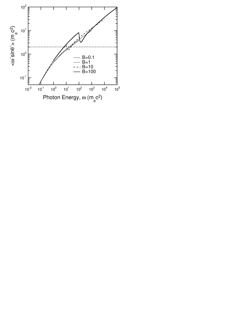
A quantity of interest in polar cap cascade models of highly magnetized gamma-ray pulsars is the mean value of the product $\omega^{\prime}\sin\theta^{\prime}$ achieved in resonant Compton scatterings. This product is a Lorentz invariant in transformations along the field lines, and represents the photon energy in the frame of reference where the upscattered photons move orthogonally to the local field. Hence, in conjunction with the value of $B$, this product principally controls the strength of strong-field photon attenuation processes such as pair creation $\gamma\rightarrow e^{+}e^{-}$ and photon splitting $\gamma\rightarrow\gamma\gamma$ . The mean value of $\omega^{\prime}\sin\theta^{\prime}$ in scatterings is therefore extremely informative for pulsar cascade modelers, and accordingly is plotted as a function of incident photon energy for different $B$ in Figure 7. The average was formed by weighting the differential cross sections such as those in Figure 5 with $\omega^{\prime}\sin\theta^{\prime}$ using equation (15), summing over quantum numbers $\ell$ and integrating over $\theta^{\prime}$, and then dividing by the total cross section (see Figure 2). The resulting curves exhibit a generally increasing function of $\omega$, with structure at the cyclotron resonances that becomes prominent in critical and supercritical fields due to the enhanced importance of $\ell>0$ (excited final state) scatterings above the fundamental; for a given $\theta^{\prime}$, higher $\ell$ values imply lower final photon energies $\omega^{\prime}$ (see equation [15]). The most salient property of Figure 7 is that the criterion for the scattered photons to generally rise above pair threshold is largely insensitive to the value of $B$, and is contingent upon the initial photon energy exceeding about 5-10 MeV in the electron rest frame.

Other general properties of $\left\langle\omega^{\prime}\sin\theta^{\prime}\right\rangle$ in Figure 7 can be understood as follows. Obviously there is naturally no expectation that the behavior of Figure 7 at low $B$ should mimic the non-magnetic scattering average at or below the cyclotron fundamental, because the total cross section does not approach the field-free Thomson limit when $\omega\ll B$ (see Figure 2). In fact, contrary to such intuition, at energies well below the cyclotron fundamental, $\left\langle\omega^{\prime}\sin\theta^{\prime}\right\rangle$ asymptotically approaches $15\pi\omega/64$ independent of $B$, derivable from the first line of equation (LABEL:eq:dsig_leq0_approx), a limit identical to the non-magnetic Thomson average. This ensues since, while the magnetic cross section has a different magnitude from the Thomson one, it possesses the same angular dependence (e.g. see equation (7.1b) of Rybicki & Lightman 1979), and $\omega^{\prime}\rightarrow\omega$ in this limit, independent of $B$. Departures from this low energy asymptote arise when $B\sim 1$. The analysis of the $\omega\gg B$ case is less trivial. Since the Klein-Nishina cross section is reproduced in sub-critical fields (e.g. see Figure 2), it might be anticipated that the Klein-Nishina $\left\langle\omega^{\prime}\sin\theta^{\prime}\right\rangle_{\rm KN}$ might result. This is realized, more or less, with the $B=0.1$ curve in Figure 7, which, if extrapolated, asymptotically approximates the non-magnetic Klein-Nishina average of

$$\left\langle{\omega^{\prime}\sin\theta^{\prime}}\right\rangle_{\rm KN}\mathrel{\mathop{\kern 0.0pt\longrightarrow}\limits_{\omega\gg B}}{{9\pi}\over 8}{{\sqrt{2\omega}}\over{2\ln(2\omega)+1}}$$ (36)

when $\omega\gg 10^{3}$. For higher $B$, deviations from pure Klein-Nishina behavior are more apparent, though the approximately $\omega^{1/2}$ dependence of $\left\langle\omega^{\prime}\sin\theta^{\prime}\right\rangle$ is generally maintained. The peak contribution to the cross section arises at scattered angles $\theta^{\prime}\approx 1/\omega^{1/2}$ when $\omega\gg 1$, as can be seen from equation (33), a consequence of kinematic constraints imposed by equation (15). In fact, this dependence of $\theta^{\prime}$ is similar to that for non-magnetic Klein-Nishina scattering, which possess similar (though not identical) kinematic restrictions. Furthermore, $\left\langle\theta^{\prime}\right\rangle$ is proportional to $\omega$ in this regime (for example, see equations (33) and (35)), a dependence borne out by the Klein-Nishina cross section, though the constants of proportionality differ, and indeed are a weakly increasing function of $B$ in the magnetic case here. Hence, in summary, the quantum kinematics of magnetic Compton scattering are qualitatively similar to those of Klein-Nishina scattering, and control the behavior of $\left\langle\omega^{\prime}\sin\theta^{\prime}\right\rangle$ when $\omega\gg B$ and concomitant deviations from the non-magnetic case.

8 DISCUSSION

In this paper, we have extended the work of DH86 by exploring the regime of super-critical fields and by providing simplified and explicitly real expressions for the exact differential cross section for Compton scattering in the presence of strong magnetic fields. We have derived simple analytic approximations for both the differential and total cross sections, in the special case of scattering by highly relativistic electrons, important to a variety of astrophysical sources. These results will be very useful in studying the effects of Compton scattering in the ultra-strong magnetic fields believed to be present near stellar surfaces of SGRs and AXPs. They also provide much more accurate expressions for modeling Compton scattering in the fields, $B>0.1$, of many pulsars. From the comparison of the exact, angle-integrated cross section with the limiting cases of the non-relativistic Thomson and the Klein-Nishina cross sections (used in neutron star applications throughout the literature) depicted in Figure 2, we can draw the following conclusions about scattering in increasing high fields: (i) below the resonance, the exact cross section is depressed below the magnetic Thomson cross section (when $\omega\geq m_{e}c^{2}$) differing by an order of magnitude or more for fields $B>10$; (ii) at the resonance, the exact cross section is dramatically reduced below the Thomson cross section, but the width of the resonance increases; (iii) far above the resonance, the exact cross section approaches the Klein-Nishina cross section, as expected for large photon energies, with the energy where the two merge an increasing function of $B$. The overall effect of the strong fields is to lower the cross section at all incident photon energies $\omega\geq m_{e}c^{2}$, decreasing the electron scattering opacity.

Focusing on large photon energies above the resonance, the magnetic field has a smaller perturbation on the interaction than around the resonance and below, and the exact cross section tends toward the Klein-Nishina limit, a feature that is seen in Figure 2 for $B\leq 10$. However, the analytical demonstration that these two cross sections approach each other in this high energy domain requires an approximation to the sum over many Landau states of the scattered electron and will be treated in a later paper. By inspection of the angular distributions in Figure 6, one can see that the disagreement between the exact cross section and the Klein-Nishina cross section occurs for moderate to extreme backward scattering, where the interaction probes the dominant effects of the magnetic field. It is also important to note that as the photon energy increases, the number of final Landau states contributing to the overall cross section increases dramatically, as seen in Figure 4, and as expected from the $\ell<\omega/B$ kinematic constraint. Care must be exercised in adding the contributions, as the numerical value of the cross section becomes very small for large Landau states.

From Figure 2 it is clear that even in relatively low fields $(B\approx 0.1)$, neither the magnetic Thompson nor the Klein-Nishina cross sections provides an adequate approximation to the exact cross section in a region right above the resonance, making a better representation of the exact cross section important for astrophysical models. Since the $\ell=0$ scattering provides the sole contribution to the cross section below the resonance, we were motivated to use it as a basis for developing an analytic approximation that is strictly only valid for $\omega\ll 1$ and $B\ll 1$. However, satisfyingly, the analytic approximation to the $\ell=0$ angle-integrated cross section can be extrapolated to $\omega\gg 1$ domains, and is able to represent the exact cross section quite well even at super-critical fields $(B\leq 10)$. This approximation indeed provides a smooth match to the exact cross section below the resonance, through the resonance and then above it where the Klein-Nishina-like reductions take over.

Use of the more accurate numerical results or approximate expressions that we have given here for resonant scattering will generally diminish the effects attributed to resonant Compton scattering in astrophysical models that use a non-relativistic treatment. This is because the non-relativistic cross section over-estimates the exact cross section when extrapolated to the domains (i.e. $\omega\geq 1,\ B\geq 1$) where relativistic effects are important or critical. Thus, we expect that the conditions for scattering to be significant in polar cap acceleration models will be more restricted: i.e., somewhat higher magnetic field strengths and soft photon densities will be required, than previously asserted, for Compton scattering to dominate over curvature radiation in the energy loss and pair production by primary particles (Sturner 1995, Harding & Muslimov 1998).

The cross section for Compton scattering is highly dependent on the photon polarization. Incident photons with either parallel or perpendicular polarization may switch polarization modes in a scattering. The calculations of this paper, as seen in Figure 3, show that the polarization-switching properties below the resonance are the same for the non-relativistic $(B\leq 1)$ and relativistic cases (i.e. more photons are scattered into the perpendicular mode). However for $B\geq 1$, the polarization-mode switching reverses above the resonance, so that scattering to the parallel mode is dominant. Such behavior contrasts that of the non-relativistic limit, where photons of perpendicular polarization are predominantly produced at all energies. In the case of the Klein-Nishina scattering where there is no magnetic field, the initial polarizations do matter in determining the final polarization resulting in three polarization channels, described earlier. Here too, the dominance of photons scattered to perpendicular polarization is manifested in the relativistic, non-magnetic Klein-Nishina case.

The polarization dependence of the scattering cross section in high fields will have significant implications for other polarization-dependent mechanisms such as pair production and, especially, photon splitting. As Baring & Harding (1998) noted, photon splitting could dominate pair production at supra-critical magnetic fields, thereby suppressing pair creation and possibly accounting for the radio quiescence of SGRs and AXPs. However, kinematic selection rules (Adler 1971; Shabad 1975) allow only one splitting mode to operate in the limit of weak dispersion, that in which photons with perpendicular polarization $(\perp)$ split into two photons, each with parallel polarization $(\parallel)$. Under such restrictions, photon splitting would occur only once, and then pair production would take over as the dominant attenuating mechanism. It is possible that the dispersion characteristics of the ultra-strong field environment, or perhaps plasma properties present during outburst mode of SGRs, may permit the two other splitting modes allowed by CP (charge-parity) invariance to operate, providing parallel-mode photons the opportunity to split. Nevertheless, even if other modes do not become operational in high fields, Compton scattering below the resonance is able to convert the photons with parallel polarization into perpendicular polarization, refueling photon-splitting cascades. Optical depths for such scattering could be quite significant in SGRs during their high luminosity gamma-ray outbursts, provided that the photon field does not dominate the SGR energetics.

While the magnitude of the resonant cross section declines with increasing $B$, its width increases. For sub-critical fields, the two trends compensate each other to produce an area under the resonance curve (i.e. in Figure 2) insensitive to $B$. For supercritical fields, the area scales as $B^{1/2}$, as we have noted in Section 4. This area is an approximate measure of the importance of resonant Compton scattering for a particular situation. Hence it follows that, for a given soft photon field and electron population, resonant Compton scattering becomes more significant in magnetar-type fields. However, it also becomes more difficult to have photons with energies near the resonance.

Another quantity of interest to astrophysical modelers is the expectation of $\omega^{\prime}\sin\theta^{\prime}$ in scatterings. This is because this quantity, a Lorentz invariant in transformations along the field, represents the major controlling parameter (apart from $B$) for determining the rates of photon absorption processes such as pair creation and photon splitting in strong magnetic fields. When $B\geq 5\times 10^{12}G$, resonant Compton upscattering (i.e. the magnetic inverse Compton process) can be a major contributor to the gamma-ray emission of pulsars. Whether the Compton-upscattered photons produced by primary electrons can generate pairs, and therefore initiate pair cascades with steeper synchrotron radiation components, is contingent upon $<\omega^{\prime}\sin\theta^{\prime}>$ exceeding $2m_{e}c^{2}$. Figure 7 reveals that this criterion is roughly independent of $B$ for $0.1<B<100$, and that the necessary condition to spawn cascading is $\omega\geq 5-10\ MeV$ in the electron rest frame. This translates into a particular electron energy and soft photon energy and angle with respect to $B$ in the observer’s frame that is readily identifiable for models. If the soft photons are quasi-isotropic thermal X-rays from the surface, then the primary electron Lorentz factors need to exceed $\gamma\approx 10^{5}\ (T/10^{6}K)^{-1}$ in order to satisfy this pair production criterion, independent of $B$. For attenuation by photon splitting, when $B\geq 0.3$ G, the energy at which splitting optical depths exceed unity can be below pair creation threshold by a decade or more (e.g. Baring 1991), so that the required value of $<\omega^{\prime}\sin\theta^{\prime}>$ can be much lower. Hence the target photon energies required for the resonant process to seed the splitting mechanism need only be around $\omega\approx 10\ keV\ -\ 1\ MeV$ for $B\geq 0.3$ G (and approximately inversely proportional to $B$ in this instance), a much less stringent requirement than that for pair cascade initiation.

In conclusion, this paper has provided computations of resonant Compton scattering in a broad range of sub-critical and super-critical fields in the particular (but widely applicable) case of ultra-relativistic electrons moving along a uniform magnetic field. In doing so, we have simplified the exact QED differential cross section obtained in this specialization, and derived a compact analytic expression that approximates the cross section quite well at energies both below and above the resonance at the cyclotron fundamental, for fields $B\leq 10$. Such an approximation should prove extremely useful to astrophysical modelers interested in highly magnetized (normal and anomalous X-ray) pulsars and soft gamma repeaters. Significant deviations from the differential Klein-Nishina cross section were found for large scattering angles, though the total magnetic cross section was observed to approach the classic Klein-Nishina behavior at energies well above the resonance. Polarization properties of resonant scattering were also explored in detail, revealing that, as with the magnetic Thomson case, the scattered photons are predominantly of perpendicular polarization below the resonance. While this property persists above the resonance for sub-critical fields, a polarization-reversal arises in super-critical fields at $\omega>B$ so that parallel photons dominate the scattered photon population. Comprehension of such properties may be critical to model predictions of the emission from magnetars.

Appendix A Appendix

Here the $F^{(j)}_{n}$ terms that contribute to the scattering amplitudes that appear in the general expression for differential cross section in Eq. (1) are listed, having been derived in the literature before (e.g. see DH86). Each of the $F$ terms consists of two parts due to the spin-degeneracy (above the ground state) of the final Landau states of the electron. For the first diagram in Figure 1, the electron spin no-flip and spin flip forms are given by

$$F_{n,\,no\,flip}^{(1)}={1\over{(2\omega+\omega^{2}\sin^{2}\theta-2nB)}}$$ (A6)

$$\times\left\{\begin{array}[]{l}\left[\omega(2+\omega-\omega^{\prime})+\omega\cos\theta(\omega\cos\theta-\omega^{\prime}\cos\theta^{\prime})\right]\Lambda_{\ell,n}(\beta^{\prime})\Lambda_{n,0}(\beta)\varepsilon_{z}\varepsilon^{\prime*}_{z}\vphantom{\Bigl{(}}\\ +\left[\omega(2+\omega-\omega^{\prime})-\omega\cos\theta(\omega\cos\theta-\omega^{\prime}\cos\theta^{\prime})\right]\Lambda_{\ell,n-1}(\beta^{\prime})\Lambda_{n-1,0}(\beta)\varepsilon_{-}\varepsilon^{\prime*}_{+}\vphantom{\Bigl{(}}\\ +\sqrt{2nB}(\omega\cos\theta-\omega^{\prime}\cos\theta^{\prime})\left[{\Lambda_{\ell,n}(\beta^{\prime})\Lambda_{n-1,0}(\beta)\varepsilon_{-}\varepsilon^{\prime*}_{z}}+\Lambda_{\ell,n-1}(\beta^{\prime})\Lambda_{n,0}(\beta)\varepsilon_{z}\varepsilon^{\prime*}_{+}\right]\vphantom{\Bigl{(}}\\ +\sqrt{2\ell B}\left\{\begin{array}[]{l}\omega\cos\theta\left[\Lambda_{\ell-1,n}(\beta^{\prime})\Lambda_{n,0}(\beta)\varepsilon_{z}\varepsilon^{\prime*}_{-}+\Lambda_{\ell-1,n-1}(\beta^{\prime})\Lambda_{n-1,0}(\beta)\varepsilon_{-}\varepsilon^{\prime*}_{z}\right]\\ +\sqrt{2nB}\left[{\Lambda_{\ell-1,n}(\beta^{\prime})\Lambda_{n-1,0}(\beta)\varepsilon_{-}\varepsilon^{\prime*}_{-}-\Lambda_{\ell-1,n-1}(\beta^{\prime})\Lambda_{n,0}(\beta)\varepsilon_{z}\varepsilon^{\prime*}_{z}}\right]\\ \end{array}\right\}\end{array}\right\}$$

$$F_{n,\,flip}^{(1)}={1\over{(2\omega+\omega^{2}\sin^{2}\theta-2nB)}}$$ (A13)

$$\times\left\{\begin{array}[]{l}\left[\omega(2+\omega-\omega^{\prime})+\omega\cos\theta(\omega\cos\theta-\omega^{\prime}\cos\theta^{\prime})\right]\Lambda_{\ell-1,n-1}(\beta^{\prime})\Lambda_{n-1,0}(\beta)\varepsilon_{-}\varepsilon^{\prime*}_{z}\vphantom{\Bigl{(}}\\ -\left[{\omega(2+\omega-\omega^{\prime})-\omega\cos\theta(\omega\cos\theta-\omega^{\prime}\cos\theta^{\prime})}\right]\Lambda_{\ell-1,n}(\beta^{\prime})\Lambda_{n,0}(\beta)\varepsilon_{z}\varepsilon^{\prime*}_{-}\vphantom{\Bigl{(}}\\ +\sqrt{2nB}(\omega\cos\theta-\omega^{\prime}\cos\theta^{\prime})\left[{\Lambda_{\ell-1,n}(\beta^{\prime})\Lambda_{n-1,0}(\beta)\varepsilon_{-}\varepsilon^{\prime*}_{-}-\Lambda_{\ell-1,n-1}(\beta^{\prime})\Lambda_{n,0}(\beta)\varepsilon_{z}\varepsilon^{\prime*}_{z}}\right]\vphantom{\Bigl{(}}\\ -\sqrt{2\ell B}\left\{\begin{array}[]{l}\omega\cos\theta\left[\Lambda_{\ell,n}(\beta^{\prime})\Lambda_{n,0}(\beta)\varepsilon_{z}\varepsilon^{\prime*}_{z}-\Lambda_{\ell,n-1}(\beta^{\prime})\Lambda_{n-1,0}(\beta)\varepsilon_{-}\varepsilon^{\prime*}_{+}\right]\\ +\sqrt{2nB}\left[\Lambda_{\ell,n}(\beta^{\prime})\Lambda_{n-1,0}(\beta)\varepsilon_{-}\varepsilon^{\prime*}_{z}+\Lambda_{\ell,n-1}(\beta^{\prime})\Lambda_{n,0}(\beta)\varepsilon_{z}\varepsilon^{\prime*}_{+}\right]\end{array}\right\}\end{array}\right\},$$

where the $\varepsilon$ represents the photon polarization components defining two orthogonal linear polarization vectors, as defined in Eq. (LABEL:eq:polarizdef), and the functions $\Lambda_{\ell,m}(\beta)$ are defined in Eq. (5) in terms of associated Laguerre polynomials. The $F$ terms for the second (exchange) Feynman diagram in Figure 1 are

$$F_{n,\,no\,flip}^{(2)}={1\over{(\omega^{\prime 2}\sin^{2}\theta^{\prime}-2\omega^{\prime}-2nB)}}$$ (A19)

$$\times\left\{\begin{array}[]{l}-\left[{\omega^{\prime}(2+\omega-\omega^{\prime})+\omega^{\prime}\cos\theta^{\prime}(\omega\cos\theta-\omega^{\prime}\cos\theta^{\prime})}\right]\Lambda_{\ell,n}(\beta)\Lambda_{n,0}(\beta^{\prime})\varepsilon_{z}\varepsilon^{\prime*}_{z}\vphantom{\Bigl{(}}\\ -\left[{\omega^{\prime}(2+\omega-\omega^{\prime})-\omega^{\prime}\cos\theta^{\prime}(\omega\cos\theta-\omega^{\prime}\cos\theta^{\prime})}\right]\Lambda_{\ell,n-1}(\beta)\Lambda_{n-1,0}(\beta^{\prime})\varepsilon_{+}\varepsilon^{\prime*}_{-}\vphantom{\Bigl{(}}\\ +\sqrt{2nB}(\omega\cos\theta-\omega^{\prime}\cos\theta^{\prime})\left[{\Lambda_{\ell,n}(\beta)\Lambda_{n-1,0}(\beta^{\prime})\varepsilon_{z}\varepsilon^{\prime*}_{-}+\Lambda_{\ell,n-1}(\beta)\Lambda_{n,0}(\beta^{\prime})\varepsilon_{+}\varepsilon^{\prime*}_{z}}\right]\vphantom{\Bigl{(}}\\ +\sqrt{2\ell B}\left\{\begin{array}[]{l}-\omega^{\prime}\cos\theta^{\prime}\left[{\Lambda_{\ell-1,n}(\beta)\Lambda_{n,0}(\beta^{\prime})\varepsilon_{-}\varepsilon^{\prime*}_{z}+\Lambda_{\ell-1,n-1}(\beta)\Lambda_{n-1,0}(\beta^{\prime})\varepsilon_{z}\varepsilon^{\prime*}_{-}}\right]\\ +\sqrt{2nB}\left[{\Lambda_{\ell-1,n}(\beta)\Lambda_{n-1,0}(\beta^{\prime})\varepsilon_{-}\varepsilon^{\prime*}_{-}-\Lambda_{\ell-1,n-1}(\beta)\Lambda_{n,0}(\beta^{\prime})\varepsilon_{z}\varepsilon^{\prime*}_{z}}\right]\\ \end{array}\right\}\end{array}\right\},$$

$$F_{n,\,flip}^{(2)}={1\over{(\omega^{\prime 2}\sin^{2}\theta^{\prime}-2\omega^{\prime}-2nB)}}$$ (A26)

$$\times\left\{\begin{array}[]{l}-\left[{\omega^{\prime}(2+\omega-\omega^{\prime})+\omega^{\prime}\cos\theta^{\prime}(\omega\cos\theta-\omega^{\prime}\cos\theta^{\prime})}\right]\Lambda_{\ell-1,n-1}(\beta)\Lambda_{n-1,0}(\beta^{\prime})\varepsilon_{z}\varepsilon^{\prime*}_{-}\vphantom{\Bigl{(}}\\ +\left[{\omega^{\prime}(2+\omega-\omega^{\prime})-\omega^{\prime}\cos\theta^{\prime}(\omega\cos\theta-\omega^{\prime}\cos\theta^{\prime})}\right]\Lambda_{\ell-1,n}(\beta)\Lambda_{n,0}(\beta^{\prime})\varepsilon_{-}\varepsilon^{\prime*}_{z}\vphantom{\Bigl{(}}\\ +\sqrt{2nB}(\omega\cos\theta-\omega^{\prime}\cos\theta^{\prime})\left[{\Lambda_{\ell-1,n}(\beta)\Lambda_{n-1,0}(\beta^{\prime})\varepsilon_{-}\varepsilon^{\prime*}_{-}-\Lambda_{\ell-1,n-1}(\beta)\Lambda_{n,0}(\beta^{\prime})\varepsilon_{z}\varepsilon^{\prime*}_{z}}\right]\vphantom{\Bigl{(}}\\ -\sqrt{2\ell B}\left\{\begin{array}[]{l}-\omega^{\prime}\cos\theta^{\prime}\left[{\Lambda_{\ell,n}(\beta)\Lambda_{n,0}(\beta^{\prime})\varepsilon_{z}\varepsilon^{\prime*}_{z}-\Lambda_{\ell,n-1}(\beta)\Lambda_{n-1,0}(\beta^{\prime})\varepsilon_{+}\varepsilon^{\prime*}_{-}}\right]\\ +\sqrt{2nB}\left[{\Lambda_{\ell,n}(\beta)\Lambda_{n-1,0}(\beta^{\prime})\varepsilon_{z}\varepsilon^{\prime*}_{-}+\Lambda_{\ell,n-1}(\beta)\Lambda_{n,0}(\beta^{\prime})\varepsilon_{+}\varepsilon^{\prime*}_{z}}\right]\end{array}\right\}\end{array}\right\},$$

and can be obtained from Eq. (LABEL:eq:F1def) via the crossing symmetry in Eq. (3).

Figure 1: Feynman diagrams for Compton scattering. Solid lines represent electron wavefunctions scattering in a magnetic field from an initial Landau state with quantum number, $m$, and parallel momentum, $p$, to a final Landau state with quantum number, $\ell$, and parallel momentum, $q$. The wavy lines represent photon wavefunctions with an initial energy, $\omega$, and polarization, $\varepsilon$, scattering to a final energy, $\omega^{\prime}$, and polarization, $\varepsilon^{\prime}$.

Figure 2: Total Compton scattering cross section (in Thomson units) as a function of the incident photon energy (in units of the cyclotron energy) for the indicated magnetic field strengths (in units of the critical field, $B_{\rm cr}$). The exact QED scattering cross section, summed over all contributing final electron Landau states is indicated as a solid curve. The non-relativistic magnetic Thomson cross section is plotted as a dot-dashed curve (labeled Thomson), while the Klein-Nishina cross section is plotted as a dotted curve. The cross section for only the final Landau state $\ell=0$ is plotted as a dashed curve.

Figure 3: Total Compton scattering cross section (in Thomson units) as a function of the incident photon energy (in units of the cyclotron energy) for the indicated magnetic field strengths in units of the critical field, $B_{\rm cr}$. The exact QED scattering cross section, summed over all contributing final electron Landau states and averaged over photon polarization states is indicated as a solid curve. The QED cross section leading to parallel and perpendicular polarizations are plotted as dashed and dotted curves, respectively.

Figure 4: Total Compton scattering cross section (in Thomson units) as a function of the incident photon energy (in units of the cyclotron energy) for a magnetic field strength of 10 times the critical field, $B_{\rm cr}$. The exact QED scattering cross section, summed over all contributing final electron Landau states is indicated as a dark solid curve. The cross section for a select group of final Landau states indicated is plotted for $\ell=0$ and $\ell=1$ as dotted curves, while higher Landau states are plotted as light solid curves.

Figure 5: The logarithm of the angular distribution, $d\sigma/d\theta^{\prime}$, for the exact QED Compton scattering as a function of the scattered photon angle for a magnetic field strength of 10 times the critical field, $B_{\rm cr}$. Angular distributions are plotted for the indicated photon incident energies and final Landau states.

Figure 6: The angular distribution, $d\sigma/d\theta^{\prime}$, for the exact QED Compton scattering as a function of the scattered photon angle for a magnetic field strength of 10 times the critical field, $B_{\rm cr}$. The exact QED angular distribution, summed over all contributing final electron Landau states is indicated as a solid curve, while the Klein-Nishina angular distribution is plotted a dotted curve. The contributions for the $\ell=0$ final Landau state calculated using the exact expression of equation (LABEL:eq:dsig_leq0_exact) and calculated using the approximate expression of equation (LABEL:eq:dsig_leq0_approx) are plotted as dashed and dot-dashed curves, respectively.

Figure 7: The quantity $\omega\sin\theta^{\prime}$, in $m_{e}c^{2}$ units, averaged over the all contributing final Landau states, $\ell$, and over the photon scattered angle, $\theta^{\prime}$, is plotted as a function of the incident photon energy, $\omega$, in $m_{e}c^{2}$ units for the indicated magnetic field strengths in units of the critical field $B_{\rm cr}$. The horizontal dashed line represents the magnetic single photon pair creation threshold.

References

- (1)
- (2) Adler, S. L. 1971, Ann. Phys., 67, 599.
- (3) Alexander, S. G.& Meszaros, P. 1989, ApJ, 344, L1.
- (4) Alexander, S. G.& Meszaros, P. 1991, ApJ, 372, 565.
- (5) Araya, R. A. & Harding, A. K. 1996, ApJ, 463, L33.
- (6) Araya, R. A. & Harding, A. K. 1999, ApJ, 517, 334.
- (7) Baring, M. G. 1991, A&A, 249, 581.
- (8) Baring, M. G. 1995, ApJ, 440, L69.
- (9) Baring, M. G. & Harding, A. K. 1998, ApJ, 507, L55.
- (10) Blandford, R. D. & Scharlemann, E. T. 1976, MNRAS, 174, 59.
- (11) Bussard, R. W., Alexander, S. B., & M sz ros, P. 1986, Phys. Rev. D, 34, 440.
- (12) Camilo, F. et al. 1999, Nature, submitted.
- (13) Canuto, V., Lodenquai, J. & Ruderman, M., 1971, Phys. Rev. D, 3, 2303.
- (14) Daugherty, J. K. & Bussard, R. W. 1980, ApJ, 238, 296.
- (15) Daugherty, J. K., & Harding, A. K. 1986, ApJ, 309, 362. (DH86)
- (16) Daugherty, J. K., & Harding, A. K. 1989, ApJ, 336, 861.
- (17) Dermer, C. D. 1990, ApJ, 360, 197.
- (18) Gonthier, P. L., & Harding, A. K. 1994, ApJ, 425, 747.
- (19) Graziani, C. 1993, ApJ, 412, 351.
- (20) Graziani, C., Harding, A. K. & Sina, R. 1995, Phys. Rev. D, 51, 7097.
- (21) Harding, A. K. & Daugherty, J. K. 1991, ApJ, 374, 687.
- (22) Harding, A. K., Baring, M. G. & Gonthier, P. L. 1996, Astron. & Astr. Supp., 120(4), 111.
- (23) Harding, A. K., Baring, M. G. & Gonthier, P. L. 1997, ApJ, 476, 246.
- (24) Harding, A. K. & Muslimov, A. G. 1998, ApJ, 508, 328.
- (25) Herold, H. 1979, Phys. Rev. D, 19, 2868.
- (26) Herold, H., Ruder, H. & Wunner, G. 1982, A&A, 115, 90.
- (27) Hurley, K. et al. 1999, Nature, 397, 41.
- (28) Johnson, M. H., & Lippmann, B. A. 1949, Phys. Rev., 76, 828.
- (29) Kouveliotou, C. et al. 1998a, Nature, 393, 235.
- (30) Kouveliotou, C. et al. 1998b, IAU Circ.7001.
- (31) Kouveliotou, C. et al. 1999, ApJ, 510, L115.
- (32) Kulkarni, S. R., & Thompson, C. 1998, Nature, 393, 215.
- (33) Latal, H. G. 1986, ApJ, 309, 372.
- (34) Luo, Q. 1996, ApJ, 468, 338.
- (35) Mereghetti, S., Caraveo, P. & Bignami, G. F. 1992,A&A, 263, 172.
- (36) Mereghetti, S. & Stella, L. 1995, ApJ, 442, L17.
- (37) Meszaros, P. 1992, High-energy radiation from magnetized neutron stars, (Chicago: Univ. of Chicago Press).
- (38) Miller, M. C. 1995, ApJ, 448, L29.
- (39) Paczynski, B. 1992, Acta Astro., 42, 145.
- (40) Rybicki, G. B. & Lightman, A. P., 1979, Radiative Processes in Astrophysics, (New York, Wiley-Interscience), p 195.
- (41) Shabad, A. E. 1975, Ann. Phys., 90, 166.
- (42) Shapiro, S. L. & Teukolsky, S. A., 1983, Black Holes, White Dwarfs, and Neutron Stars The Physics of Compact Objects (John Wiley & Sons New York), 278.
- (43) Shitov, Yu. P. 1999, IAU Circ., 7110, 2.
- (44) Shitov, Yu. P., Pugachev, V. D. & Kutuzov, S. M. 2000, in Pulsar Astronomy: 2000 and Beyond (IAU Coll. 177), eds. M. Kramer, N. Wex & R. Wielebinski (ASP Conf. Ser., San Francisco) [astro-ph/0003042]
- (45) Sina, R. 1996, Ph.D. Thesis University of Maryland.
- (46) Steinle, H., Pietsch, W., Gottwald, M. & Graser, U. 1987, A&AS, 131, 687.
- (47) Sturner, S. J. 1995, ApJ, 446, 292.
- (48) Taylor, J. H., Manchester R. N., and Lyne, A. G. 1993, ApJS, 88, 529, (see also http://pulsar. princeton.edu).
- (49) Thompson, C. & Duncan, R. C. 1995, MNRAS275, 255.
- (50) Thompson, C. & Duncan, R. C. 1996, ApJ, 473, 332.
- (51) Usov, V. V. & Melrose, D. B. 1995, Aust. J. Phys., 48, 571.
- (52) Vasisht, G. & Gotthelf, E. V. 1997, ApJ, 486, L129.
- (53) Xia, X. Y., Qiao, G. J., Wu, X. J., & Hou, Y. Q. 1985, A&A, 152, 93.
- (54) Zhang, B., Qiao, G. J., Lin, W. P. & Han, J. L. 1997, ApJ, 478, 313.