Temporal variations of the rotation rate in the solar interior

Abstract

The temporal variations of the rotation rate in the solar interior are studied using frequency splittings from Global Oscillations Network Group (GONG) data obtained during the period 1995–99. We find alternating latitudinal bands of faster and slower rotation which appear to move towards the equator with time — similar to the torsional oscillations seen at the solar surface. This flow pattern appears to persist to a depth of about $0.1R_{\odot}$ and in this region its magnitude is well correlated with solar activity indices. We do not find any periodic or systematic changes in the rotation rate near the base of the convection zone.

1 Introduction

Helioseismic data allow us to probe the rotation rate in the solar interior as a function of radius and latitude (Thompson et al. 1996; Schou et al. 1998). With the accumulation of Global Oscillations Network Group (GONG) and Michelson Doppler Imager (MDI) data over the last five years, it has also become possible to study the temporal variation in the rotation rate and other properties of the solar interior.

It is well known that frequencies of solar oscillations vary with time (Elsworth et al. 1990; Libbrecht & Woodard 1990; Dziembowski et al. 1998; Bhatnagar, Jain & Tripathy 1999; Howe, Komm & Hill 1999). These variations are also known to be correlated with solar activity. However, these frequency changes appear to result from variations in solar structure close to the surface; there is no clear evidence for structural changes in deep interior (Basu & Antia 2000a). Inversions for the rotation rate in solar interior on the other hand, have confirmed that the temporal variations in the rotation rate penetrate to somewhat deeper layers (Howe et al. 2000a; Toomre et al. 2000). Furthermore, the changing pattern of solar rotation rate in interior also agrees with the torsional oscillations observed at the solar surface (Howard & LaBonte 1980). While most of these studies are restricted to the outer part of the convection zone, the seat of the solar dynamo is generally believed to be near the base of the convection zone and rotation is believed to play an important role in the operation of the solar dynamo. This is also the region where the tachocline is located (Kosovichev 1996; Basu 1997). Thus one needs to look for possible changes in rotation rate in this region. Recently, Howe et al. (2000b) have reported a 1.3 year periodicity in variation of equatorial rotation rate at a radial distance of $0.72R_{\odot}$. It is not clear if the period of 1.3 years is associated with solar cycle variations. Considering the fact that we have only 4 years of data, this period is also uncomfortably close to the orbital period of the Earth and one may expect systematic errors on this period being introduced in the data. If this periodicity is confirmed, it may have implications for the theories of solar dynamo. Hence, this needs to be checked by an independent analysis.

In this work we use oscillation frequencies obtained from GONG observations covering a period from May 1995 to June 1999, to study possible temporal variations in the rotation rate as a function of radius and latitude. We use both 1.5d and 2d inversion using the Regularized Least Squares (RLS) technique (Antia, Basu & Chitre 1998) to determine the rotation rate from the observed splitting coefficients.

2 The data and technique

We use data for GONG months 1–44 to determine the rotation rate in the solar interior. Each of these data sets covers a period of 108 days and is centered on dates 36 days apart. Thus there is significant overlap between neighboring data sets. Each GONG month covers a period of 36 days with month 1, starting on May 7, 1995 and month 44 ending on September 6, 1999. We have used 42 data sets centered on GONG months 2–43 to study the temporal variations in the rotation rate. The GONG project determines the frequencies of each mode $\nu_{n\ell m}$ (Hill et al. 1996) where $n,\ell,m$ are respectively, the radial order, degree and azimuthal order of the mode. The frequencies of all observed modes in an $n,\ell$ multiplet are fitted to an expansion in terms of orthogonal polynomials (Ritzwoller & Lavely 1991) in $m$,

$$\nu_{n\ell m}=\nu_{n\ell}+\sum_{j=1}^{j_{\rm max}}c_{j}(n,\ell)\,{\cal P}_{j}^{(\ell)}(m),$$ (1)

where $c_{j}$ are the splitting coefficients which are determined by least squares fit to the frequencies $\nu_{n\ell m}$, and the number of terms $j_{\rm max}$ is set such that $j_{\rm max}\leq 2\ell$. For this work, we have fitted splitting coefficients up to $c_{16}$; beyond this there is very little signal in the fitted coefficients, and because of the orthogonality of these polynomials, inclusion of higher coefficients does not make any difference to the fitted values of the lower order coefficients. The odd-order coefficients $c_{1},c_{3},\ldots$ are determined by the rotation rate in solar interior and hence these can be used to determine rotation rate as a function of latitude and radius. The splitting coefficients are sensitive only to the north-south symmetric component of rotation rate and hence that is the only component that can be determined through inversions. We therefore restrict ourselves to this symmetric component. The anti-symmetric component in the outer layers can be studied using other techniques such as ring diagram analysis (e.g., Basu, Antia & Tripathy 1999; Basu & Antia 2000b). We use splitting coefficients for modes with $1.5<\nu<3.5$ mHz and $\ell\leq 150$ only to perform the inversions of the different GONG data sets.

Traditionally (e.g., Snodgrass 1984), the latitudinal dependence of the solar surface rotation rate is expressed as a second degree polynomial in $\cos^{2}\theta$, $\theta$ being the colatitude. This is the “smooth” part of the rotation rate. The torsional oscillations at the solar surface have been studied using the residuals left after subtracting the mean rotation rate obtained from this second degree polynomial fit (Howard & LaBonte 1980). Since the signal in these residuals is rather weak other prescriptions for calculating the “mean” rotation rate have also been tried to study the sensitivity of resulting pattern to these changes (LaBonte & Howard 1982; Snodgrass 1992). The polynomial approximation to the rotation rate is essentially equivalent to using splitting coefficients $c_{1},c_{3}$, and $c_{5}$ only for inversions. Thus we can determine the smooth part of rotation rate by using only these three coefficients and take a mean over the period for which data are available. Since helioseismic data are available only for a small fraction of the magnetic cycle, the average will not represent a true mean of rotation rate over long time intervals, but that is the best we can do with the available data sets. This mean can be subtracted from the rotation rate at any given epoch to get the time varying component of the rotation rate. Thus we can write

$$\delta\Omega(r,\theta,t)=\Omega(r,\theta,t)-\langle\Omega_{s}(r,\theta,t)\rangle,$$ (2)

where $\Omega$ is the rotation rate at any given epoch and $\Omega_{s}$ is the smooth part of rotation rate as a function of latitude. Here the angular brackets denote average over the time duration for which data are available. This time varying component $\delta\Omega$ is generally called the zonal flow. We will refer to this time varying component variously as the residual in rotation rate or the zonal flow. It may be noted that this residual cannot be directly compared with the observations at solar surface as different mean rotation would have been subtracted in the two cases.

We use both 1.5d and 2d RLS techniques as described by Antia et al. (1998) to invert the splitting coefficients to determine the rotation rate as a function of radius and latitude for each data set. The advantage of the 1.5d inversion is that each coefficient is treated separately and hence we can combine the results from required coefficients as per the need for smooth part and full rotation rate. In the 2d inversion technique one has to do separate inversions to calculate these parts independently. As a result, for 2d inversion it is more convenient to take the temporal mean of the entire rotation rate and subtract it from the rotation rate at each epoch to get the residual velocity. This prescription has also been used in literature (e.g., LaBonte & Howard 1982; Howe et al. 2000a) to isolate temporal variation in rotation rate. Unless otherwise stated, all results in this paper have been obtained by subtracting the mean of only the smooth component of rotation rate. The use of two independent inversion techniques enable us to test the results for possible systematic errors in inversion.

Observations from the Earth or the first Lagrange point, where the SOHO satellite is located, will only give the synodic rotation rate, which needs to be converted to sidereal value. This conversion may introduce some error, which will have periodic variations on the time-scale of one year. There may be other systematic errors in inverted rotation rate, but most of these may be independent of time and may get cancelled when the mean rotation rate is subtracted.

3 Results

The zonal flows obtained by using the 1.5d inversion technique are shown in Fig. 1 as a function of latitude for a few data sets and depths. These results were obtained by subtracting the average of the smooth rotation rate (as obtained from coefficients $c_{1}$, $c_{3}$ and $c_{5}$) from the the full rotation rate (eq. 2). It is clear that the residuals are significant and the time-variations in the layers immediately below the surface are well above the noise level. It also appears that the magnitude of $\delta\Omega$ increases with solar activity and the peaks in the latitudinal profile tend to shift towards the equator with time.

The zonal flow pattern is more clearly seen in Fig. 2, which shows the contours of constant $\delta\Omega$ at a few selected depths as a function of latitude and time. At any given time the flow pattern has alternating bands in latitude where the rotation rate is either faster or slower than the average. These bands appear to move towards the equator, and at some time after the solar activity minimum the equatorial region changes from faster to slower rotation. This pattern is similar to the well known torsional oscillations observed at the solar surface (Howard & LaBonte 1980). A similar pattern has been seen in other global helioseismic analyses too (Schou 1999; Howe et al. 2000a; Toomre et al. 2000), and also in the near surface layers studied using local-helioseismology methods (Basu & Antia 2000b). There is a good agreement between different independent results obtained in the outer layers of the Sun.

Unfortunately, the prescription for isolating the time-dependent component from the full rotation rate is not unique and in many cases the mean of the entire rotation rate (not just the smooth part) is subtracted to obtain the residual. A problem with this prescription is that the mean depends on the time duration over which the averaging is done, unless the data covers a very long period. On the other hand, the smooth component of rotation rate shows much less temporal variation and hence the mean of the smooth part is relatively insensitive to duration of data. The variation of the smooth component of the flow with time can be seen in Fig. 3. This figure shows the residuals obtained by subtracting the time-averaged smooth component from the smooth component at each epoch. The time variation in this case is much smaller than the variation in the full rotation rate. For example, at low latitudes the full rotation rate varies by about $\pm 2$ nHz, while the smooth component varies by only $\pm 0.5$ nHz. This clearly shows that most of the temporal variation is in the higher-order splitting coefficients. However, the temporal variation seen in Fig. 3 is still larger than the error estimates and hence is statistically significant. Of course, the resulting pattern is different from that seen in Fig. 2 with full rotation profile as smooth component by definition cannot yield more than two zeros in each hemisphere. There will also be significant distortion due to the fact that the mean over a short period of 4 years is subtracted to get the residuals. The variation seen in Fig. 3 is consistent with that seen in smooth component of surface rotation rate (LaBonte & Howard 1982) in the latitude range shown in Fig. 3.

In order to test the sensitivity of results to varying prescriptions for isolating the time-dependent component, we also compute the residuals where the mean of the full rotation rate is subtracted and the results at $r=0.98R_{\odot}$ are shown in Fig. 4. These results can be compared with the upper left hand panel in Fig. 2. It can be seen that although the general pattern is similar in both cases, there are significant differences in the details. In Fig. 2, which shows the results obtained by subtracting only the mean of the smooth component of rotation, the amplitude of residual appears to increase with activity, whereas this increase is not seen in the pattern when the mean of the full rotation rate is subtracted. In order to understand the difference between the two prescriptions for calculating zonal flow component of rotation rate, we show in Fig. 5 the difference in temporal averages of the full rotation rate and that of the smooth component at a few selected depths. This difference will have to be added/subtracted to convert from one definition to the other. It is clear that since the difference itself shows latitudinal variations with amplitude comparable to the zonal flow pattern, there will be a significant difference between the residuals when different averages are subtracted. Fig. 4 also compares the results at $r=0.98R_{\odot}$ obtained using different inversion techniques. We find that the zonal flow pattern obtained using 2d RLS inversions agree reasonably well with those obtained with 1.5d RLS, though there are differences at high latitudes. Figs. 8,9 also compare the 1.5d and 2d RLS results and once again it is clear that there is reasonable agreement between the two sets of results. Apart from this we have also varied the regularization used in each inversion technique to check the sensitivity of results to choice of smoothing. It is found that results are not particularly sensitive to the choice of smoothing used in the inversions. Similarly, the results are also insensitive to the choice of modes (frequency range) used for the inversions.

As mentioned earlier, from Figs. 1 and 2, we find that the amplitude of the zonal flow increases with solar activity. In fact, the flow pattern is almost absent near the solar activity minimum. In order to study this variation, in Fig. 6 we show the average magnitude of this component over the latitude range of 0–60^∘ as a function of time. This figure also shows the mean radio flux at 10.7 cm during the time interval covered by each data set as obtained from Solar Geophysical data web page (www.ngdc.noaa.gov/stp/stp.html) of the US National Geophysical Data Center. The 10.7 cm flux from the Sun is known to track solar activity. It is clear that there is a reasonable correlation between the mean magnitude of the zonal flow in layers immediately below the solar surface and the 10.7 cm flux. A similar correlation is found if we use the maximum magnitude of zonal flow velocity instead of the mean magnitude, or when other solar activity indices like the daily sunspot number are used instead of the 10.7 cm flux. This correlation is not particularly sensitive to the range of latitude used in averaging. Further, the magnitude of mean zonal flow velocity decreases with depth. Similar correlation between the mean magnitude of zonal flow velocity and solar activity has been seen in results obtained using ring diagram technique (Basu & Antia 2000b).

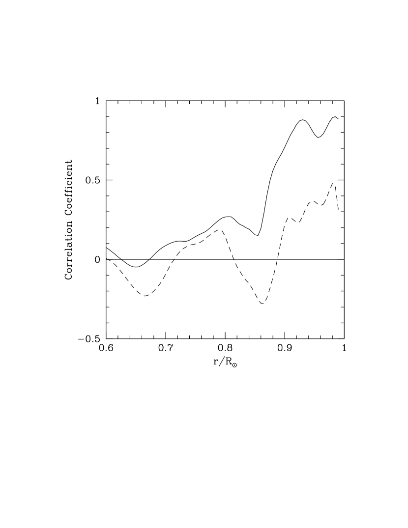
Figure 7: The correlation coefficient between the mean magnitude of the residuals in rotation rate in the latitude range 0–60^∘ and the average 10.7 cm radio flux during the period the data were obtained is plotted as a function of radius. The continuous line represents the result obtained when the residual is determined by subtracting the mean of only the smooth component of the rotation rate (obtained from coefficients $c_{1},c_{3},c_{5}$) from the total rotation rate. The dashed line is the result when the time-average of the full rotation rate is subtracted from the rotation rate at a given time.

At depths exceeding $0.1R_{\odot}$ the correlation between the zonal flow and the 10.7 cm flux becomes markedly weaker and there appears to be no correlation at a depth of $0.2R_{\odot}$. To show this result quantitatively, in Fig. 7 we plot the correlation coefficient between the average 10.7 cm flux over the period observations were made and the latitudinally averaged magnitude of $\delta\Omega$ as a function of radius. This figure shows that the correlation between the zonal flow and solar activity does not extend to the bottom of the convection zone. It probably also implies that the flow pattern itself does not penetrate through the convection zone. Similar conclusions can be drawn from Fig. 2, where the flow pattern is seen to change significantly below a radius of $0.9R_{\odot}$. The correlation coefficient shows a sudden drop around the radius of $0.89R_{\odot}$ and this could be considered to be the depth to which flow pattern penetrates. There is some difficulty in estimating the penetration-depth of the zonal flows to high precision because the errors in inversion increase with depth and it becomes increasingly difficult to detect any pattern by just looking at the results at different depths. But the sudden drop in the correlation coefficient around $0.89R_{\odot}$ is difficult to explain as being caused by an increase in the errors. Neither the errors, nor the resolution drops suddenly below $0.89R_{\odot}$ and hence we would expect a slower drop due to these factors. We can thus conclude that the zonal flow pattern penetrates to a depth of about $0.1R_{\odot}$.

As mentioned earlier, if instead of subtracting the mean rotation rate obtained from only the coefficients $c_{1},c_{3},c_{5}$, we subtract the mean of full rotation rate, the amplitude of residuals doesn’t show any increase with activity. This can also be seen in Fig. 7 which also shows the correlation coefficient for this case. This is due to the fact that the higher order coefficients $c_{7},c_{9},\ldots$ show an increase in amplitude with activity.

In order to study the radial behavior of the zonal flow, we have plotted the flow in Fig. 8 as a function of radius and time at a few selected latitudes. It can be seen that the pattern is quite different below about $r=0.9R_{\odot}$. This is just another indication that the flow pattern persists only in the outer layers of the Sun. At all latitudes there appears to be a tendency of the bands of faster or slower rotation to move up in radius with time. Though the significance of this upward movement is not clear as it is not seen at all times. Around the tachocline and below that there appear to be some pronounced oscillations with time at all latitudes. It is not clear if these are real or arise due to the regularization used in the inversion.

The oscillations in the region around the tachocline have also been studied by Howe et al. (2000b) who claim to see a 1.3 year periodicity in the equatorial rotation rate at a depth of $0.72R_{\odot}$. In order to verify this periodicity, in Figs. 9 and 10 we show the residuals in the rotation rate at a few selected depths and latitudes as a function of time. For clarity the error-bars are shown only for the 1.5d RLS inversions. The estimated errors in 2d inversions are comparable to those in 1.5d RLS at $r=0.95R_{\odot}$ and $0.90R_{\odot}$, while in deeper layers (Fig. 10) the error-bars on the results of the 2d inversions are about a factor of 2 lower than those of the 1.5d inversions. In order to make a proper comparison with Howe et al. (2000b) these residuals have been obtained by subtracting the time average of the full rotation rate from the rotation rate obtained from each data set. It is quite clear that there is a systematic variation with time in the rotation rate of the outer layers (which is clearly seen in Fig. 2 also though that was obtained by subtracting just the smooth part of the mean rotation rate). In deeper layers there are some variations which do not seem to be systematic. In order to test whether there are any periodic variations, we take a discrete Fourier transform of the data for the equator at $r=0.72R_{\odot}$. The resulting amplitude is shown in Fig. 11. There is no prominent peak in this spectrum at a period of 1.3 yr, or at any other period. Similar spectrum is obtained for other latitudes and depths in this region. Some of the apparent variations seen in the region around the tachocline can arise from the fact that in this region the rotation rate changes very rapidly with radius. Inversions tend to yield some average of the rotation rate in the neighborhood, and furthermore, since each data set has slightly different error estimates and mode set, the averaging would be different and one can expect to get some spurious variations.

4 Conclusions

Inversions to determine the solar rotation rate with data from GONG months 1–42, which mostly cover the rising phase of solar cycle 23, show a clear change in the rotation rate with solar activity. The zonal flow, which we have defined as residual in the rotation rate obtained by subtracting a time-average of a three-term fit to the rotation rate, shows bands of faster and slower rotation. These bands appear to move towards the equator with time. The magnitude of this time varying component is about 2 nHz. This pattern is similar to that found by Howe et al. (2000c) using helioseismic data from GONG and MDI projects. The amplitude of the flow pattern in our results is also similar to those in Howe et al. (2000c) as can be seen by comparing their Fig. 3 with our Fig. 9.

The mean magnitude of the pattern in the outer parts of the solar convection zone appears to increase with solar activity and is reasonably well correlated with the mean 10.7 cm flux which tracks solar activity. The correlation is seen up to a depth of about $0.1R_{\odot}$ (70 Mm). This appears to be depth to which the zonal flow pattern penetrates. Below this depth the temporal variations in the rotation rate do not appear to be significant. This inferred depth of zonal flow pattern is consistent with estimate of at least 60 Mm obtained by Howe et al. (2000c) using independent data sets and inversion techniques. Clearly, there is good agreement between different inversion results in the outer convection zone. There appears to be some hint that the flow pattern moves upwards with time, however, the statistical significance of this is as yet unclear.

We do not find any evidence of periodic changes in the solar rotation rate near the base of the solar convection zone. We find that the temporal variations at this depth are random in nature and probably represent statistical fluctuations. There is no clear periodic signal in the residual rotation rate with period less than 2 years at any depth. The present data length of 4 years does not allow us to study periodicities with longer time period. Some of this fluctuations may also arise from systematic errors in data.

Figure 1: The residuals in the rotation rate (zonal flow) shown as a function of latitude at a few selected depths and time. The continuous curves are for GONG months 1–3 centered around June 1995, short-dashed for June 1996, long-dashed for June 1997 and dot-dashed for June 1998. Error bars are shown only for the short-dashed curve for the sake of clarity. The error-bars are similar for all cases.

Figure 2: Contours of constant $\delta\Omega$ shown as a function of time and latitude at a few selected radius as marked above each panel. The continuous contours are for positive values and dotted for negative values. The contours are drawn at interval of 0.4 nHz.

Figure 3: A contour diagram of the residuals in the smooth component of the rotation rate. The results are shown as a function of time and latitude for a radius of $r=0.98R_{\odot}$. The continuous contours are for positive values and dotted for negative values. The contours are drawn at interval of 0.4 nHz.

Figure 4: A contour diagram of the residuals obtained by subtracting the time-average of the rotation rate from the rotation rate at a given time. The upper panel is the result obtained by 2d RLS inversion, while the lower panel is from 1.5d RLS inversion. The results are for radius $0.98R_{\odot}$. The contours have been drawn at intervals of 0.4 nHz, with continuous lines for positive contours and dotted lines for negative ones.

Figure 5: The difference in temporal averages of rotation rate obtained from the full profile and the smooth component ($\langle\Omega(r,\theta,t)\rangle-\langle\Omega_{s}(r,\theta,t)\rangle$) at two different depths are shown as a function of latitude. The continuous and dashed lines respectively, represent the difference at $r=0.98R_{\odot}$ and $0.90R_{\odot}$.

Figure 6: The mean magnitude of the residual in rotation rate (in the latitude range of 0–60^∘) at different depths plotted as a function of time and compared with an indicator of solar activity. The points joined by lines with error-bars show the zonal flow results for each of the available data sets. The squares show the average 10.7 cm flux during the corresponding period on a scale shown on the right side. Each panel corresponds to the radius marked inside the panel.

Figure 8: The residual in rotation rate plotted as a function of time and radius at a few selected latitudes as marked above each panel. The continuous contours are for positive values and dotted contours for negative values. The contours are drawn at intervals of 0.4 nHz

Figure 9: The residuals in the rotation rate shown as a function of time at a few selected depths and latitudes. These residuals were obtained by subtracting the time-average of the full rotation rate from the rotation rate obtained from each data set. The continuous lines with error-bars show the results obtained using 1.5d RLS inversion, while the squares mark the results from 2d RLS inversion. The latitude is marked in each panel, while the radius is marked just above the top panel.

Figure 10: The same as Fig. (9) but for different depths.

Figure 11: Results of a discrete Fourier transform of the rotation-rate residuals at the equator at $r=0.72R_{\odot}$. The continuous line shows the result using 1.5d RLS inversion while the squares mark the results from 2d RLS inversion. For clarity the error-bars are shown only for 1.5d results.

References

- (1) Antia, H. M., Basu, S., & Chitre, S. M. 1998, MNRAS, 298, 543
- (2) Basu S., 1997, MNRAS, 288, 572
- (3) Basu, S., & Antia, H. M. 2000a, Solar Phys., (in press)
- (4) Basu, S., & Antia, H. M. 2000b, Solar Phys., (in press)
- (5) Basu, S., Antia, H. M., & Tripathy, S. C. 1999, ApJ, 512, 458
- (6) Bhatnagar, A., Jain, K., & Tripathy, S. C. 1999, ApJ, 521, 885
- (7) Dziembowski, W. A., Goode, P. R., DiMauro, M. P., Kosovichev, A. G., & Schou, J. 1998, ApJ, 509, 456
- (8) Elsworth, Y., Howe, R., Isaak, G. R., McLeod, C. P., & New, R. 1990, Nature, 345, 322
- (9) Hill, F., Stark, P. B., Stebbins, R. T., et al. 1996, Science, 272, 1292
- (10) Howard, R., & LaBonte, B. J. 1980, ApJ, 239, L33
- (11) Howe, R., Komm, R., & Hill, F. 1999, ApJ, 524, 1084
- (12) Howe, R., Komm, R., & Hill, F. 2000a, Solar Phys., (in press)
- (13) Howe, R., Christensen-Dalsgaard, J., Hill, F., Komm, R. W., Larsen, R. M., Schou, J., Thompson, M. J., & Toomre, J., 2000b, Science (in press)
- (14) Howe, R., Christensen-Dalsgaard, J., Hill, F., Komm, R. W., Larsen, R. M., Schou, J., Thompson, M. J., & Toomre, J., 2000c, ApJL, (in press) (astro-ph/0003121)
- (15) Kosovichev A. G., 1996, ApJ, 469, L61
- (16) LaBonte, B. J., & Howard, R. 1982, Solar Phys., 75, 161
- (17) Libbrecht, K. G., & Woodard, M. F. 1990, Nature, 345, 779
- (18) Ritzwoller, M. H., & Lavely, E. M. 1991, ApJ, 369, 557
- (19) Schou, J. 1999, ApJ, 523, L181
- (20) Schou, J., Antia, H. M., Basu, S., et al. 1998, ApJ, 505, 390
- (21) Snodgrass, H. B. 1984, Solar Phys., 94, 13
- (22) Snodgrass, H. B. 1992, in The Solar Cycle, proc. NSO 12th Summer Workshop, ASPS 27, p205
- (23) Thompson M. J., Toomre J., Anderson E. R., et al. 1996, Science, 272, 1300
- (24) Toomre, J., Christensen-Dalsgaard, J., Howe, R., Larsen, R. M., Schou, J., & Thompson, M. J. 2000, Solar Phys., (in press)