On the supernovae heating of intergalactic medium

Abstract

We present estimates of the energy input from supernovae (SNe) into the intergalactic medium using (i) recent measurements of Si and Fe abundances in the intracluster medium (ICM) and (ii) self-consistent gasdynamical simulations that include processes of cooling, star formation, SNe feedback, and a multi-phase model of the interstellar medium. We estimate the energy input from observed abundances using two different assumptions: (i) spatial uniformity of metal abundances in the ICM and (ii) radial abundance gradients. We show that these two cases lead to energy input estimates which are different by an order of magnitude, highlighting a need for observational data on large-scale abundance gradients in clusters. Our analysis indicates that the SNe energy input can be important for heating of the entire ICM (providing energy of $\sim 1$ keV per particle) only if the ICM abundances are uniform and the efficiency of gas heating by SN explosions is close to $100\%$ ($\epsilon_{SN}\approx 1$, implying that all of the initial kinetic energy of the explosion goes into heating of the ICM).

The SNe energy input estimate made using simulations of galaxy formation is consistent with the above results derived from observed abundances, provided large-scale radial abundance gradients exist in clusters. For the cluster AWM7, in which such a gradient has been observed, the energy input estimated using observed metal abundances is $\sim 0.01$ and $\sim 0.1$ keV per particle for $\epsilon_{SN}=0.1$ and $\epsilon_{SN}=1$, respectively. These estimates fall far short of the required energy injection of $\sim 0.5-3$ keV per particle that appears to be needed to bring models of cluster formation into agreement with observations. Therefore, our results indicate that, unless the most favorable conditions are met, SNe alone are unlikely to provide sufficient energy input and need to be supplemented or even substituted by some other heating process(es).

1 Introduction

Hierarchical models of structure formation have been very successful in explaining many observed properties of galaxies and galaxy clusters. Nevertheless, some puzzling problems remain open. Several theoretical studies have demonstrated that some heating of gas, in addition to the heating during the gravitational collapse, is required to explain the observed properties of the intracluster medium (ICM). ? first showed that an early injection of energy results in correlations and evolution of bulk cluster properties (X-ray luminosity, gas temperature, etc.) that match observations. This conclusion was backed by numerical simulations: ? was able to get a better fit to the X-ray luminosity of the Coma cluster in his cosmological simulation by preheating the gas to $10^{7}$ K ($\approx 0.9$ keV), while ? showed that pre-heated clusters matched the observed slope of the correlation between X-ray luminosity and temperature. Recent semi-analytical studies of cluster evolution have reached similar conclusions (?; ?; ?; ?).

The exact amount of required energy injection depends on the epoch, and have been argued to be in the range of $0.5-3$ keV per gas particle (?; ?; ?; ?). Although the problem has been identified, it is not yet clear what processes can provide the required heating. It is clear that identification of these processes is crucial for a complete picture of cluster formation.

The candidate process which has been discussed most is supernovae-driven galactic winds. The gas of the galactic interstellar medium (ISM) can be heated by supernovae explosions and acquire energy comparable to or larger than its gravitational binding energy. This heated gas can then flow away and result in additional heating if the winds result in shocks when they encounter intergalactic gas. Although there is observational evidence for such winds in present-day galaxies (e.g., ?), theoretical models of winds are rather ill-constrained due to uncertainties in the efficiency of conversion of supernovae (SNe) explosion energy into thermal energy of the gas and other details.

Early estimates of possible energy input from SNe based on observed metal abundances showed that SNe are plausible candidates (e.g., ?; ?; ?). However, in these estimates it was assumed that the distribution of metals in the ICM is uniform and that the efficiency with which energy of SNe explosions can be converted into thermal energy of the gas is close to $100\%$. Therefore, there is a need for detailed estimates using new measurements of metal abundances in clusters and current galaxy formation models which have become much more advanced and sophisticated in the last several years.

Evaluations of SNe as a heating source have recently been performed by ? and ? using a semi-analytical approach to galaxy modelling. These authors conclude that it is unlikely that supernovae are the only source of heating. ? argue then that radiation from quasar population can provide the required heating much more easily.

In this paper we repeat previous estimates of the possible SNe energy input using updated values of observed ICM abundances and relaxing the assumption of abundance uniformity, motivated by recent observations (?; ?). We also make a separate estimate for the cluster AWM7, for which the radial abundance gradient was measured. The details of this estimate are presented in § 2. We complement this analysis with direct estimates of the energy input by counting the total number of supernovae exploded in all cluster galaxies throughout their evolution in self-consistent three-dimensional gasdynamical simulations of galaxy formation. The simulations include cooling, star formation, SNe feedback and a multi-phase model of the interstellar medium in galaxies and have been shown to match many fundamental observed correlations of galactic properties such as the galaxy luminosity function, the Tully-Fisher relation and its scatter, the color-magnitude sequence, and, perhaps most importantly, the evolution of the global star formation rate in the Universe. The details of the simulations are described in § 3. The energy input estimates are presented and compared in § 4 and discussed in § 5. We summarize our main results and conclusions in § 6.

2 Supernovae energy input from observed ICM metallicities

We will first estimate the energy input from SNe to the ICM using observed metallicities of the cluster gas. We have based the estimate on silicon (Si) and iron (Fe) abundances because these two elements have been most accurately measured for a large sample of galaxy clusters (?; ?). We use average ICM metallicities quoted in Table 1 and photospheric solar abundances of ? ($n_{Fe}/n_{H}=4.68\times 10^{-5}$ and $n_{Si}/n_{H}=3.55\times 10^{-5}$).

Given that the mass of an element $X_{i}$, $M_{X_{i}}$, within the cluster virial radius is known, the number of SNe type I and II required to produce this mass is equal to $f_{X_{i}}^{I}M_{X_{i}}/y_{I}(X_{i})$ and $(1-f_{X_{i}}^{I})M_{X_{i}}/y_{II}(X_{i})$, respectively. Here $f_{X_{i}}^{I}$ is mass the fraction of the element contributed by type I SNe, $y_{I}(X_{i})$ and $y_{II}(X_{i})$ are the mass-weighted yields of the element $X_{i}$ by SNe type I and II respectively. The SNe energy input can then be obtained by multiplying the number of SNe by the energy transferred to the gas during each SN explosion:

$$E_{SN}\approx M_{X_{i}}\left(f_{X_{i}}^{I}\frac{\epsilon_{SNI}E_{SNI}}{y_{I}(X_{i})}+(1-f_{X_{i}}^{I})\frac{\epsilon_{SNII}E_{SNII}}{y_{II}(X_{i})}\right),$$ (1)

where we denote $E_{SNI}$ and $E_{SNII}$ energies released in explosion of the two types of SNe, and $\epsilon_{SNI}$ and $\epsilon_{SNII}$ are fractions of the released energy left after the radiative losses during and after the explosion, which can be actually transferred in the form of thermal and kinetic energy to the ambient gas and lead subsequently to the increase of its entropy. There is a varying degree of uncertainty in our knowledge of the above parameters.

First of all, our estimate of the mass of an element depends on the assumption about uniformity of the observed metallicities. If strong radial abundance gradients exist in clusters, the observed metallicity is emission-weighted and therefore corresponds to the metallicity in the cluster core. Numerical simulations of cluster formation (?; ?) that include modelling of galaxy feedback predict the existence of strong radial metallicity gradients in the ICM, as well as patchy spatial distribution of metals. At present, however, it is not clear whether large-scale abundance gradients are universal in clusters. Although abundance gradients have been observed in several clusters (see, e.g., ?; ? and references therein), these are usually clusters that have a central cD galaxy and exhibit signatures of a central cooling flow (?). The spatial extent of the observed gradients coincides with that of the cooling flow region. It is thus unclear whether such central gradients imply the existence of a larger-scale gradient or they are simply due to the presence of a central cD galaxy and cooling flow.

Currently, abundances in the fainter, outer parts of clusters can be measured only for bright nearby systems. In a recent study, ?, found strong large-scale metallicity gradients in the nearby cluster AWM7. The observed iron abundance in this cluster decreases from $\approx 0.5\pm 0.05$ solar within the central $60h^{-1}{\ }{\rm kpc}$ to $\approx 0.2\pm 0.2$ at $300-500h^{-1}{\ }{\rm kpc}$. The radially averaged gradient can be well fitted by a $\beta$-model with a core radius equal to that of the gas and $\beta=0.8$. The Ezawa et al. measurement was the first in which the abundance gradient has been found far beyond the cluster core radius. It is not yet clear how common such large-scale gradients are. ? show that large-scale metallicity gradient are indeed observed in many clusters. It is clear, however, that strong large-scale gradients are not universal; for example, no strong gradient was detected in the Coma cluster (?). Clusters may therefore exhibit a variety of metal distributions and span a range in the ICM metallicities. In support of this, ?, present evidence that clusters without strong metallicity gradients have systematically lower metal abundances.

For our purposes it suffices to consider two possible extreme assumptions about the metal distribution. In reality the mass of metals will likely lie in between the masses computed under these assumptions. The first assumption is that the metallicity of the ICM is spatially uniform. Observationally, the metallicity derived from a spatially unresolved spectrum is emission-weighted. It is clear then that if a strong metallicity gradient is present in a cluster, the total mass of metals may be significantly overestimated under the assumption of spatial uniformity. Our second assumption is that the metallicity gradient of the form observed by Ezawa et al.: $Z(r)=Z_{0}[1+(r/r_{c})^{2}]^{-3\beta/2}$ is a universal property of the cluster ICM. We will assume $r_{c}=100h^{-1}{\rm kpc}$ and $\beta=0.8$ (?) for all clusters, normalizing $Z_{0}$ to a value such that $Z(r_{c})$ is equal to the observed value of metallicity. Most of the cluster emission comes from radii $<2r_{c}$, providing an approximate way to account for the emission-weighting of the metallicity. The core radius of $100h^{-1}{\ }{\rm kpc}$ is larger than the best fit value for the cluster AWM7 but is closer to a typical core radius of the gas distribution in rich clusters. In addition to the estimate for the whole range of cluster masses, we will present the SN energy input for the specific case of AWM7 for which the abundance gradient has been observed and its parameters measured.

Another source of uncertainty is the relative importance of type Ia SNe (parameter $f_{X_{i}}^{I}$) in the metal enrichment of the ICM (?; ?; ?). Therefore, in the case of iron, we will treat $f_{Fe}^{I}$ as a free parameter and calculate $E_{SN}$ for values ($f_{X_{i}}^{I}=0.0,0.5,1.0$). Silicon is a special case, because $y_{II}(Si)\approx y_{I}(Si)$. This renders $E_{SN}$ almost insensitive to a particular choice of $f_{Si}^{I}$. This insensitivity, together with the fact that silicon abundance was fairly accurately measured by ? and ?, effectively reduces the uncertainties and thus makes Si a very useful element for our estimate.

The third major source of uncertainty is the yields predicted by different theoretical models of SN explosions (?). The yields of SNe type II may depend on the initial metallicity of SNe, input physics of a model, and other factors. In our estimate we will use yields calculated by ? for metal-poor ($Z/Z_{\odot}=10^{-4}$) SNe with explosion energy of $\approx 1.2\times 10^{51}{\rm ergs}$ (model A) and metal-rich ($Z/Z_{\odot}=1$) SNe with explosion energy of $\approx 1.2\times 10^{51}{\rm ergs}$ for SN of mass $\leq 25{\rm M_{\odot}}$ and $\approx 2\times 10^{51}{\rm ergs}$ for SN of mass $>25{\rm M_{\odot}}$ (Model B). Model B has a higher explosion energy for very massive stars to reduce the effects of reimplosion of explosively synthesized ejecta, thus increasing the yields. The yields for these models approximately give the lower and upper limits of the current theoretical predictions (see ?; ?; ?). Given the wide spread in predictions of theoretical models, the supernovae energy input estimates from the observed metallicities have the uncertainty of up to $\sim 50\%$, in addition to other possible uncertainties.

We calculate the average yield of SNII by averaging the mass-dependent yields with a stellar initial mass function (IMF):

$$y_{II}(X_{i})=\frac{\int^{m_{u}}_{m_{l}}y_{II}(X_{i},m)\phi(m)dm}{\int^{m_{u}}_{m_{l}}\phi(m)dm}.$$ (2)

For the IMF we assume the (?) function, $\phi(m)\propto m^{-2.35}$, with the lower mass limit of $m_{l}=12M_{\odot}$ and $m_{l}=11M_{\odot}$ for the two yield models and the upper mass limit of $m_{u}=40M_{\odot}$. The SN with masses $<11M_{\odot}$ do not contribute significantly to the metal enrichment, while stars of mass $>40M_{\odot}$ are rare. Our choice of the Salpeter IMF does not affect the average yields significantly: averaging with considerably shallower ($\phi(m)\propto m^{-2}$) and steeper ($\phi(m)\propto m^{-2.7}$) IMFs results in average yields that differ by less than $10\%$ from the values for the Salpeter IMF. For SN type Ia, the yields appear to be independent of the SN mass. We use SNIa yields (see Table 1) predicted by the W7 model of ?, which is a model of simple deflagration. The yields for the supernovae of type Ia and type II used in our analysis are summarized in Table 1.

The energy released in a SN explosion ($E_{SNI}$ and $E_{SNII}$) also depends on a variety of factors (e.g. the mass of supernova). However, it can vary only by a factor of $\sim 2$ and we will therefore assume for simplicity that $E_{SNI}=E_{SNII}=1.2\times 10^{51}{\rm ergs}$ (e.g., ?). Not all of this initial kinetic energy of explosion is retained by the ejected gas. Analytical arguments (?; ?) and recent numerical simulations (?) suggest that at most $\sim 10\%$ of the initial kinetic energy of explosion can be ultimately transferred to the ambient gas. In particular, ? have numerically studied the evolution of the ejected material for a variety of densities and metallicities of the ambient gas and concluded that regardless of the ambient density and metallicity, ${{}_{>}\atop{{}^{\sim}}}90\%$ of the initial energy acquired by ejecta during the explosion is lost to radiation (see, however, discussion in § 5). Therefore, we will assume that only $10\%$ of the explosion can actually be transferred to the ambient gas: i.e., $\epsilon_{SNI}=\epsilon_{SNII}=0.1$. Here, we neglect the dependence of $\epsilon$ on environment, metallicity, and possible systematic differences between $\epsilon_{SNI}$ and $\epsilon_{SNII}$. However, according to ?, radiation losses are $\sim 90\%$ or more for most of the realistic environments and metallicities and the value of $\epsilon=0.1$ is a reasonable upper limit for both types of SNe. We note that the energy estimates from observed metallicities presented in Figs. 4–5 can be simply linearly scaled up or down for other values of $\epsilon$. Clearly, the energy of SNe explosions is actually released into the interstellar medium and needs then to be somehow transferred to the IGM. Even if such transfer is possible, it is likely that it would result in additional energy losses. The estimates we make should therefore be considered as the upper limits on the amount of the energy that could have been available for the IGM heating.

All of the estimates are made assuming the low-density flat cold dark matter model with cosmological constant ($\Lambda$CDM). The contributions of baryons, cold dark matter, and vacuum energy are: $\Omega_{b}=0.05$, $\Omega_{m}=0.25$, $\Omega_{\Lambda}=0.7$, respectively. We assume a Hubble constant of $H_{0}=70{\ }{\rm km{\ }s^{-1}{\ }Mpc^{-1}}$. The cluster virial radius and mass for this model are defined at the overdensity of $\approx 334$ and we assume the baryon fraction within the virial radius is $f_{b}=\Omega_{b}/\Omega_{m}\approx 0.17$.

Table 1: Parameters adopted in the estimate of energy input from observed metallicities

	Z	$y_{I}$	$y_{II}^{A}$	$y_{II}^{B}$
Si	0.65	0.158	0.124	0.158
Fe	0.32	0.744	0.096	0.153

3 Energy input from supernovae in numerical simulations of galaxy formation

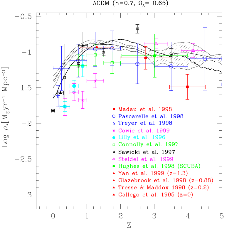
Figure 1: Comparison of star formation history in the Universe (points), estimated from the UV and H$\alpha$ luminosity densities, corrected for dust extinction, with the star formation history obtained in the gasdynamical simulations used in this paper. The solid lines indicate the average and scatter of the star formation history in eleven $5$ Mpc runs, while the thick solid line shows the star formation rate in $12$ Mpc run. All of the data points have been converted to the $\Lambda$CDM cosmology with $\Omega_{0}=1-\Omega_{\Lambda}=0.35$ and the Hubble constant of $H_{0}=70\rm{\ }km{\ }s^{-1}{\ }Mpc^{-1}$.

Figure 2: Correlation of the $z=0$ $B$-band absolute magnitude of simulated galaxies and number of SNe type II exploded in the galaxy throughout its history. The open circles represent simulated galaxies in $5$ Mpc runs, triangles represent galaxies in the $12$ Mpc run, and the solid line shows a linear fit to the correlation. Number of SNe, $N_{SN}$, is estimated as $N_{SN}=0.12M_{\ast}/22M_{\odot}$, where $M_{\ast}$ is the mass of gas converted into stars, $0.12$ is the fraction of the mass converted into stars with mass $>10M_{\odot}$, and $22M_{\odot}$ is the IMF-weighted mean supernova mass. Both numbers assume a Salpeter IMF.

The question we now ask is what energy, $E_{SN}^{g}$, can be expected to have been released in all the SNe in cluster galaxies throughout their evolution? This question can be answered only in the framework of a self-consistent model of galaxy formation. There are currently two independently developing approaches to modelling galaxy formation and evolution: semi-analytic models (SAMs; e.g., ?; ?; ? and references therein) and numerical models (e.g., ?; ?; ?). In this section we will make an estimate of $E_{SN}^{g}$ using numerical simulations of galaxy formation. The numerical techniques and physical ingredients of the model are described in ?. The model includes a self-consistent treatment of the dark matter and baryonic components and effects of cooling, star formation, and SNe feedback. Simulations include a multi-phase model of interstellar medium. Note that these simulations account only for SN type II so the contribution from SNI is therefore neglected in the estimate of $E_{SN}^{g}$.

The ideal simulation for our purpose would be a full modelling of cluster formation that would include formation of the cluster galaxies, their starformation and feedback. However, with the numerical code used here, this would require a significant sacrifice in the spatial dynamic range and mass resolution and would make it impossible to follow reliably the starformation and feedback processes. Such simulation awaits future higher dynamic range simulations using adaptive mesh refinement technique. We choose the following compromise. We use many small-box galaxy formation simulations to determine statistically the number of supernovae, $N_{\rm SN}$, that is expected to explode in a galaxy of a given absolute magnitude, $M_{\rm B}$. We then use this relation and assume a galaxy luminosity function in clusters to estimate how many supernovae could have exploded in a cluster of a given mass. The energy released in these SN explosions would provide an upper limit on the amount of energy available for IGM heating. While the number of SNe could be estimated by assuming a particular $N_{\rm SN}-M_{\rm B}$ relation, the use of simulations in this study spares us from making this additional assumption. As we describe below, the simulations reproduce many of the observed galactic properties which provides support to the used $N_{\rm SN}-M_{\rm B}$ relation.

The simulations of the COBE-normalized $\Lambda$CDM model ($\Omega_{0}=1-\Omega_{\Lambda}=0.35$; $\Omega_{b}=0.026$; $H_{0}=70{\rm{\ }km{\ }s^{-1}{\ }Mpc^{-1}}$, where $\Omega_{0}$, $\Omega_{b}$, and $H_{0}$ are present day values of the matter and baryon densities and the Hubble constant, respectively) used here are described in ?. A total of 11 simulations were run from different realizations of initial conditions. The size of the simulation boxes was fixed to $L_{box}=3.5h^{-1}{\ }{\rm Mpc}=5{\rm Mpc}$ and the simulations were run using $128^{3}$ grid cells and particles which gives mass and spatial resolution of $\approx 2\times 10^{6}h^{-1}{\ }{\rm M_{\odot}}$ and $\approx 27h^{-1}{\ }{\rm kpc}$, respectively. A total of $240$ galaxies, $140$ of which have $M_{B}(z=0)<-14$, were formed in all the runs combined. The observed color-magnitude diagram, luminosity function (LF), and Tully-Fisher relation of low-redshift galaxies are reproduced well by the simulated galaxies (?; ?). Simulations used here were done assuming SN feedback parameter of $A=200$ (see ?). This value of the parameter means a moderate efficiency of supernovae feedback and, correspondingly, relatively high star formation rate.

Figure 3: Correlation of the $z=0$ $B$-band absolute magnitude of simulated galaxies and number of SNe type II exploded in the galaxy prior to a given epoch $z$ ($z=0$: upper left panel; $z=0.5$ lower left panel; $z=1$: upper right panel; $z=2$: lower right panel. Symbol labeling is the same as in Fig. 2.

The redshift dependence of the global star formation rate averaged over all simulations is shown in Fig. 1 together with the current data on observed global star formation history in the Universe (see also ? for comparisons of other cosmological models). The observational data were collected from ?; ?; ?; ?; ?; ?; ?; ?; ?; ?; ?; ?, and ?. All data points correspond to measurements of comoving UV or $H\alpha$ luminosity densities. In order to transform to star formation densities, we have followed Madau’s prescription (?) to correct the original data for dust extinction and to transform the luminosity densities to star formation densities. All data points were properly rescaled to the $\Lambda$CDM cosmological model used in the numerical simulations. The figure shows that the simulation results are in agreement (within the errors) with the observed evolution of the global star formation rate. The star formation rate in the simulations may actually be a little higher than the average observed rate, implying hence a larger number of exploded SNe. As we derived the SN rate from the galactic star formation rate shown in Fig. 1, this figure may serve as an illustration of how the SN explosion rate evolves with time.

We have analyzed two additional simulations to assess the effects of resolution and box size. Particularly, the effects of resolution were checked by re-running one of the $5$ Mpc simulations with $256^{3}$ grid cells and particles (i.e., with eight times better mass resolution and twice the dynamic range). We have not found any significant changes in the global star formation rate or in the predicted number of supernovae (see below). To test the effects of the box size, we ran a simulation of $8.4h^{-1}{\ }{\rm Mpc}=12{\rm\ Mpc}$ box using $300^{3}$ grid cells and particles, which gives the same resolution as the $128^{3}$ $5$ Mpc runs but in a $2.4$ times larger box. The results of this simulations are shown in Figs. 1 and 2 together with the results of other runs. The figures show that results of the large-box simulation are in agreement with results of $5$ Mpc runs.

As we mentioned above, to estimate $E_{SN}^{g}$ expected from galaxies which end up in a cluster, we make use of the correlation between absolute magnitude of a galaxy at z=0 and number of type II SNe exploded in this galaxy throughout its evolution. The number of type II SNe exploded in a galaxy of absolute magnitude $M$, $N_{SN}(M)$, is computed as the fraction of gas mass converted into stars of mass $\geq 10M_{\odot}$ divided by the IMF-weighted mean SNe mass. We use the ? IMF, for which these numbers are $0.12$ and $22M_{\odot}$ (using lower and upper integration limits of $0.1M_{\odot}$ and $125M_{\odot}$), respectively.

Figure 2 shows $z=0$ correlation $N_{SN}(M_{B})$ for galaxies formed in the eleven $5$ Mpc and one $12$ Mpc $\Lambda$CDM runs. The correlation at $z=0$ can be well fitted by a linear fit (shown by solid line) of the form $\log(N_{SN})=a+bM_{B}$, with $a=1.411$ and $b=-0.344$. Figure 3 shows evolution of this correlation with redshift. The figure shows that by $z=2$ the number of exploded SNe is predicted to be $\approx 3-5$ smaller than the number exploded by $z=0$. Note that galaxies in our simulations are either isolated or are located in poor groups. It can be expected that formation of cluster galaxies occurs somewhat earlier than that of galaxies in poorer environments (by about $\Delta z\approx 1$, see, e.g., ?) and the results for $z>2$ should probably be interpreted as $z>3-3.5$ instead.

To estimate the supernovae energy input in a cluster of a given virial mass, $M_{vir}$, we convolve $N_{SN}(M_{B})$ fit with the ? galaxy luminosity function

$$\phi(M)=0.4\ln 10\phi_{\ast}x^{1+\alpha}e^{-x};{\ \ }x\equiv 10^{0.4(M_{\ast}-M)};$$ (3)

where normalization parameter $\phi_{\ast}$ is assumed to be equal to $\Delta_{vir}$ times its field value. The parameter $\Delta_{vir}$ is the expected virial overdensity in a given cosmological model and is $\approx 334$ for the $\Lambda$CDM model adopted for our estimate (e.g., ?; ?). The energy input is thus

$$E_{SN}^{g}(M_{vir})=E_{s}\Delta_{vir}\left(\frac{4\pi}{3}R_{vir}^{3}\right)\int\limits^{M_{b}}_{M_{f}}N_{SN}(M)\phi(M)dM;$$ (4)

where $E_{s}=\epsilon_{II}E_{SNII}$ is the energy input of a single supernova explosion, $\phi(M)$ is the field LF, $R_{vir}$ is the virial radius of the cluster, $M_{b}$ and $M_{f}$ are the bright and faint limits of integration, and $\epsilon_{II}$, $E_{SNII}$ have the same meaning as in the previous section.

The parameters of the luminosity function of galaxies in clusters appear to be similar to those of the field LF (?) and we will therefore neglect possible small differences between cluster and field LFs and cluster-to-cluster variations. We adopt parameters $M_{B}=-19.5$ and $\alpha=-1.2$ of the Schechter luminosity function consistent with recent measurements of $B$-band LF in the field (?; ?) and in clusters (?). The faint-end slope $\alpha$ is somewhat steeper than in LFs from most of other field surveys (e.g., ?; ?; ?). However, the steep value $\alpha=-1.2$ better matches the LF of cluster galaxies and the faint end slope of the LF of the simulated galaxies (see ?). Therefore, we adopt this value in our analysis along with the normalization of the field LF $\phi_{\ast}^{field}=0.02h^{3}{\rm Mpc^{-3}}$ (?). This value may be uncertain by a factor of two (see Table 1 in ?). The $E_{SN}^{g}$ estimate presented below is proportional to $\phi_{\ast}$ and can be simply rescaled for other values. We use the integration limits $M_{B}^{b}=-22$ and $M_{B}^{f}=-14$. The results are insensitive to adopting a brighter $M_{b}$ or a fainter $M_{f}$. For consistency, we use $\epsilon_{II}=0.1$ and $E_{SNII}=1.2\times 10^{51}{\rm ergs}$ adopted in the previous section.

4 Results

Figures 4 and 5 show results of the estimates described in the previous two sections. In Figure 4 we compare estimated energy input from SNe with the thermal energy of the ICM gas. Top row of Fig. 4 shows $E_{SN}$ estimate using observed ICM metallicities and model A for SNII yields, while the bottom row shows the same estimate for yield model B (see Table 1).

The thermal energy of the gas is computed as

$$E_{th}=6\pi\frac{k}{\mu m_{p}}\int\limits_{0}^{R_{vir}}\rho_{g}(r)T(r)r^{2}dr,$$ (5)

where $k$ is the Boltzmann constant, $m_{p}$ is the mass of proton, $\mu=0.6$ is the assumed mean molecular weight of the ICM plasma, $\rho_{g}(r)$ and $T(r)$ are its radial density and temperature profiles. A density profile $\rho_{g}(r)$ is assumed, and the temperature profile is calculated from the equation of hydrostatic equilibrium. In Fig. 4, we assume that gas is distributed similarly to dark matter, and is described by the ? (hereafter NFW), functional form,

$$\rho(r)=\frac{\rho_{s}}{(r/r_{s})(1+r/r_{s})^{2}}$$ (6)

with appropriate scaling of parameter $c=R_{vir}/r_{s}$ with cluster virial mass (NFW). The observed distribution of the ICM gas is more often described by the $\beta$-profile:

$$\rho(r)=\frac{\rho_{0}}{[1+(r/r_{c})^{2}]^{3\beta/2}},$$ (7)

where $r_{c}$ is the core radius, and the parameter $\beta$ controls the outer slope of the distribution. The thermal energy of gas distributed with the above density profile (for values of $r_{c}$ and $\beta$ consistent with the observed range) is only $\sim 10-20\%$ higher than $E_{th}$ of the NFW-distributed gas, the difference indistinguishable on the scale of Fig. 4.

Figure 4: Comparison of the energy input by SNe, $E_{SN}$, and thermal energy of the ICM gas, $E_{th}$, for clusters of different virial masses, $M_{vir}$. The four panels show estimates of $E_{SN}$ using observed metallicities of Si and Fe, as described in § 2; top row: using yield model A, bottom row: using yield model B (see Table 1). $E_{SN}$ are shown for the cases where the ICM metallicity is uniform throughout the cluster (dashed lines) and for the presence of a strong metallicity gradient (solid lines) (see § 2 for details). Solid triangles are estimates for the cluster AWM7, in which such gradient was observed. $E_{SN}$ was estimated for three different metal fractions contributed by type Ia SNe: $f_{X_{i}}^{I}=0.0,0.5,1.0$, corresponding to the shown groups of three curves and points (the top curves/points correspond to $f_{X_{i}}^{I}=0.0$ and the bottom to $f_{X_{i}}^{I}=1.0$). $E_{th}(M_{vir})$ (dotted line; the same in all panels) was calculated assuming the gas is distributed similarly to the dark matter (NFW distribution). $E_{th}$ of the gas distributed with the “$\beta$-model” is larger by $\sim 10-20\%$. The energy released by type II SNe in the numerical simulations is shown by dot-dashed lines (the same in all panels).

Figure 5: Energy per gas particle injected by SNe ($=E_{SN}/N_{p}$, where $N_{p}=f_{b}M_{vir}/(\mu m_{p})$). The curves and points have the same meaning as in Fig. 4. The upper row shows the estimate of $E_{SN}$ from the observed metallicity assuming model A for SNII yields, while the bottom row shows the same estimate assuming model B.

Figure 4 shows that expected energy input from SNe is, depending on the assumed uniformity of the ICM metallicity, $\sim 5-10\%$ of the gas thermal energy for poor clusters ($M_{vir}\sim 10^{14}h^{-1}M_{\odot}$) and ${{}_{<}\atop{{}^{\sim}}}5\%$ for rich clusters ($M_{vir}\sim 10^{15}h^{-1}M_{\odot}$). In case of the strong metallicity gradients these numbers are $\approx 3\%$ and ${{}_{<}\atop{{}^{\sim}}}1\%$, respectively. The estimates from both Si and Fe agree very well between each other, for $f_{Fe}^{I}{{}_{<}\atop{{}^{\sim}}}0.5$. Supernova energy input estimated from the numerical simulations agrees well with $E_{SN}$ derived from observed metallicities in the case where a strong metallicity gradient is allowed. This implies that if metallicity gradients exist in clusters, simple galaxy formation models with the Salpeter IMF will have no difficulty in accounting for the observed amount of metals in clusters.

Figure 4 also shows estimates for the cluster AWM7 for which a large-scale abundance gradient has been observed and its parameters measured (?). The estimate was made using the observed metallicity gradient: $Z(r)=Z_{0}[1+(r/r_{c})^{2}]^{-3\beta_{Z}/2}$ with $Z_{0}=0.59$ and $\beta_{Z}=0.8$, where the core radius $r_{c}=57.5h^{-1}{\ }{\rm kpc}$ is equal to that of the gas distribution. The gas distribution is described by the similar $\beta$-profile with $\beta_{g}=0.58$ (see ? for details). We have made estimates for different gas fractions, $f_{b}$, within the cluster virial radius but the results are only mildly sensitive to a particular value of $f_{b}$; the estimates shown in figs. 4 and 5 were made assuming $f_{b}=0.2$. The energy input estimate for AWM7 lies even lower than the solid lines at this mass because to calculate the latter we have assumed a core radius of $r_{c}=100h^{-1}{\ }{\rm kpc}$, which results in a higher mass of metals and consequently larger estimated $E_{SN}$.

Table 2: Estimates of numbers of SNe and masses in Fe and Si for clusters of different masses (all masses are in $h^{-1}{\ }{\rm M_{\odot}}$).

Cluster mass	$10^{14}$	$5\times 10^{14}$	$10^{15}$
$N_{\rm SN}$ (simulations)	$7.8\times 10^{9}$	$3.9\times 10^{10}$	$7.8\times 10^{10}$
$N_{\rm SN}$ (for 1 keV per particle)	$4.9\times 10^{11}$	$2.5\times 10^{12}$	$4.9\times 10^{12}$
$M_{\rm Fe}$ (observed, assuming $Z$-gradient)	$2.7\times 10^{9}$	$8.8\times 10^{9}$	$1.5\times 10^{10}$
$M_{\rm Fe}$ (observed, uniform distribution)	$1.4\times 10^{10}$	$7.0\times 10^{10}$	$1.4\times 10^{11}$
$M_{\rm Si}$ (observed, assuming $Z$-gradient)	$2.1\times 10^{9}$	$6.9\times 10^{9}$	$1.2\times 10^{10}$
$M_{\rm Si}$ (observed, uniform distribution)	$1.1\times 10^{10}$	$5.5\times 10^{10}$	$1.1\times 10^{11}$

For reference, table 2 gives predictions for the numbers of type II SNe in clusters of different masses based on our model (line 1), as well as the total masses of Fe and Si inferred from observations with assumptions of metallicity gradient and uniform metal distribution (lines 3-6). The table also gives the number of SNe required to deposit 1 keV per gas particle into the ICM (line 2), estimated assuming that average supernova deposits $1.2\times 10^{50}$ ergs. The mass of metals predicted in our model can be easily obtained by multiplying the number of SNe in line 1 of table 2 by the corresponding mass-weighted yield given in Table 1. Note, however, that the predicted number refers to the type II SNe only, and the predicted mass of metals is thus only due to SNIIe.

The question we would ultimately like to address is whether the energy input from SNe can noticeably affect the thermal state of the ICM. To answer this question, we need to know what energy input is needed to account for the observed properties of the ICM. It is not completely clear what energy is required. However, on theoretical grounds (?; ?) it is known that model predictions are in better agreement with the data when gas is assumed to be preheated (by some non-gravitational process) at an early moment. The preheating results in gas evolution corresponding to a higher adiabat, which affects the evolution of the accreted gas (in particular, some of the accreted gas may avoid being strongly shocked).

Numerical simulations (?; ?; ?; ?) and semi-analytic models of cluster evolution (?; ?; ?; ?; ?) confirm that preheating results in cluster properties that are more in accord with observations. For example, to simulate SNe heating ? preheats the gas in his gasdynamic simulations by injecting 1 keV of energy per nucleon of gas, or, for plasma with primordial composition, $\approx 0.5{\rm keV}$ per gas particle. ? assume in their model that SNe preheat the intergalactic gas to temperatures of $\approx 0.5-0.7$ keV, which corresponds to $(3/2)kT\approx 0.75-1.0{\rm keV}$ per gas particle. ? and ? argue based on their semi-analytic calculations that the energy injection of $\sim 2-3$ keV per particle is required to bring model predictions in accord with observations.

We can compare our estimate of $E_{SN}$ to these numbers calculating the energy per gas particle as $E_{SN}/N_{p}$, where $N_{p}=f_{b}M_{vir}/(\mu m_{p})$ is the number of gas particles within the virial radius of cluster. Figure 5 shows $E_{SN}/N_{p}$ for $E_{SN}$ estimated from Si and Fe and from galaxy formation simulations. The figure shows that the maximum energy per particle of $\approx 0.1{\rm keV}$ can be injected by SNe if the ICM metallicity is homogeneous, while in the case of a strong metallicity gradient the typical energy per gas particle is only a few tens eV. In particular, the estimate of $E_{SN}$ for the cluster AWM7 is only $\sim 0.002-0.01$ keV per particle. The corresponding estimate from galaxy formation simulations is $\sim 10^{-2}{\rm keV}$ per particle. These numbers are $\sim 5-20$ times smaller than the typical energy injection assumed in the cluster formation models quoted above.

5 Discussion

The results presented in § 4 allow us to assess the conditions required for the SNe energy input to be important in galaxy clusters. The primary conditions that are implied by our estimate of $E_{SN}$ from the observed abundances of Si and Fe are (i) large-scale uniformity of the metal abundances throughout the cluster volume and (ii) near $100\%$ efficiency in transfer of the energy of SN explosion to the thermal energy of the IGM gas. The latter assumption is rather unlikely and the energies derived from the observed abundances should therefore be considered as the upper limits on the amount of SN energy that could have heated the IGM.

There are but a few theoretical predictions and observational data concerning the degree of uniformity of the metal distribution in clusters. Based on the numerical simulations that include galaxy feedback and metal enrichment, ? and ? predict that large-scale metallicity gradients should exist in clusters. On the observational side, ? observed such a gradient in cluster AWM7. More recently, ? reported similar large-scale ($R{{}_{<}\atop{{}^{\sim}}}0.5-1{\ \rm Mpc}$) metallicity gradients detected using ASCA observations for several other clusters. It is not clear, however, whether such gradients are ubiquitous. Our estimates of energy input from observed metal abundances differ by a factor of $\sim 5-10$ if we assume a uniform distribution of metals versus metallicity gradients of the type observed in AWM7. New, deep observations of ICM metallicity profiles are therefore crucial to make this estimate much more reliable. With the launch of the Chandra X-ray satellite, such observations should become available. Our estimate of the SN energy input for AWM7 is two orders of magnitude lower than energy input which seem to be required to sufficiently preheat the ICM gas.

Incidentally, the existence of large-scale abundance gradients in clusters would solve the problem of the total iron mass in clusters. ? and ? show that if the contribution of type I SNe to the iron production in clusters is relatively small, the total iron mass in the ICM is too large to be explained by type II SNe produced with Salpeter IMF. ? argue, however, that this solution is unattractive because it makes it difficult to explain the metallicities and radial abundance gradients in massive elliptical galaxies. It is clear from our analysis that the existence of large-scale abundance gradients in the ICM can reduce the estimate of the iron mass by up to an order of magnitude, thereby eliminating the need for a large number of SNII and flatter IMF.

The predictions of the SNe energy input, $E_{SN}^{g}$, of the numerical simulations of galaxy formation presented in this paper, although consistent with observed evolution of the global starfomation rate in the Universe, are somewhat lower than the estimate from the metal abundances, $E_{SN}^{m}$. The estimates $E_{SN}^{g}$ and $E_{SN}^{m}$ agree reasonably well if a metallicity gradient is assumed and the contribution of type Ia SNe to the iron enrichment is $>50\%$. In particular, the $E_{SN}^{g}$ estimate is actually higher than estimate of $E_{SN}^{m}$ for AWM7. However, the energy input in this case is of the order of $10-50$ eV per gas particle, which is far short of the energy injection typically assumed to bring theoretical models in accord with observations: $\sim 0.5-2$ keV per particle. The estimate will still be short by a factor of $\sim 5-10$ even if $100\%$ of the energy of every SN explosion goes into heating the ICM gas.

The above conclusions are for clusters of virial mass $M_{vir}{{}_{>}\atop{{}^{\sim}}}10^{14}h^{-1}{\ }{\rm M_{\odot}}$. Figure 4 shows that the ratio of predicted SNe energy input to the thermal energy of the ICM gas increases by about an order of magnitude as the mass is decreased from $10^{15}h^{-1}{\ }{\rm M_{\odot}}$ to $10^{14}h^{-1}{\ }{\rm M_{\odot}}$. This trend means that the SNe energy input may be much more important for clusters of mass $M_{vir}{{}_{<}\atop{{}^{\sim}}}5\times 10^{13}h^{-1}{\ }{\rm M_{\odot}}$ than for more massive clusters. The mass $5\times 10^{13}h^{-1}{\ }{\rm M_{\odot}}$ corresponds to the ICM temperature of $\approx 2$ keV (e.g., ?), while deviations from non-similarity are observed in real clusters for temperatures of ${{}_{<}\atop{{}^{\sim}}}2$ keV (?; ?). Nevertheless, it appears that quantitatively our conclusions will stand for poor clusters. The entropy of the preheated gas required to explain observations is $\sim 100{\ }{\rm keV{\ }cm^{2}}$ (?) which corresponds to an energy of $\approx 1.5(n_{e}/10^{-3}cm^{-3})^{2/3}$ keV per particle, where $n_{e}$ is electron number density. Thus, the energy injection into the gas in cluster cores ($n_{e}\sim 10^{-3}{\rm\ cm^{-3}}$) is about $1.5$ keV per particle. Semi-analytical calculations of ? and ? show that the energy injection required to explain the data may be even higher: $\sim 2-3$ keV per particle.

Such energy input is marginally consistent with our $E_{SN}^{m}$ estimate in the case of uniform metallicities and $\epsilon\approx 1$. For the case of metallicity gradients, $E_{SN}^{m}$ is more than an order of magnitude lower. The energy input, $E_{SN}^{g}$, predicted from numerical simulations is even lower and is $\approx 0.1$ keV per particle even for $\epsilon=1$. Therefore, the conclusion we draw from this analysis is that it is unlikely that the energy input from SNe is sufficient to preheat the intracluster gas to the required entropy, unless all of the explosion energy goes into heating of the gas and metal abundances are uniform throughout the ICM. Moreover, in light of the $E_{SN}^{g}$ estimates, the SN energy input can only be important if starformation rate in cluster environments is a factor of 10 higher than the average cosmic rate. Similar conclusions were reached by ?, ?, and ?. Recently, ? have also used observed abundance of Si in the ICM to estimate possible SNe heating and found that the implied SNe energies would not be sufficient to heat the entire cluster gas to the required levels (note that this estimate was done assuming uniform distribution of Si and $\epsilon_{SN}=1$). He pointed out, however, that SNe could still be the source of heating if only the gas in cluster cores was heated. In this case, heating would have to occur after or during formation of a cluster, not at early epochs as was assumed previously, but sufficiently early enough to be consistent with lack of evolution of metal abundances at lower redshifts ($z{{}_{<}\atop{{}^{\sim}}}1$; ?). Details and quantitative predictions of such a scenario are yet to be worked out.

It is obvious that there are a number of uncertainties in our estimates of the SNe energy input. The estimates of $E_{SN}^{m}$ made with the assumption of uniform ICM metallicity are by a factor $\sim 3-10$ higher than the corresponding estimates in the case when a strong metallicity gradient is assumed. This uncertainty not only makes the $E_{SN}^{m}$ estimate uncertain, but also hinders comparisons of metal abundances predicted by galaxy formation models with observations. This will likely be resolved in the near future with the advent of new, deep X-ray observations of clusters, but it is a major limitation at present. Currently, only one robust measurement of large-scale metallicity gradient has been obtained (?). This cluster, AWM7, confirms the existence of strong metallicity gradients and the estimate of $E_{SN}^{m}$ for this particular cluster supports our conclusions. It is not clear, however, how universal such gradients are in clusters.

Note also that our estimates are based on average abundances of Si and Fe from a large sample of clusters. Abundances in individual clusters may vary by a factor of ${{}_{>}\atop{{}^{\sim}}}2-3$. Thus, for example, abundances of Si and Fe (in solar units) vary in the range $\sim 0.1-1$ and $\sim 0.15-0.45$, respectively (?; ?). The energy estimates for individual clusters may therefore also vary by a corresponding factor.

The theoretical yields of Si and Fe from type Ia and type II SNe used in our analysis depend on specifics of the explosion model. The Si yields from SNIa may be uncertain by a factor of two (?; ?), while all models predict similar (to $\sim 10\%$) yields of iron. The yields of SNII for Si and Fe vary by $\sim 30-40\%$ between different models (e.g., ?). Yield models A and B used in our analysis approximately represent the range of predictions and should therefore provide a fair estimate of uncertainty. Our conclusions hold for both yield models.

The fraction of supernova explosion energy that can be available for gas heating is also rather uncertain. ? and ? give analytical arguments that this fraction should be $\sim 0.1$. These arguments are supported by recent direct numerical simulations of ? who studied radiative losses of a SN remnant (SNR) for a grid of densities and metallicities of the ambient gas. The arguments and simulations, however, assume spherically symmetric evolution of SNRs in ambient gas of uniform density. The efficiency may be higher if the topology of ambient gas density is very assymetric and the gas has been swept up and preheated by previous, recently exploded SNe (?). This, for example, may be the case during a strong starburst (e.g., ?). The parameter $\epsilon$ is thus likely to be environment dependent and the average value would be determined by the relative number of SNe exploding during periods of quiescent star formation vs. the number of SNe exploding in starbursts. Regardless of the actual value, considerable radiation losses are expected and therefore it seems very unlikely that the efficiency is close to $100\%$ ($\epsilon=1$).

Beside the problem of heating efficiency, it is also not clear how the heated interstellar gas and released SN energy is transferred to the IGM (or ICM). Several transfer mechanisms have been suggested. Gas may be blown away from galaxies by supernova-driven winds (?; ?; ?) which subsequently shock the IGM gas. Evidence for winds is indeed observed in some starburst galaxies (e.g., ?). However, only a small fraction of gas is expected to be blown away by starbursts in massive galaxies (e.g., ?, ?) and therefore ejected gas can only constitute a small fraction of ICM. Clearly, the same questions arise when we consider how energy released by SNe can actually heat the IGM. If only a fraction of this energy is delivered to IGM, this effectively means a smaller value of $\epsilon_{SN}$ and strengthens our conclusions.

The gas can also be transferred to the ICM by ram pressure (e.g., ?) and tidal stripping. The efficiency of ram pressure in clusters is not well known. Recent numerical simulations, however, suggest that it may actually be rather low (?). The tidal stripping is probably the most efficient mechanism of delivering ISM gas to the intracluster medium, especially for low surface brightness galaxies (?). However, in this case the gas is transferred to the ICM relatively late, after the epoch of cluster formation, when a sufficiently deep potential well is formed. This is in conflict with high metal abundances observed in high-redshift clusters (?; ?).

Recently, ? suggested that metal-enriched gas can be ejected at early epochs during galactic mergers. This mechanism may transfer metal-rich hot interstellar gas into IGM, where it can be further heated by shocks developed during a merger or after an encounter between ejected material and the ambient IGM gas. Despite the abundance of possible processes, it is not clear which process (or combination thereof) is responsible for the transfer of gas from galaxies into the intergalactic medium. It is clear, however, that this question needs to be clarified if SNe are to be considered a viable source of IGM heating.

We have made a number of assumptions to estimate $E_{SN}^{g}$ from the galaxy formation simulations. Changing some of these assumptions can change the energy input estimate. First of all, our assumption of Salpeter IMF directly affects the number of SNe per given mass of formed stars. IMFs Flatter than a Salpeter result in a larger number of supernovae and thus in a larger energy input for the same star formation rate. For instance, a 10% flatter slope with respect to Salpeter’s results in a 50% increase in the number of SNe, given the same low-mass limit of the IMF. Indeed, a flatter IMF has been suggested as an explanation for the observed iron abundances in clusters (e.g., ?; ?). However, note that ? argue that flatter IMF is not consistent with the evolution of elliptical galaxies. The number of SNe depends also on the low-mass limit of the IMF, although in a less sensitive manner. Thus, an increase of the lower-mass limit by a factor of 2 (from 0.1 to 0.2 $M_{\odot}$) results in an increase factor of 1.3 in the number of SNe.

To calculate the number of SNe exploded during a Hubble time in all cluster galaxies we have assumed that the number density of galaxies in clusters is equal $(1+\Delta_{vir})$ times its field value. This means that clusters represent the same fluctuation in number of galaxies as in their total mass. Although this is a reasonable assumption, we note that in the $\Lambda$CDM model (as well as in other low-matter density CDM cosmologies) studied here, a certain amount of anti-bias ($b\sim 0.5$) is required for the model to be consistent with observed galaxy clustering (?; ?; ?). This anti-bias arises primarily in the densest regions of galaxy groups and clusters (?). For an anti-bias of $b\approx 0.5$ the number density of galaxies would be two times lower than assumed in our analysis, which would reduce the estimated energy input by a factor of two.

We neglected possible differences between the shape of the field and cluster luminosity functions. These differences appear to be rather small for the $B$-magnitude LF used here (?), and we therefore think that the uncertainty associated with this assumption is relatively small.

A more important assumption is that the global star formation histories of field and cluster galaxies are similar. At present, there is no convincing evidence otherwise. ?, for example, argue that star formation activity in cluster galaxies is not very different from that in the field. They argue, in fact, that field galaxies may produce more stars (and more type II SNe) than cluster galaxies in which the star formation is being gradually turned off after their infall onto cluster. This is in fact consistent with theoretical predictions of ? who present models for the evolution of the SN rate in clusters and the field. They predict that the rate in clusters is higher than in the field only at $z{{}_{>}\atop{{}^{\sim}}}3.5$, while at lower redshifts it is actually lower due to a decreased contribution from SNe in spiral galaxies. Their predictions for the overall starformation rate in clusters are almost an order of magnitude lower than the starformation rate in the simulations presented here at $z{{}_{<}\atop{{}^{\sim}}}3.5$ and are higher at higher redshifts. It seems unlikely, however, that their prediction can account for the required tenfold increase in number of SNe because only a small fraction of SNe in cluster galaxies explode at ${{}_{>}\atop{{}^{\sim}}}4$. We therefore conclude that possible differences in starformation histories between cluster and field galaxies are too small to change our conclusions.

Nevertheless, it is known that rich clusters have properties different than if they would have simply had been constructed from massive ellipticals and small galaxy groups (?; ?; ?). Ellipticals and galaxy groups appear to have smaller gas fractions and lower metal abundances than rich clusters do. In particular, the ratio of iron mass in the ICM to the total blue luminosity of cluster galaxies is consistently higher for clusters than for groups (?). It appears also that parameters of the models of elliptical galaxies that are tuned to produce the observed metal abundances in the ICM are inconsistent with abundance measurements in individual ellipticals, the problem which cannot be solved by adjusting the SNIa contribution to the metal enrichment (?). These problems may indicate that an important component is missing in our understanding of the ICM enrichment history and cluster evolution. However, our conclusions about the importance of SNe energy input can only change if the star formation rate in the volume from which the cluster forms is significantly higher at all epochs than that star formation rate in the field.

6 Conclusions

We have presented estimates of the possible energy input by supernovae into the intracluster medium. Although these estimates are prone to a number of uncertainties, we have defined conditions which determine whether SNe can be a significant source of ICM heating. The following main conclusions can be drawn from our analysis.

The SNe energy input, $E_{SN}^{m}$, estimated from observed ICM abundances of Si and Fe is only significant ($\sim 1$ keV per particle) when we assumed that the distribution of metals in the ICM is uniform (no significant radial gradients) and that $\sim 100$% of individual SN explosion energy goes into heating the ambient gas followed by negligible cooling ($\epsilon\approx 1$) (see § 2). If large-scale metallicity gradients are assumed in clusters, the estimated energy input is $\sim 0.1-0.5$ keV per particle for $\epsilon=1$ and, correspondingly, $0.01-0.08$ keV per particle for a more realistic value of $\epsilon=0.1$.

As an example, we present estimates of the energy input for the cluster AWM7 for which the abundance gradient has been measured. We find that the observed abundance of iron in this cluster implies a SNe energy input of ${{}_{<}\atop{{}^{\sim}}}0.01$ and ${{}_{<}\atop{{}^{\sim}}}0.1$ keV per particle for $\epsilon=0.1$ and $\epsilon=1$, respectively.

The energy input, $E_{SN}^{g}$, estimated using self-consistent three-dimensional numerical simulations of galaxy formation which include effects of shock heating, cooling, SN feedback, and multi-phase model of ISM, are $\approx 0.01$ and $\approx 0.1$ keV per gas particle for values of efficiency parameter $\epsilon=0.1$ and $\epsilon=1$, respectively. These values are somewhat lower than the values of $E_{SN}^{m}$ (but are in good agreement with estimates for the AWM7). Nevertheless, the two estimates agree reasonably well if the existence of large-scale abundance gradients is assumed in clusters. We therefore emphasize the importance of new measurements of large-scale metallicity gradients for testing the theoretical models.

Our estimates of the SN energy input in all cases, except the case of uniform ICM abundances and $\epsilon=1$, fall short of the energy injection of $\sim 0.5-3$ keV per particle required to bring theoretical models of cluster formation in accord with observations. This suggests that supernovae are unlikely to be the only source of the IGM heating and should possibly be supplemented (or substituted) by some other heating mechanism. Similar conclusions have been reached in recent studies of ?, ?, and ?. ? propose radiation from quasars as an alternative heating mechanism. This opens discussion of new possible processes for what appears to be a required high-redshift preheating of the intergalactic medium.

References

- Abadi et al. (1999) Abadi, M., Moore, B., & Bower, R. 1999, Mon. Not. Roy. Astron. Soc., in press, astro-ph/9903436.
- Allen & Fabian (1998) Allen, W. & Fabian, A. 1998, Mon. Not. Roy. Astron. Soc. 297, L63–L68.
- Anders & Grevesse (1989) Anders, E. & Grevesse, N. 1989, Geochimica et Cosmochimica Acta 53, 197–214.
- Babul & Rees (1992) Babul, A. & Rees, M. J. 1992, MNRAS 255, 346–350.
- Bahcall et al. (1995) Bahcall, N. A., Lubin, L. M., & Dorman, V. 1995, ApJL 447, L81–L85.
- Balogh et al. (1999a) Balogh, M., Babul, A., & Patton, D. 1999, Mon. Not. Roy. Astron. Soc., in press, astro-ph/9809159.
- Balogh et al. (1999b) Balogh, M., Morris, S., Yee, H., Carlberg, R., & Ellingson, E. 1999, Ap. J., in press, astro-ph/9906470.
- Baugh et al. (1996) Baugh, C. M., Cole, S., & Frenk, C. S. 1996, Mon. Not. Roy. Astron. Soc.283, 1361–1378.
- Brighenti & Mathews (1999) Brighenti, F. & Mathews, W. G. 1999, ApJ 515, 542–557.
- Cavaliere et al. (1997) Cavaliere, A., Menci, N., & Tozzi, P. 1997, ApJL 484, L21–L24.
- Connolly et al. (1997) Connolly, A. J., Szalay, A. S., Dickinson, M., Subbarao, M. U., & Brunner, R. J. 1997, Ap. J. Lett. 486, L11–+.
- Cowie et al. (1999) Cowie, L., Songaila, A., & Barger, A. 1999, A. J., in press, astro-ph/9904345.
- Da Costa et al. (1994) Da Costa, L. N., Geller, M. J., Pellegrini, P. S., Latham, D. W., Fairall, A. P., Marzke, R. O., Willmer, C. N. A., Huchra, J. P., Calderon, J. H., Ramella, M., & Kurtz, M. J. 1994, Ap. J.424, L1–L4.
- David et al. (1991) David, L. P., Forman, W., & Jones, C. 1991, ApJ 380, 39–48.
- David (1997) David, L. P. 1997, ApJL 484, L11–L15.
- Dupke & White (1999) Dupke, R. & White, R. 1999, Ap. J., submitted, astro-ph/9902112.
- Eke et al. (1996) Eke, V. R., Cole, S., & Frenk, C. S. 1996, MNRAS 282, 263–280.
- Elizondo et al. (1999a) Elizondo, D., Yepes, G., Kates, R., & Klypin, A. 1999, New Astronomy 4, 101–132.
- Elizondo et al. (1999b) Elizondo, D., Yepes, G., Kates, R., Müller, V., & Klypin, A. 1999, Ap. J.515, 525–541.
- Evrard & Henry (1991) Evrard, A. E. & Henry, J. P. 1991, ApJ 383, 95–103.
- Evrard (1990) Evrard, A. E. 1990, ApJ 363, 349–366.
- Ezawa et al. (1997) Ezawa, H., Fukazawa, Y., Makishima, K., Ohashi, T., Takahara, F., Xu, H., & Yamasaki, N. Y. 1997, Ap. J. Lett. 490, L33–+.
- Finoguenov et al. (2000) Finoguenov, A., David, L., & Ponman, T. 2000, Ap. J., submitted, astro-ph/9908150.
- Fukazawa et al. (1998) Fukazawa, Y., Makishima, K., Tamura, T., Ezawa, H., Xu, H., Ikebe, Y., Kikuchi, K. I., & Ohashi, T. 1998, Publications of the Astronomical Society of Japan 50, 187–193.
- Gallego et al. (1995) Gallego, J., Zamorano, J., Aragon-Salamanca, A., & Rego, M. 1995, Ap. J. Lett. 455, L1–+.
- Gibson et al. (1997) Gibson, B. K., Loewenstein, M., & Mushotzky, R. F. 1997, Mon. Not. Roy. Astron. Soc. 290, 623–628.
- Glazebrook et al. (1999) Glazebrook, K., Blake, C., Economou, F., Lilly, S., & Colless, M. 1999, Mon. Not. Roy. Astron. Soc., in press, astro-ph/9808276.
- Gnedin & Ostriker (1997) Gnedin, N. Y. & Ostriker, J. P. 1997, ApJ 486, 581–598.
- Gottlöber et al. (2000) Gottlöber, S., Klypin, A. A., & Kravtsov, A. V. 2000, Ap. J., submitted, astro-ph/0004132.
- Gunn & Gott (1972) Gunn, J. E. & Gott, I. 1972, ApJ 176, 1–19.
- Hattori et al. (1997) Hattori, M., Ikebe, Y., Asaoka, I., Takeshima, T., Boehringer, H., Mihara, T., Neumann, D. M., Schindler, S., Tsuru, T., & Tamura, T. 1997, NAT 388, 146–148.
- Heckman et al. (1990) Heckman, T. M., Armus, L., & Miley, G. K. 1990, ApJS 74, 833–868.
- Hughes et al. (1993) Hughes, J. P., Butcher, J. A., Stewart, G. C., & Tanaka, Y. 1993, Ap. J. 404, 611–619.
- Hughes et al. (1998) Hughes, D. H., Serjeant, S., Dunlop, J., Rowan-Robinson, M., Blain, A., Mann, R. G., Ivison, R., Peacock, J., Efstathiou, A., Gear, W., Oliver, S., Lawrence, A., Longair, M., Goldschmidt, P., & Jenness, T. 1998, Nature 394, 241–247.
- Jenkins et al. (1998) Jenkins, A., Frenk, C. S., Pearce, F. R., Thomas, P. A., Colberg, J. M., White, S. D. M., Couchman, H. M. P., Peacock, J. A., Efstathiou, G., & Nelson, A. H. 1998, ApJ 499, 20–40.
- Kaiser (1991) Kaiser, N. 1991, ApJ 383, 104–111.
- Katz (1992) Katz, N. 1992, Ap. J.391, 502–517.
- Kauffmann et al. (1993) Kauffmann, G., White, S. D. M., & Guiderdoni, B. 1993, Mon. Not. Roy. Astron. Soc.264, 201–218.
- Klypin et al. (1996) Klypin, A., Primack, J., & Holtzman, J. 1996, Ap. J.466, 13+.
- Kobayashi et al. (1999) Kobayashi, C., Tsujimoto, T., & Nomoto, K. 1999, Ap. J., submitted, astro-ph/9908005.
- Kravtsov & Klypin (1999) Kravtsov, A. V. & Klypin, A. A. 1999, Ap. J.520, 437–453.
- Lahav et al. (1991) Lahav, O., Rees, M. J., Lilje, P. B., & Primack, J. R. 1991, Mon. Not. Roy. Astron. Soc.251, 128–136.
- Larson (1974) Larson, R. B. 1974, MNRAS 169, 229–246.
- Lilly et al. (1996) Lilly, S. J., Le Fevre, O., Hammer, F., & Crampton, D. 1996, Ap. J. Lett. 460, L1–+.
- Lin et al. (1996) Lin, H., Kirshner, R. P., Shectman, S. A., Landy, S. D., Oemler, A., Tucker, D. L., & Schechter, P. L. 1996, Ap. J.464, 60–78.
- Loewenstein & Mushotzky (1996) Loewenstein, M. & Mushotzky, R. 1996, Ap. J. 466, 695–703.
- Loewenstein (2000) Loewenstein, M. 2000, Ap. J.532, 17–27.
- Loveday et al. (1992) Loveday, J., Peterson, B. A., Efstathiou, G., & Maddox, S. J. 1992, Ap. J.390, 338–344.
- Mac Low & Ferrara (1999) Mac Low, M. M. & Ferrara, A. 1999, Ap. J.513, 142–155.
- Madau et al. (1998) Madau, P., Pozzetti, L., & Dickinson, M. 1998, Ap. J. 498, 106+.
- Marzke et al. (1994) Marzke, R. O., Huchra, J. P., & Geller, M. J. 1994, Ap. J.428, 43–50.
- Mathews & Baker (1971) Mathews, W. G. & Baker, J. C. 1971, ApJ 170, 241–259.
- Matteucci & Gibson (1995) Matteucci, F. & Gibson, B. K. 1995, AA 304, 11–20.
- Metzler & Evrard (1994) Metzler, C. A. & Evrard, A. E. 1994, Ap. J. 437, 564–583.
- Metzler & Evrard (1997) Metzler, C. A. & Evrard, A. E. 1997, Ap. J., submitted, astro-ph/9710324.
- Mohr & Evrard (1997) Mohr, J. J. & Evrard, A. E. 1997, ApJ 491, 38–44.
- Moore et al. (1999) Moore, B., Lake, G., Quinn, T., & Stadel, J. 1999, MNRAS 304, 465–474.
- Mushotzky & Loewenstein (1997) Mushotzky, R. F. & Loewenstein, M. 1997, ApJL 481, L63–L66.
- Mushotzky et al. (1996) Mushotzky, R., Loewenstein, M., Arnaud, K. A., Tamura, T., Fukazawa, Y., Matsushita, K., Kikuchi, K., & Hatsukade, I. 1996, Ap. J. 466, 686–694.
- Nagataki & Sato (1998) Nagataki, S. & Sato, K. 1998, Ap. J. 504, 629–635.
- Navarro et al. (1995) Navarro, J. F., Frenk, C. S., & White, S. D. M. 1995, Mon. Not. Roy. Astron. Soc.275, 720–740.
- Navarro et al. (1997) Navarro, J. F., Frenk, C. S., & White, S. D. M. 1997, Ap. J.490, 493–508.
- Nomoto et al. (1997a) Nomoto, K., Hashimoto, M., Tsujimoto, T., Thielemann, F.-K., Kishimoto, N., Kubo, Y., & Nakasato, N. 1997, Nuclear Physics A A616, 79c–90c.
- Nomoto et al. (1997b) Nomoto, K., Iwamoto, K., Nakasato, N., Thielemann, F.-K., Brachwitz, F., Tsujimoto, T., Kubo, Y., & Kishimoto, N. 1997, Nuclear Physics A A621, 467–476.
- Pascarelle et al. (1998) Pascarelle, S. M., Lanzetta, K. M., & Fernández-Soto, A. 1998, Ap. J. Lett. 508, L1–L4.
- Pen (1998) Pen, U. 1998, ApJ 498, 60–66.
- Ponman et al. (1999) Ponman, T. J., Cannon, D. B., & Navarro, J. F. 1999, NAT 397, 135–137.
- Renzini (1997) Renzini, A. 1997, ApJ 488, 35–43.
- Salpeter (1955) Salpeter, E. E. 1955, ApJ 121, 161–167.
- Sawicki et al. (1997) Sawicki, M. J., Lin, H., & Yee, H. K. C. 1997, AJ 113, 1–12.
- Schechter (1976) Schechter, P. 1976, Ap. J.203, 297–306.
- Somerville & Primack (1999) Somerville, R. & Primack, J. 1999, Mon. Not. Roy. Astron. Soc., submitted, astro-ph/9802268.
- Steidel et al. (1999) Steidel, C., Adelberger, K., Giavalisco, M., Dickinson, M., & Pettini, M. 1999, ApJ 519, 1–17.
- Steinmetz & Müller (1995) Steinmetz, M. & Müller, E. 1995, Mon. Not. Roy. Astron. Soc.276, 549–562.
- Tenorio-Tagle & Bodenheimer (1988) Tenorio-Tagle, G. & Bodenheimer, P. 1988, ARAA 26, 145–197.
- Thornton et al. (1998) Thornton, K., Gaudlitz, M., Janka, H. T., & Steinmetz, M. 1998, ApJ 500, 95–119.
- Tozzi & Norman (1999) Tozzi, P. & Norman, C., To be published in the Proceedings of the “VLT Opening Symposium”, Antofagasta (Chile), 1-4 March 1999, astro-ph/9802268, 1999.
- Trentham (1998) Trentham, N. 1998, Mon. Not. Roy. Astron. Soc.294, 193–200.
- Tresse & Maddox (1998) Tresse, L. & Maddox, S. J. 1998, ApJ 495, 691+.
- Treyer et al. (1998) Treyer, M. A., Ellis, R. S., Milliard, B., Donas, J., & Bridges, T. J. 1998, MNRAS 300, 303–314.
- Valageas & Silk (1999) Valageas, P. & Silk, J. 1999, AA, submitted, astro-ph/9907068.
- White (1991) White, I. 1991, ApJ 367, 69–77.
- Woosley & Weaver (1986) Woosley, S. E. & Weaver, T. A. 1986, ARAA 24, 205–253.
- Woosley & Weaver (1995) Woosley, S. E. & Weaver, T. A. 1995, ApJS 101, 181–235.
- Wu et al. (1999) Wu, K., Fabian, A., & Nulsen, P. 1999, MNRAS, submitted, astro-ph/9907112.
- Yahil & Ostriker (1973) Yahil, A. & Ostriker, J. P. 1973, ApJ 185, 787–796.
- Yan et al. (1999) Yan, L., MCCarthy, P. J., Freudling, W., Teplitz, H. I., Malumuth, E. M., Weymann, R. J., & Malkan, M. A. 1999, ApJL 519, L47–L50.
- Yepes et al. (1997) Yepes, G., Kates, R., Khokhlov, A., & Klypin, A. 1997, Mon. Not. Roy. Astron. Soc.284, 235–256.
- Yepes et al. (1999) Yepes, G., Elizondo, D., & Ascasibar, Y., to appear in proceedings of XIXth Moriond Astrophysics Meeting ”Building galaxies: from the primordial universe to the present”, March 13-20, 1999, Les Arcs, France, astro-ph/9905395, 1999.
- Zucca et al. (1997) Zucca, E., Zamorani, G., Vettolani, G., Cappi, A., Merighi, R., Mignoli, M., Stirpe, G. M., Macgillivray, H., Collins, C., Balkowski, C., Cayatte, V., Maurogordato, S., Proust, D., Chincarini, G., Guzzo, L., Maccagni, D., Scaramella, R., Blanchard, A., & Ramella, M. 1997, Astron. Astrophys. 326, 477–488.