Density dependent strong coupling constant of QCD derived from compact star data

Abstract

The present work is an endeavour to connect the properties of tiny nearly massless objects with those of some of the most massive ones, the compact stars.

Since 1996 there is major influx of X-ray and $\gamma$ ray data from binary stars, one or both of which are compact objects that are difficult to explain as neutron stars since they contain a mass M in too small a radius R . The suggestion has been put forward that these are strange quark stars (SS) explainable in a simple model with chiral symmetry restoration (CSR) for the quarks and the M, R and other properties like QPOs (quasi periodic oscillations) in their X-ray power spectrum.

It would be nice if this astrophysical data could shed some light on fundamental properties of quarks obeying QCD. One can relate the strong coupling constant of QCD, $\alpha_{s}$ to the quark mass through the Dyson-Schwinger gap equation using the real time formalism of Dolan and Jackiw. This enables us to obtain the density dependence of $\alpha_{s}$ from the simple CSR referred to above. This way fundamental physics, difficult to extract from other models like for example lattice QCD, can be constrained from present - day compact star data and may be put back to modelling the dense quark phase of early universe. (1) IUCAA, Ganeshkhind, Pune 411 007, India
(2) Azad Physics Centre, Dept. of Physics, Maulana Azad College, Calcutta 700 013, India
(3) Dept. of Physics, Presidency College, Calcutta 700 073, India
$\dagger$ permanent address; 1/10 Prince Golam Md. Road, Calcutta 700 026, India, IUCAA Senior Associate, e-mail : deyjm@giascl01.vsnl.net.in

** Suported by DST Grant no. SP/S2/K18/96, Govt. of India.

A calculation was done for cold stars in [1] and important conclusions drawn from there about chiral symmetry restoration in QCD when the EOS was used to get SS fitting definite mass-radius (M-R) relations [1, 2, 3]. The empirical M-R relations were derived from astrophysical observations like luminosity variation and some properties of QPO-s in the X-ray power spectrum of these compact stars. The calculations are compared to these stars which emits the X-rays, generated from accretion from their binary partner. The different QPO-s show a correlation for not only these stars but black holes also so that one cannot explain these as being due to magnetic fields or other properties of the stars but some scale-dependent phenomenon in the orbits of the particles which are accreted [3]. One of the compact objects, the SAX J1808.4 - 3658 with period 2.49 millisecond, has been called the holy grail of X-ray astronomy [4]. Its discovery was anticipated for nearly 20 years because magnetospheric disk accretion theory as well as evolutionary ideas concerning the genesis of millisecond radio pulsars strongly suggested that such rapid spin frequencies must occur in accreting magnetic field neutron stars.

The interesting point made by Dey et al. [1] is that starting from an empirical form for the density dependent masses of the up (u), down (d) and strange (s) quarks (q in short) given below, one can constrain the parameter of the form of this mass from recent astronomical data:

$$M_{i}=m_{i}+M_{Q}~{}~{}sech(\nu\frac{\rho_{B}}{\rho_{0}}),\;\;~{}~{}~{}i=u,d,s.$$ (1)

For three values of $\nu~{}=~{}0.286,~{}0.333$ and $0.400$ the q-star can have a sequence of masses obtained from the standard TOV equations for different choices of the central density. This is shown in Fig. (1).

              

Figure 1: Variations of the mass with central densities $\rho_{c}$ (in units of 10¹⁵ g/cm³), for three different values of the parameter $\nu$ (= 0.286, 0.333 and 0.400) as found in [1].

In other words the masses of stars in units of solar mass, ($M/M_{\odot}$), found as a function of the star radius R, calculated using the above eqn.(1), - produces constraints which enable us to restrict the parameter $\nu$. At high $\rho_{B}$ the q- mass $M_{i}$ falls from its constituent value $M_{Q}$ to its current one $m_{i}$. The other parameter $M_{Q}$ was taken to be 0.31 $GeV$ to match up with constituent quark masses assuming the known fact that the hadrons have very little potential energy. The results are not very sensitive in so far as changing $M_{Q}$ to 0.32 $GeV$ changes the maximum mass of the star from 1.43735 M_⊙ to 1.43738 M_⊙ and the corresponding radius changes from 7.0553 kms to 7.0558 kms.

   

Figure 2: Quark masses at different radii in the star. Notice that chiral symmetry is restored inside a radius of 2 kms but outside of this the masses are substantial.

It is interesting to plot the up (u), down (d) and strange (s) quark masses at various radii in a star. This is done for a particular value of the parameter $\nu=1/3$ already discussed in [1, 2, 3] which gives a sequence of stars falling right into the allowed region of the M-R curve. Fig (2) shows that the quarks do not have the constant current masses assumed in the bag model nor do they have the constituent masses of zero density hadrons. Upto a radius about 2 kms the quarks have their chiral mass but in the major portion of the star their masses are substantially higher. At the surface the strange q- mass is about 0.278 $GeV$ and the u,d q- masses $\sim 0.13$ $GeV$.

Given the form for the mass eq. (1) we have to look for a formalism to calculate this mass in QCD. This can be done very conveniently using the real time formalism of Dolan and Jackiw [5] (DJ in short) since here one does not encounter the problem of imaginary chemical potential. As is well known usually people work in the Euclidean space for lattice and other gauge invariant theories. But this excludes finite density calculations since that involves imaginary chemical potentials that makes the action unbounded from below. Using DJ, the price one has to pay is that this is a gauge dependent formalism. We work in the well established Landau gauge used by [6]. We believe in the physical nature of our results and wish to impress upon the reader the robustness of this physicality. In other words we argue that the modelling that we have to invoke does not take away the basic nature of the results that we obtain, namely that the strong coupling constant $\alpha_{s}$ decreases with increasing density and in principle this can be constrained by compact star data if one believes them to be SS.

The Fermion propagator in the DJ formalism is as follows :

$$S_{F}(p)=\frac{i(p/\ +m)}{p^{2}-m^{2}+i\epsilon}-\frac{2\pi\delta(p^{2}-m^{2})}{exp[{{p_{0}-\epsilon_{F}}/T}]+1}$$ (2)

where $T$ is the temperature and $\epsilon_{F}$, the chemical potential. There is a similar propagator for the gluon involving the Bose function instead of Fermi but with no chemical potential. One has to calculate the self energy of the quark with this propagator including a gluon loop of four momentum $k$ in Fig(3).

   

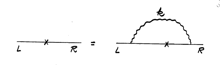
Figure 3: The self energy of quarks with a gluon loop

Using $\gamma^{\mu}D_{\mu\nu}\gamma^{\nu}~{}=~{}-3i/k^{2}$ and a colour factor 4/3 for the colour group SU(3) one gets [6]

$$-m(\rho)~{}=~{}4g_{s}^{2}\frac{m(\rho)}{(2\pi)^{4}}\int d^{4}k[\frac{i}{k^{2}[(p-k)^{2}-m(\rho)^{2}]}-\frac{2\pi\delta[(p-k)^{2}-m(\rho)^{2}}{k^{2}}f(p_{0}-k_{0})]$$ (3)

where we have neglected a Boson finite $T$-term which deos not contribute and $f$ is the Fermi function

$$f(E)=\frac{1}{1+exp[(E-E_{F})/T]}.$$ (4)

In the rest frame, $\vec{p}=0$. The Fermi function becomes a step function for our case, since the temperature T = 0. On closing the contours in the lower half $k_{0}$ plane, first term reduces to

$$\int\frac{d^{3}k}{(2\pi)^{3}}[\frac{1}{2E[(m-E)^{2}-{\vec{k}}^{2}]}-\frac{1}{4m{\vec{k}}^{2}}]=\frac{4g_{s}^{2}m}{8\pi^{2}}\int\frac{dk}{E}$$ (5)

while the second term becomes, on using the variable $p-k\rightarrow q$,

$$4g_{s}^{2}m\int\frac{d^{4}q}{(2\pi)^{2}}\frac{\delta(q^{2}-m(\rho)^{2})}{(p-q)^{2}.(exp[{(q_{0}-\mu)\beta}]+1}=\frac{-4g_{s}^{2}m}{8\pi^{2}}\int\frac{dq}{E}\frac{2}{exp[{(q_{0}-E_{F})\beta}]+1}$$ (6)

$\rho_{B}/\rho_{0}$	$\nu~{}=~{}$	0.333	0.286	0.400
5		0.5093	0.522	0.5156
6		0.5077	0.5025	0.478
7		0.4919	0.4739	0.4384
8		0.4693	0.4427	0.4012
9		0.444	0.412	0.3676
10		0.4185	0.3833	0.3379
11		0.3939	0.3571	0.3119
12		0.3707	0.3334	0.2891
13		0.3493	0.3121	0.2691
14		0.3297	0.2929	0.2516
15		0.3117	0.2758	0.2361
16		0.2953	0.2604	0.2223
17		0.2803	0.2465	0.21
18		0.2666	0.2339	0.199

Table 1: Variation of $\alpha_{s}$ with density for three values of $\nu$

The first integral is logarithmically divergent and therefore must be set to renormalize the $\rho=0,~{}T\equiv 1/beta~{}=0$ quark mass. We do not use a high value of $g_{s}^{2}/4\pi~{}\equiv~{}\alpha_{s}=0.75$ like [6] since it gives a cut-off which is too small, of magnitude $1.29~{}GeV$ only. We prefer a lower $\alpha_{s}=0.55$ and this also gives us a high cut-off $k_{D}~{}=~{}2.86~{}GeV$. We use $m(\rho=0)=0.33~{}GeV.$

   

Figure 4: The figure shows the smooth decrease in the value of the strong coupling constant with the increase of baryonic density. We have plotted three curves corresponding to the three values of the parameter $\nu$ ( = 0.286, 0.333 and 0.040) of eq. (1).

Now we introduce the second term for finite $\rho$ but $T=0$ so that the Fermi function reduces to a step function.

$$m(\rho)=m(0)-\frac{\alpha_{s}}{\pi}\int_{0}^{E_{F}}\frac{dE}{\sqrt{E^{2}-m(\rho)^{2}}}.$$ (7)

Given our form for $m(\rho)$, which is $M_{Q}$ of eq.(1), dropping the current quark mass $m_{i}$, $\alpha_{s}$ is now evaluated for all densities. For small density its value increases but this is unnecessary for our model. We get very reasonable values of $\alpha_{s}$ for $\rho=5\rho_{0}$ upwards as can be seen in Table 1 and also in Fig(4). The calculation serves double purposes, it shows that for the concerned densities our choice of the mass function, namely eq.(1), is reasonable and also as already stressed it gives a novel shape for the variation of $\alpha_{s}$ with density not easy to obtain otherwise.

The variation with $\nu$ is very small at the surface but deep inside the star when the density increases the values of $\alpha_{s}$ goes down substantially and the change assumes significance. The physicality of the results will enable us to extend our calculation now to $T~{}\neq~{}0$ and apply to early universe where temperature of order $100~{}MeV$ is expected.

In summary we have shown both in principle and in practice that the strong coupling constant can be derived at various densities once one knows the behaviour of the chiral symmetry restoration for the quark mass constrained from stellar data. The practical model that we have chosen uses an empirical form for chiral restoration at high density proposed and tested against various star properties through the allowed mass radius regions of the compact objects[1, 2, 3]. We can therefore urge the astrophysics data-analysts to pinpoint the mass and radius of compact objects like SAX J1808.8 to a greater precision to help efforts like ours.

It is a pleasure to thank Dr. Arun Thampan for helpful discussions. The stimulation for the work came from a discussion with Prof. Donald Lynden-Bell.

References

- [1] M. Dey, I. Bombaci, J. Dey, S. Ray and B. C. Samanta, Phys. Lett. B 438, 123 (1998), Addendum B 447 352 (1999) (E) B 467 303.
- [2] X. Li, I. Bombaci, M. Dey, J. Dey and E. P. J. van den Heuvel, Phys. Rev. Lett. 83 3776 (1999).
- [3] X. Li, S. Ray, J. Dey, M. Dey and I. Bombaci, I., Ap. J. 527 L51 (1999).
- [4] M. van der Klis, astro-ph/0001167, submitted to the Annual Review of Astronomy and Astrophysics; to appear September 2000.
- [5] L. Dolan and R. Jackiw, Phys. Rev. D 9, 3320 (1974).
- [6] D. Bailin, J. Cleymans and M. D. Scadron, Phys Rev. D 31, 164 (1985).