NGC1333/IRAS4: A multiple star formation laboratory

Abstract

We present SCUBA observations of the protomultiple system NGC1333/IRAS4 at 450$\mu$m and 850$\mu$m. The 850$\mu$m map shows significant extended emission which is most probably a remnant of the initial cloud core. At 450$\mu$m, the component 4A is seen to have an elongated shape suggestive of a disk. Also we confirm that in addition to the 4A and 4B system, there exists another component 4C, which appears to lie out of the plane of the system and of the extended emission. Deconvolution of the beam reveals a binary companion to IRAS4B. Simple considerations of binary dynamics suggest that this triple 4A-4BI-4BII system is unstable and will probably not survive in its current form. Thus IRAS4 provides evidence that systems can evolve from higher to lower multiplicity as they move towards the main sequence. We construct a map of spectral index from the two wavelengths, and comment on the implications of this for dust evolution and temperature differences across the map. There is evidence that in the region of component 4A the dust has evolved, probably by coagulating into larger or more complex grains. Furthermore, there is evidence from the spectral index maps that dust from this object is being entrained in its associated outflow.

1 Introduction

Stars of all ages are commonly found in binary and multiple systems [1991]. In fact, amongst the youngest stars, the frequency of companions appears to be higher than in older systems (eg Ghez, 1995). In order to understand the initial stages of star formation, we need to understand the initial stages of binary star formation. There have been many theories advanced to explain the formation of binary stars (cf Clarke 1995; Bonnell 1999). These generally include either a fragmentation during collapse [1986, 1991], a fragmentation of a circumstellar disc [1994, 1998] or a post-fragmentation star-disc capture (eg Clarke & Pringle 1991). In order to be able to distinguish between these theories, we need to observe the youngest systems. This paper reports on recent observations of a young, protostellar multiple system NGC 1333 IRAS 4 in order to constrain its formation mechanism.

NGC1333/IRAS4 is a well studied protobinary system. It was first identified as a site of star formation by Haschick et al (1986), who observed two variable H₂O masers. The distinct core was mapped by Jennings et al (1987).

Sandell et al (1991, hereafter SADRR) mapped the system in the submillimetre with UKT14. They confirmed its multiple nature, finding a 30” binary system embedded in diffuse emission. They labelled the components 4A and 4B. Component 4A was seen to be elongated, which SADRR interpreted as a massive disk seen at an oblique angle. Dynamical evidence of binarity for IRAS4 is lacking, but the common envelope of material surrounding the two main components suggests that they are the products of a single collapse event, the extended material being identified as the remnants of the precollapse core. This extended envelope then provides the main motivation for considering IRAS 4 to be a multiple system, rather than a chance superposition of cores.

The system is associated with a high velocity outflow, mapped at various molecular transitions by Blake et al (1995, hereafter BSDGMA). These authors found a high velocity outflow originating from IRAS 4A and aligned with the apparent disk axis.

Minchin et al [1995] measured polarisation at 800$\mu$m for both 4A and 4B. They found that the polarisation position angle was similar for both sources and broadly aligned with the elongated circumbinary emission.

Interferometry by Lay et al [1995] revealed that both 4A and 4B are themselves multiple systems. 4A was revealed to be a binary of separation 1.2” aligned with the direction of elongation of 4A. 4B appeared also to be multiple, but had a more complex nature which could not be determined.

2 Observations

The observations were taken with SCUBA (Submillimetre Common-User Bolometer Array) at the James Clerk Maxwell Telescope on 1997 July 6 about 2 hours after sun rise. ”Jiggle map” data were obtained simultaneously at two wavelengths with SCUBA (Holland et al. 1999) using two hexagonal arrays of 91 bolometers at 450$\mu$m and 37 bolometers at 850$\mu$m with a field of view of about 2.3 arcmin. The total integration time (on+off) was approximately 60 minutes (20 integrations).

The SURF (SCUBA User Reduction Facility; Jenness & Lightfoot 1998) package was used for flat-fielding, extinction correction, sky noise removal, despiking, removal of bad pixels, rebinning and calibration of the images. The sky opacity at zenith was calculated to be 0.38 at 850$\mu$m from skydip observations and 2.1 at 450$\mu$m using the standard extrapolation formula (Jenness et al, in prep). Saturn was used for calibration at 850$\mu$m, resulting in a flux conversion factor of 285 Jy/beam/V, but was too large to be used for 450$\mu$m (no other planet was available), therefore a flux conversion factor of 1200 Jy/beam/V was inferred for the 450$\mu$m observations by examining calibration observations taken at approximately the same time of day from other nights.

3 Morphology of IRAS4 and comparison with earlier results

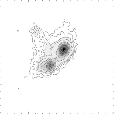
Figure 1: Contour plot of 450$\mu$m jiggle map, overlaid on a greyscale image. The noise is estimated to be approximately 1 Jy/beam, from the RMS deviation about the mean measured in an off source region (marked in Figure 3. The FWHM of the beam is approximately 9”. Contours are drawn at 3, 4, 5, 6, 9, 12, 18, 24, 30, 40, 50 and 60 times the noise level of 0.9Jy/beam. Contours near the peaks have been plotted in white so they can be distinguished from the background. Offsets in RA and Dec are in arcseconds from the peak of 4A, at $\alpha$(2000)=3^h 29^m 10.4^s, $\delta$(2000)=31^o 13${}^{{}^{\prime}}$ 33.6${}^{{}^{\prime\prime}}$

Figure 2: Contour plot and greyscale of 850$\mu$m jiggle map. The noise is estimated to be 0.05 Jy/beam. The FWHM of the beam is approximately 16”. Contours are drawn at 3, 6, 9, 12, 18, 24, 48, 72, 96, 120, 150, 175 and 200 times the noise level. Offsets are measured from the peak of 4A at $\alpha$(2000)=3^h 29^m 10.3^s, $\delta$(2000)=31^o 13${}^{{}^{\prime}}$ 32.9${}^{{}^{\prime\prime}}$

Both jiggle maps are shown as contour plots in Figures 1 and 2. The two distinct components of IRAS4 are clear in both Figures. The main components lie along an axis running NW-SE. The position angle of this axis is approximately 130^o (where position angle is taken to be zero for objects oriented North-South and increases anticlockwise) The position angle of the extended emission surrounding the main system is difficult to determine accurately from the jiggle maps, since the emission region is slightly larger than the size of the map in the long axis direction, and edge effects come into play. However, the direction of elongation is broadly the same as the position angle of the 4A-4B axis. The third knot of emission is visible in both maps, lying some 49 arcseconds to the NE of the 4A-4B axis. This was also noted by SADRR. We will henceforth refer to this as ’4C’.

The peak flux densities we measure from our maps are listed in Table 1, together with values from SADRR for comparison. The errors of SADRR are statisitical errors, taking no account of calibration uncertainties. The errors we quote are RMS deviations from the mean measured in an off-source region (see Figure 3). There will also be considerable calibration uncertainty in both sets of measurements.

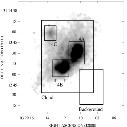
Figure 3: Inverted greyscale plot of raw 450$\mu$m map, with the regions used for photometry for 4A, 4BI, 4BII, and 4C marked. The region used at 850$\mu$m for all 4B is also marked. The region at lower right was used to calculate the background level. The large region covering the whole central part is that used to calculate the extended emission, as discussed in Section 6.1.

At 850$\mu$m and 800$\mu$m the fluxes agree well for source 4A, but not so well for 4B. Since our 850$\mu$m calibration was calibrated reliably, and it is unlikely that such a large discrepency is due to the small difference in the waveband used, we attribute this discrepency to the UKT14 measurements being made one point at a time, with sky conditions and other factors changing during the observations.

At 450$\mu$m the fluxes agree well for source 4B but not for 4A. At this wavelength, calibration inaccuracies for our fluxes could be large. The agreement in flux for source 4B is encouraging, suggesting that our calibration error is likely to be relatively small. Even the 4A flux is not discrepent by as much as a factor of 2. Averaging the discrepencies between the fluxes of these two objects suggests that our calibration error could be around 30%. We note again that the difference in observing technique between UKT14 and SCUBA means that our data is likely to be more internally self-consistent than the UKT14 data since the whole field is observed simultaneously with SCUBA.

450$\mu$m
Object	Peak flux density (Sandell et al.)	Peak flux density (current study)
	(Jy / beam)	Jy / beam
4A	35.6 $\pm$ 4.2	51.03 $\pm$ 1.0
4B	28.0 $\pm$ 5.0	28.04 $\pm$ 1.0
4C	-	5.56 $\pm$ 1.0
850$\mu$m/ 800$\mu$m
4A	10.9 $\pm$ 0.3	10.3 $\pm$ 0.03
4B	5.76 $\pm$ 0.15	4.5 $\pm$ 0.03
4C	-	0.97 $\pm$ 0.03

Table 1: The peak flux densities from our maps, and those found by Sandell et al. (1991). These authors observed at 450$\mu$m and 800$\mu$m using UKT14, with beam sizes of 13.5” HPBW (800$\mu$m) and 7.7” HPBW (450$\mu$m). The chop throw used by Sandell was 60” in both cases. The quoted errors on our values represent the RMS deviation from the mean measured in an off-source region of our maps (marked on Figure 3).

From the 450$\mu$m plot in Figure 1 we can see that 4A itself is significantly elongated, with long axis at a position angle of 154^o, slightly larger than the position axis of 4A-4B. Component 4B is also seen to be elongated, this time in an EW direction.

Interferometric studies (Lay et al, 1995) have revealed that 4A is itself a binary, with separation of 1.2” and position angle aligned with the elongation. The natural interpretation of the large elongated 4A system is that it is a circumbinary disk, foreshortened in the plane of the sky, although from the continuum maps it is possible that it could be an elongated spheroid. We can fit an elliptical Gaussian to 4A and derive the likely inclination angle of the disk. The best fit elliptical Gaussian has position angle 154^o, and ellipticity 0.26, where the ellipticity is defined as $(1-b/a)$, with $a$ and $b$ being the major and semimajor axes respectively. From this we can infer a likely inclination to the plane of the sky of 42^o. The elongation of 4A was also seen by SADRR. They too inferred the presence of a tilted disk and derived a similar apparent inclination to the plane of the sky. The molecular line observations of BSDGMA show bipolar outflows from 4A, whose alignment on the sky and kinematic properties point to them being emitted roughly perpendicular to the plane of this disk. The question of the 4A disk will be addressed again in Section 4.

Lay et al’s interferometry implied that 4B is a multiple system, but they could not determine the exact nature of 4B as the system appeared to be too complex. In both our submillimetre maps, 4B appears extended in an E-W direction. In the 450$\mu$m map this extension is in the form of a small lobe, jutting out from the main part of 4B. This appearance suggests that we may have almost resolved a second component of the 4B system. We will discuss this issue further in Section 4.

4 Richardson-Lucy deconvolution.

The high signal to noise of our maps, together with the existence of high signal to noise planetary maps taken during the same night, allows us to deconvolve the measured SCUBA beam from the data. We did not use our Saturn maps for this, as it is not clear that Saturn is circular in the submillimetre. We instead used high signal-to-noise maps of Uranus taken several hours earlier. We chose to use a Richardson-Lucy technique (Lucy, 1974), as this conserves the flux density. We used a version implemented in the IRAF stsdas package.

4.1 The beam maps

Inspection of the reduced beam maps revealed a departure from circular symmetry at the level of a few percent, with the non-circular part of the beam roughly aligned with the direction of the chop throw (i.e. azimuth). This indicates that the non-circularity due to the chopping dominated over any non-circularity inherent in the array. The beam maps were therefore rotated so that they were azimuthally-aligned with the IRAS4 maps.

The beam maps were apodized by deconvolving a smoothed, circular image, with the radius of Uranus. This removes the planet image from the map, leaving us with just the beam. Both beam maps are shown in Figure 4.

We measured the effective beam area from the Uranus beam maps. The effective area of the 450$\mu$m beam was found to be 110 arcsec², and that of the 850$\mu$m beam was 290 arcsec². The half-power beam widths, measured by fitting circular Gaussians to the beams, were 8.9” and 15.8” for 450$\mu$m and 850$\mu$m respectively. The 850$\mu$m HPBW is therefore consistent with the measured beam area to within a few percent. The 450$\mu$m fitted HPBW implies a beam area of 90 arcsec², 20% smaller than the measured beam area. This gives us an estimate of the effective area of the extended 450$\mu$m error beam.

Figure 4: Contour plots of beam maps, 450$\mu$m (left) and 850$\mu$m (right). The lowest contour at 450$\mu$m is at 10% of the peak flux, the lowest contour at 850$\mu$m is at 2% of the peak flux. These contours show the level of the non-circular part of the beam power. Both beam maps have been rotated to the same azimuthal orientation as the object maps. X and Y axes are in arcseconds.

4.2 Stopping criteria

The decision of when to terminate the deconvolution procedure is of critical importance. Failure to follow the technique far enough results in a non-fully deconvolved map. Following the process too far will result in building noise into apparent structure. Noise levels were measured in regions of the maps judged to best approximate background sky emission. These noise levels could then be specified as a constant noise applied to each pixel, and the deconvolution was terminated when the $\chi^{2}$ calculated for the observed image and the recovered image convolved with the beam reached 1. This convergence criterion was found to be critically dependent on the noise value in the case of the 450$\mu$m map. Values of the RMS deviation about the mean were measured in a region off the cloud and found to range from 0.78 to 1.1 Jy/beam. Noise levels of around 1.0 were found to lead to rapid convergence and an image not significantly improved from the original. Levels as low as 0.95 led to convergence in many iterations, and a final image in which faint structure around IRAS4C had built into peculiar artefacts in the image. We therefore selected a noise level of 0.96. This led to convergence in 48 iterations, and a final image which appeared significantly enhanced compared to the original, but without any apparently artificial structure. It is important to stress that, whilst the assumed noise level was entirely realistic for the 450$\mu$m map, it was eventually selected because it leads to an acceptable deconvolution.

4.3 The deconvolved maps

The results of the deconvolution can be seen in Figure 5. The most striking aspects of these images are the disappearance of much of the circumbinary material, and the resolution of 4B into a binary of separation 12”.

The 850$\mu$m map noise level was estimated similarly and found to be approximately 0.03 Jy/beam. The deconvolved 850$\mu$m map is shown in Figure 6. The deconvolution was again halted when the $\chi^{2}$ reached 1.

Gaussian fits were made to the deconvolved components. The 450$\mu$m image of 4A was found to be well fit by a Gaussian with ellipticity 0.40 and position angle 148.6^o. The greater ellipticity now suggests an inclination of 53^o to the plane of the sky. 4B is seen in the deconvolved maps to consist of two distinct components, which we label BI and BII. A cut across the 4BI-4BII system in the 450$\mu$m map is shown in Figure 7. The separate components of 4B could each be fitted independently. 4BI was found to have an ellipticity of 0.23, implying an inclination angle of 40^o to the plane of the sky. The position angle of 4BI was 140.41^o, aligned much more closely with the position angle of 4A and with the 4A-4B axis, which in the deconvolved 450$\mu$m map was found to be 135^o. This suggests that 4BI may also possess a disk. 4BII was found to have no measurable ellipticity. In each case, deconvolved and raw maps, no evidence for elongation was seen in the case of 4C.

The 4BI-4BII binary is probably too wide (and too simple) to account entirely for the findings of Lay et al (1995). Thus it is likely that either 4BI or 4BII or both are themselves multiple.

Gaussian fitting of the components in the 850$\mu$m deconvolved map revealed no evidence for elongation in the case of 4A. 4B was found to have ellipticity 0.23 with position angle 102^o, which is clearly due to the 4BI - 4BII system being unresolved.

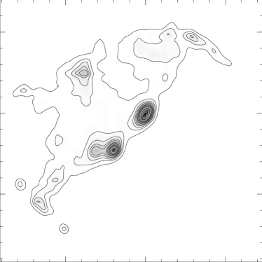
Figure 5: Contour plot of Richardson-Lucy deconvolved 450$\mu$m map, overlaid on a greyscale image. Contours are drawn at 4.5$\times 10^{-3}$, 4.5$\times 10^{-2}$, 0.14, 0.28, 0.41, 0.68, 0.91, 1.4, 2.3, 3.6, 4.5 and 5.5 Jy arcsec^-2.

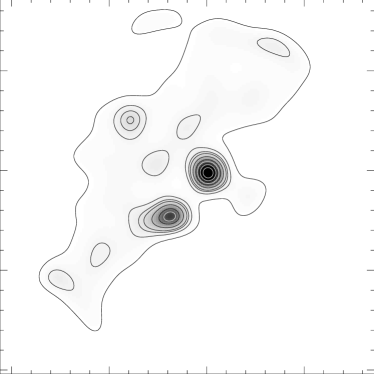
Figure 6: Contour plot of Richardson-Lucy deconvolved 850$\mu$m map. Contour levels are 5$\times 10^{-4}$, 2.6$\times 10^{-3}$, 5$\times 10^{-3}$, 7.8$\times 10^{-3}$, 1.6$\times 10^{-2}$, 0.03, 0.05, 0.06, 0.08 and 0.12 Jy arcsec^-2.

Figure 7: A cut across the deconvolved 450$\mu$m map along the 4BI-4BII axis, connecting the component peaks. The offset in arcseconds is measured from the peak position of component 4BI.

5 Spectral index

With observations at two wavelengths, it is possible in principle to compare the two flux densities and measure the submillimeter spectral index, $\alpha$, point by point across the region of interest. We note first that, since we have assumed our 450$\mu$m flux density conversion factor, the absolute values we derive for the spectral index, and any derived quantities, will be reliant on the accuracy of this assumption. Relative values will still be valid, however, and it is these which we are most interested in.

In practice, the measurement of spectral index is complicated by the uncertain nature of the instrumental beam at 450$\mu$m. In general, the instrumental profile consists of a central Gaussian-type beam, and an extended error beam, which can account for up to half of the effective beam area (See Section 4.1). This will have the systematic effect of reducing the spectral index of compact sources relative to the surrounding cloud. Particular care must therefore be taken when interpreting low values of $\alpha$ for the compact sources as evidence of physical differences, such as temperature or dust evolution effects.

One way to avoid these systematic effects would be to use the deconvolved maps, since the beam pattern will in theory have been removed from these. However, use of the deconvolved maps is not free from systematic effects either. The problems with stopping criteria discussed in Section 4.2 are of particular importance, since the extended emission is quite sensitive to exactly when the deconvolution is terminated.

We therefore believe the best way to calculate spectral indices for the compact sources is to use the photometry presented in Section 6, which was obtained by integrating over appropriate regions in the deconvolved maps calibrated in Jy/arcsec². Values calculated in this way appear in Table 2, together with values of $\beta$ calculated at various temperatures. We have also constructed spectral index maps made from the undeconvolved images, in order to examine the extended structure.

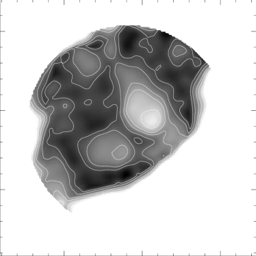
Figure 8: Spectral index map obtained from the raw maps, shown as a greyscale plot with overlaid contours. Contour levels are 3.0, 3.3, 3.5, 3.8, 4.0 and 4.5. The greyscale has been inverted so that regions of higher spectral index appear darker. The x and y axes are arcsec offsets from the position of the peak of 4A. Edge effects have been cut out.

Figure 8 shows the map of spectral index $\alpha$, ($F_{\nu}\propto\nu^{\alpha}$), computed from the raw maps. This map has been recalibrated into Jy/arcsec². The 450$\mu$m map has been degraded to the same resolution as 850$\mu$m. This smoothing is another cause of possible systematic effects, and the correct smoothing was found by minimising the resulting artefacts by a process of trial and error.

The RMS deviation from the mean of the cloud’s spectral index, measured in a region between 4A, 4B and 4C, is 0.08. This value was used as an estimate of the random error in extended regions of the spectral index map.

The compact sources are seen in Figure 8 to have lower spectral index than the surrounding material. Values of $\alpha$ for the sources in the SI map are typically 3 for 4A or 3.5 for 4B and 4C, compared to 4.1 for the cloud.

A region of low spectral index is seen extending from 4A, roughly perpendicular to the 4A disk axis. This region corresponds to the outflow seen in molecular line emission by BSDGMA. The difference in $\alpha$ between the outflow region and the surrounding cloud is approximately 0.5, and is therefore significant compared to the RMS error for the cloud. Since the outflow is not a compact source, it is difficult to see how beam effects could have produced this result. We conclude that the 4A outflow has a lower spectral index than the surrounding cloud.

Computing values for $\alpha$ from the photometry of Section 6, and comparing these to values measured for the cloud from the SI map discussed above, we see again that 4A has a significantly lower $\alpha$ than the cloud. The 4B $\alpha$ is comparable to the cloud, and 4C is even a little higher. This gives us more confidence that the 4A spectral index is genuinely low, but lends no support to the idea that 4B or 4C have significantly lower spectral index than the cloud.

Below, we discuss the various physical causes which could give rise to these spectral index variations.

Object	$\alpha$	$\beta$, (T=20K)	$\beta$, (T=30K)	$\beta$, (T=50K)	$\beta$, (T=100K)
Cloud	4.1∗	2.8	2.5	2.3	2.2
4A	3.7	2.4	2.1	1.9	1.8
4A SW-NE	3.6∗	2.3	2.0	1.8	1.7
4B (I + II)	3.9	2.6	2.3	2.1	2.0
4C	4.4	3.1	2.9	2.7	2.5

Table 2: Values of spectral index, $\alpha$, for different objects and regions in the raw spectral index map. Values for the compact sources are computed from the aperture photometry of the deconvolved maps presented in Section 6, except those marked ^∗ which are mean values found from regions of the raw maps. In the case of the cloud, this region is a square lying near the centre of the field between the three main sources and the outflow. Values of $\beta$ are derived based on the assumption that the emission is optically thin, using various values of the temperature. Values subsequently used to calculate masses in Tables 3 and 4 are highlighted in bold.

Temperature

Provided we assume the emission is optically thin, we can write the spectral index as $\alpha=2+\beta+\gamma$, where $\beta$ is the dust opacity spectral index and $\gamma$ is a factor taking account of the departure from the Rayleigh-Jeans law at low temperatures, which is always negative and becomes significant for temperatures below about 50K. We have taken account of this correction when calculating the $\beta$ values presented in the various tables and used in Section 6.

The temperature of the IRAS4 sources was estimated by SADRR to be 33K, based on a fit to the SED measured at millimetre and submillimetre wavelengths. A temperature of around 30K therefore seems most likely for the compact sources. The gas temperatures were estimated by BSDGMA from their molecular line data, and lie in the range 20-40K for the compact sources, and 70-100K for the wings (the outflow). The surrounding cloud temperature is not estimated, but is likely to lie in between these two values. To illustrate the effects of different temperatures, we have calculated $\beta$ for several different cases, and we have used temperatures of 50K and 100K when calculating the cloud mass.

The difference in $\alpha$ between 4A and the cloud is 0.4. To account for this solely by a difference in temperature, the cloud would need a temperature of approximately 100K if 4A has a temperature of 30K, or 50K if 4A has a temperature of 20K. Thus it is possible to explain the difference in spectral index for 4A as a temperature effect, but this requires a lower temperature for 4A than SADRR determined, or a cloud temperature similar to the temperature in the outflow. The difference in $\alpha$ between the outflow and the cloud is unlikely to be due to temperature, since the outflow is unlikely to be significantly cooler than the cloud.

Optical depth

Determination of spectral indices, and also inferences about the system’s mass, depend on the emission being optically thin. We can investigate the validity of this assumption to some extent by calculating lower limits for the optical depth at each source. This is done by comparing the flux density observed to that expected from a blackbody at an assumed temperature (see e.g. Visser et al, 1998). For reasonable temperatures in the range 20-100K at 450$\mu$m the optical depth at the position of the peak of 4A is at least 0.09. At 850$\mu$m, the peak of 4A has $\tau_{\nu}\geq 0.02$. There is therefore no evidence that our assumption of low optical depth is invalid.

Line contamination

The principal components, and the outflow, are molecular line emission sources (BSDGMA, Lefloch et al, 1998). Contamination of the 850$\mu$m band by line emission, particularly CO 3-2 at 870$\mu$m, could lead to lower spectral index in these regions. We can investigate this possibility by converting BSDGMA’s integrated brightness temperatures for the sources into flux densities. The integrated brightness temperature of the CO 3-2 line is given as 135.4 K km s^-1 for 4A and 64.2 K km s^-1 for 4B. Converting this to a flux density expected in the SCUBA 850$\mu$m beam (assumed bandwidth=30GHz) gives 82mJy/beam for 4A and 39mJy for 4B. This corresponds to 1% (4A) or 2% (4B) of the 850$\mu$m flux density seen in our maps. This would lead to a spectral index lower by 0.01 or 0.02, not alone sufficient to explain the spectral index deficits observed for the compact sources. Summing the integrated intensities for all the lines in the SCUBA 850$\mu$m band gives a total value of 150 K kms^-1, still not sufficient to explain the low spectral index of the compact sources. The outflow region may be more susceptible to line flux contamination, as the dust continuum emission is lower. Typical integrated line intensities measured by BSDGMA in this region are of order 6-10K km s^-1, corresponding to a flux level of perhaps 6 mJy/beam out of a typical continuum flux of 0.8Jy/beam in this region in the 850$\mu$m map. This is less than 1% of the continuum flux level and so also unlikely to lead to a significantly lower spectral index.

It should be noted that the contamination of the 850$\mu$m band by CO 3-2 will be offset by the contamination of the 450$\mu$m band by the CO 6-5 line. Assuming CO 6-5 is a factor of 2 stronger than the 3-2 line (as expected if the temperature is of order 100K), the expected spectral index dip is of order 0.005 for 4A, and the expected spectral index dip for the other sources is then also reduced.

Finally, we note that there is no detectable evidence of the outflow as a brighter region in the raw 850$\mu$m map or as a less bright region in the raw 450$\mu$m map. There is an area of low emission in the outflow region in the deconvolved 450$\mu$m image (Figure 5), and of extra emission to the southwest of 4A at 850$\mu$m. The 450$\mu$m gap could well be due to a tendency for the Richardson-Lucy algorithm to build flux density towards the compact sources, thus clearing a gap. It is to avoid uncertainties such as this that we have constructed the SI map from the raw rather than the deconvolved maps.

Dust opacity index

If we can discount the preceding causes of varying $\alpha$, we are left with the possibility that a variation in the dust opacity index $\beta$ is responsible. This would then indicate differing dust properties across the map. Lower $\beta$ can be caused by larger dust grains, indicating that grain growth has occurred in regions of lower spectral index. Alternatively, grain evolution from roughly spherical to more needle-like shapes or to fluffy fractal-like structures could have the effect of lowering $\beta$. Chemical evolution is also possible. See for example Ossenkopf & Henning (1994) or Pollack et al (1994) for discussions of spectral index properies of evolving grains, or Dent et al (1998) for an extensive set of observations of young stellar objects.

The cloud in general seems to have $\beta\sim 2.3$, whilst the outflow region has $\beta\sim 1.8$. It slightly surprising that the region of the outflow should have such a low spectral index. We have already argued that line contamination alone is unlikely to explain this, whilst drastically lower temperature in the outflow seems highly unlikely. We suggest that dust from the region of 4A is swept up and entrained in the outflow.

6 Photometry and masses

Provided the emission is optically thin at some frequency $\nu$, the dust mass of an object can be estimated by

$$M_{d}\approx\frac{F_{\nu}D^{2}}{\kappa_{\nu}B_{\nu}(T)}$$ (1)

(Hildebrand, 1983), where $F_{\nu}$ is the observed flux density, $D$ is the distance, $B_{\nu}(T)$ is the Planck function for a particular temperature, and $\kappa_{\nu}$ is the dust emissivity, given by

$$\kappa=0.1\left(\frac{250}{\lambda(\mu m)}\right)^{\beta}{\rm cm^{2}g^{-1}},$$ (2)

which we have taken from Beckwith & Sargent (1991). Here, $\beta$ is the dust opacity index, discussed above in Section 5. The distance to IRAS4 is approximately 350pc (Herbig & Jones, 1983).

We determined flux density levels from the deconvolved maps, by integrating flux density within the areas indicated in Figure 3 (the box over 4B was split into two when measuring the flux density levels of 4BI and 4BII in the 450$\mu$m map). The flux densities were calibrated in Jy/arcsec², using the measured effective beam areas as discussed in Section 5.

We estimate the masses of the compact objects using an assumed temperature of 30K and corresponding values of $\beta$ as listed in Table 2. The results for the compact components are shown in Table 3.

Wavelength	Object	Flux density (Jy)	$\beta$	Mass ($M_{\odot}$)
450	4A,	139.0$\pm 2.7$	2.1	11.5${}^{+0.5}_{-0.5}$
	4BI,	62.5$\pm 2.2$	2.3	5.8${}^{+0.3}_{-0.3}$
	4BII,	16.4$\pm 0.6$	2.3	1.5${}^{+0.1}_{-0.07}$
	4C,	21.2$\pm 3.8$	2.9	2.8${}^{+0.4}_{-0.4}$
850	4A,	12.9$\pm 0.04$	2.1	10.9${}^{+1.1}_{-1.0}$
	4B,	6.4$\pm 0.05$	2.3	6.9${}^{+0.7}_{-0.7}$
	4C,	1.3$\pm 0.04$	2.9	2.9${}^{+0.3}_{-0.3}$

Table 3: Dust masses derived from the photometry for the compact sources. Total flux densities are measured by integrating the flux density within an aperture - see Figure 3 for the apertures used in the case of 450$\mu$m. The temperature is assumed to be 30K in each case. Source 4B has been considered as two separate sources at 450$\mu$m, but not at 850$\mu$m. Quoted errors for the flux densities are the same percentage error for each source as the flux density error in Table 1, and so contain no estimate of calibration uncertainties, uncertainties due to the choice of aperture, etc. Errors for the masses are a combination of the photometric errors, and an error of $\pm$0.08 in the dust opacity index $\beta$, as measured from the cloud region between the compact sources. Note that although the real error in the absolute value of $\beta$ is larger than this, it is not independent of the assumed temperature. The spectral index uncertainty usually dominates, particularly at 850$\mu$m. The variation due to different assumptions of temperature is considerable. For example, adopting an alternative temperature of 50K would lead to a reduction in the derived masses by a factor of approximately 2.

6.1 Extended emission

Estimating the mass of the extended emission is problematic. For a start, the cloud extends beyond the edges of the jiggle maps, so a direct measurement of the total cloud emission and mass is impossible. Another problem arises from the danger that parts of the map may chop onto other parts. The chop direction is approximately in the $\pm$ RA direction, and the throw is 120”. Thus the central regions should chop onto regions away from the extended ridge. The areas at upper right and lower left may well be affected by chopping onto significant emission, however.

$\lambda$	Flux density	T	$\beta$	Mass (M${}_{\odot})$
450	47.5$\pm 5.2$	50	2.3	2.1$\pm 0.3$
		100	2.1	0.78$\pm 0.09$
850	7.73$\pm 0.08$	50	2.3	4.4$\pm 0.5$
		100	2.1	1.6$\pm 0.2$

Table 4: Cloud masses for different assumptions of temperature and corresponding $\beta$ at 450$\mu$m and 850$\mu$m. Photometric errors are calculated based on the measured background RMS deviation from the mean, and include contributions from the uncertainties in the subtracted core flux densities. Errors for the masses also include the effect of a $\pm 0.08$ random error in the opacity index $\beta$.

We can make a measurement of the extended flux density in the maps, in order to produce a lower limit to the total mass of the surrounding cloud. This was done by summing the emission over the central part of the map (shown in Figure 3) and subtracting the flux already determined for the compact sources. Table 4 shows the masses calculated from the extended emission at 450$\mu$m and 850$\mu$m for various assumed parameters. These masses are considerable, representing about half the mass of the system. The 850$\mu$m mass estimates are about a factor of 2 greater than those at 450$\mu$m.

6.2 Mass ratios

Calculating mass ratios at 450$\mu$m and 850$\mu$m from the data in Table 3 and averaging, we obtain;

$$\frac{4BI+4BII}{4A}=0.63,$$ (3)

and

$$\frac{4C}{4A+4BI+4BII}=0.15.$$ (4)

The ratio for the 4BI - 4BII system, measured from the 450$\mu$m map only, is

$$\frac{4BII}{4BI}=0.26.$$ (5)

7 Discussion

Morphology of IRAS4

The elongation of 4A could be explained as a circular disk inclined at an angle of approximately 53^o to the plane of the sky. The elongation of 4B in the raw map appears to be EW. However, upon deconvolving the beam from the map we discovered that this elongation is due to 4B being itself a binary system. The primary component of 4B in the deconvolved 450$\mu$m map appears to have a slight elongation along the same axis as 4A.

The amount of diffuse material in which the system is embedded is difficult to determine with any accuracy, since the map does not encompass the entire extended ridge, the flux density levels may be affected by the chop throw sampling some of the extended emission, and at 450$\mu$m the error beam may spread flux density from the compact sources into the surrounding regions.

Stability of the system

The separation of the 4B double is approximately 12” on the sky. If we assume that the triple system is coplanar, so that the 4BI-BII axis has the same inclination to the plane of the sky as the 4A disk, the true BI-BII separation would then be 16” (5600 AU for a distance of 350pc). The 4A-4B separation is approximately 30”. The long axis of the 4A disk extends some 8” from the centre in the deconvolved images (we measure the disk extent as the distance at which the flux density reaches 5% of its peak value). Thus the presence of the 4A disk is not incompatible with the interpretation that 4A, 4BI and 4BII have coplanar orbits.

We can also make an assessment of how stable the triple 4A-4BI-4BII system is. We first assume that the system is coplanar and the orbits circular. A criterion for stability in a hierarchical triple was developed by Harrington (1977),

$$\frac{D_{triple}}{D_{binary}}>K\left\{1+A\ln\left[\frac{2}{3}\left(1+\frac{M_{3}}{M_{1}+M_{2}}\right)\right]\right\}.$$ (6)

Here, $D_{triple}$ is the periastron distance of the stand-alone star, and $D_{binary}$ the semi-major axis of the binary orbit. $M_{3}$ is the mass of the single component, $M_{1}$ and $M_{2}$ the masses of the binary components. The constants have values $K=3.5$ and $A=0.7$ for a corevolving system, or $K=2.75$, $A=0.64$ for a counterrotating system. For our case, the mass ratio is $1/0.63$ (Section 6.2). The semimajor axis of the BI-BII system cannot be smaller than the observed separation on the sky of 12”. The true 4A-4BI separation of course depends on the angle of the binary-single star axis. We have already argued (as have previous authors) that the 4A elongation is an inclined disk. If we assume that the 4A-4BI orbit is coplanar with the 4A disk (expected if fragmentation formation models apply), then the true 4A-4BI distance would be 30”, which would also be the largest possible periastron distance. Taking these figures we find that the system fails Harrington’s stability test easily, even if we consider the more stable counterrotating case. See Figure 9.

Figure 9: Harrington’s stability test as applied to IRAS4. The x-axis is the mass ratio $M_{3}/(M_{1}+M_{2})$. The y-axis is the ratio of periastron distance to binary separation. The two bold lines represent the corotating and counterrotating stability limits. The lower of the two represents the more stable counterrotating case. Systems above these lines will be stable. The position of the 4A-4BI-4BII system is marked as a point. The error in the mass ratio is calculated from the errors in Table 3. The uncertainty in the ordinate has been estimated as follows. The misalignment between component BI and the axis of elongation of 4A was projected back into the plane of the supposed 4A disk. This then gives the possible discrepency between the 4A-4BI distance measured in the plane of the sky and the inferred 4A-4BI distance in the plane of the disk. The upper error bar shows the possible increase in stability due to this observed misalignment. Since the quantities $D_{triple}$ and $D_{bin}$ have been chosen to maximise stability, the y-position of the IRAS4 system is an upper limit.

It is possible to envisage accretion of material stabilising initially-unstable triple systems by modifying the separation ratios of the components (Smith et al, 1997). There certainly seems to be a substantial reservoir of available material in the IRAS4 envelope (see Table 4). In the case of a low-mass binary orbiting a higher-mass single star, as here, this mechanism is unlikely to result in stability. Low specific angular momentum material will tend to be accreted onto IRAS4A, causing the single-binary separation to decrease and destabilizing the system. High specific angular momentum will tend to accrete onto the binary (4BI-4BII), widening it by adding angular momentum and again destabilizing the system. Furthermore, the 4A-4BI-4BII system fails the Harrington stability test by a comfortable margin. Even if the available envelope mass were accreted exclusively onto 4BI and BII, moving the mass ratio towards 1, there is not enough mass to entirely stabilize the system. We conclude that IRAS4 seems to be an unstable multiple which will be disrupted within a few orbits.

Star forming history of IRAS4

Could the elongation of the main cloud be explained as a foreshortened disk, in a similar way to the elongation of 4A? The young age (approx 10⁵ years deduced from the embedded nature), appears to preclude this interpretation. For a circumstellar disk to form requires several of the disks dynamical time and a disk of this size would have a period in excess of 4$\times$10⁵ years. This implies that the extended structure must be a remnant of the cloud’s initial conditions and not due to the subsequent collapse dynamics.

Based on their polarimetric observations, Minchin et al suggested that the extended emission is an inclined “pseudo-disk”, of the sort envisaged by for example Galli & Shu (1993). In this case, the cloud material is magnetically supported in one direction, but free to collapse in the other. A massive, non-centrifugally supported disk can therefore form in a shorter time than would be expected on dynamical grounds. The ambipolar diffusion timescale would have to be longer than the freefall time of the cloud, and the magnetic field would be an impediment to fragmentation of the central region, because it would tend to enforce solid body rotation. For this reason, we do not favour the “pseudo-disk” interpretation.

Simulations indicate that a prolate cloud, with an end-over-end rotation, should undergo fragmentation and form a central binary (Bonnell et al, 1992, Bonnell & Bastian 1992). The additional multiplicity of the system (4BI-4BII) is then explainable as being due to an internal disk fragmentation (Bonnell 1994) that occurs in the individual components formed in the prolate cloud fragmentation (Bonnell et al 1992). This interpretation still leaves us with some unexplained details. Most importantly, the third component to the north east. There are several possible explanations for this component. Firstly, it could be part of the IRAS 4 system, but lie outside of the prolate cloud, in front of the main system and well above the plane of the IRAS 4A disk and inferred 4A-4B orbit. This poses substantial problems for fragmentation models where collapse occurs preferentially in one direction, reducing the dimension of the cloud and making it unstable to fragmentation (Bonnell 1999). Secondly, it could lie in the same plane as the 4A disk, which would place it well outside the prolate cloud as it is seen in the maps, at a distance of 15,400 AU (44” at 350pc).

If IRAS 4C is part of the IRAS 4 system, then the most promising explanation is that an independent condensation (see eg, Pringle 1991) was present near the prolate cloud when collapse occured.

There exists the possibility that IRAS 4C is not a member of the IRAS 4 system but just a chance projection. Its separation and the presence of other sources nearby lend credence to this possibility, as does it’s spectral index being higher than the surrounding cloud. A determination of the velocities of the various components could shed further light on the possible relationship of 4C with the central system.

8 Summary

We have examined high signal to noise maps of the protostellar multiple system NGC1333/IRAS4. We have estimated the masses of the principle components, and discussed the probable configuration, possible history, and likely future of the system on dynamical grounds. In the light of fragmentation models of binary formation, we argued that the elongated geometry of the main cloud is probably due to a prolate rather than disk-like geometry, because magnetically-supported flattened structures are not expected to undergo fragmentation to form a multiple system such as IRAS4. The third major component, 4C, poses problems for any almost any model as it lies either too far from the central system, or out of the plane of the main binary orbit. We suggest that 4C may be an independent condensation in the cloud. By comparing the masses and separations of the central triple system, assuming coplanarity, we showed that it is clearly not stable. Thus IRAS4 is an example of a multiple system which has formed from fragmentation of a tumbling prolate cloud, but which is will in future disintegrate to leave fewer, lower order multiple or single systems.

We constructed a map of spectral index for the system. Despite the various problems associated with the measurement of this quantity, we concluded that there is marginally significant evidence that 4A has a low spectral index compared to the cloud. There is also strong evidence that the region associated with the 4A outflow has a low spectral index. Various possible causes of this were discussed. There is no evidence suggesting that the emission is optically thick at either wavelength. The apparently low spectral index of 4A was dependent on temperature assumptions, but the outflow region should not be systematically cooler than the surrounding cloud, so this is unlikely to provide an explanation. We considered the possibility that molecular line emission could manifest itself as a region of low spectral index by contaminating the 850$\mu$m flux density. Based on the measured line strengths from BSDGMA, this explanation seemed unlikely to be the sole cause, although it could constitute a partial cause. It was therefore concluded that the low spectral index of 4A was most likely an indication of dust grain growth in the dense circumstellar disks. This grain growth then appears to be more advanced in 4A than in 4B or 4C.

We have seen an area of low spectral index running through IRAS4A, in the position of the molecular outflow seen by BSDGMA. This ridge is seen on both sides of IRAS4A, and is clearly distinct from IRAS 4C to the Northeast. We argued in Section 5 that contamination from molecular line flux is probably not sufficient to explain this. We suggest the possibility that dust from the vicinity of IRAS4A is being swept up and entrained in the outflow. This suggests models in which the driving mechanism for the outflow is a jet embedded in the protostellar core itself (see e.g. Masson & Chernin 1993; Chernin et al 1994; Raga & Cabrit, 1993). If this explanation is correct, the main issues for outflow theories would seem to be that the driving mechanism should not be so violent that dust grains are destroyed in large numbers, and that significant amounts of dust material should occupy the outflow cavity after the main jet working surfaces have passed through.

9 Acknowledgements

The JCMT is operated by the Joint Astronomy Centre, on behalf of the UK Particle Physics and Astronomy Research Council, the Netherlands Organization for Pure Research, and the National Research Council of Canada. The authors thank James Deane and Jane Greaves for helpful discussions and advice.

References

- [1991] Beckwith S.V.W. & Sargent A.I., 1991, ApJ 381, 250
- [1995] Blake G.A., Sandell G., van Dishoeck E.F., Groesbeck T.D., Mundy L.G. & Aspin C., 1995, ApJ 441, 689 (BSDGMA).
- [1998] Boffin, H. M. J., Watkins, S. J., Bhattal, A. S., Francis, N. & Whitworth, A. P., 1998 MNRAS 300, 1189
- [1991] Bonnell I.A., Martel, H., Bastien P., Arcoragi, J.-P., Benz, W., 1991, ApJ 377 553
- [1992] Bonnell I.A., Arcoragi, J.-P., Martel, H. & Bastien, P., 1992, ApJ 400 579
- [1992] Bonnell I.A. & Bastien P., 1992, ApJ 401 654
- [1994] Bonnell I.A., 1994, MNRAS 269, 837
- [1999] Bonnell, I. A., 1999, in The Origin of Stars and Planetary Systems, C. Lada and N. Kyfalis (eds),(Kluwer) p. 479.
- [1986] Boss A.P., 1986, ApJS 62, 519
- [1994] Chernin L.M., Masson C.R., Gouveia dal Pino, E.M. & Benz, W. 1994, ApJ 426, 204.
- [1991] Clarke C.J. & Pringle J.E., 1991, MNRAS 249, 584
- [1995] Clarke C.J., 1995 in Evolutionary Processes in Binary Stars, eds R. Wijers, M. Davies, C. Tout, Kluwer Academic, p. 31
- [1998] Dent W.R.F., Matthews H.E., & Ward-Thompson D., 1998, MNRAS 301, 1049
- [1991] Duquenney & Mayor, 1991, A&A 248, 485
- [1993] Galli D. & Shu F.S., 1993, ApJ 417, 220
- [1995] Ghez A., 1995, in Evolutionary Processes in Binary Stars, eds R. Wijers, M. Davies, C. Tout, Kluwer Academic, p. 1
- [1977] Harrington R.S., 1977, AJ 82, 753
- [1986] Haschick A.D., Moran J.M., Rodriguez L.F., Burke B.F., Greenfield P. & Garcia-Barreto J.A., 1986, ApJ 237, 26
- [1983] Herbig G.H. & Jones B.F., 1983, AJ 88, 1040
- [1983] Hildebrand R.H., 1983, QJRAS 24, 267
- [1999] Holland W.S. et al, 1999, MNRAS, 303, 659
- [1998] Jenness T., Lightfoot J.F., 1998, Astronomical Data Analysis Software and Systems VII, A.S.P. Conference Series, Vol. 145, 1998, R. Albrecht, R.N. Hook and H.A. Bushouse, eds., p.216
- [1987] Jennings R.E., Cameron D.H.M., Cudlip W. & Hirst C.J., 1987, MNRAS 226, 461.
- [1995] Lay O.P., Carlstrom J.E. & Hills R.E. 1995, ApJ 452, L73.
- [1998] Lefloch B., Castets A., Cernicharo J. & Loinard L., 1998, ApJ 504, L109.
- [1974] Lucy L.B., 1974, AJ 79, 745
- [1993] Masson C.R. & Chernin L.M., 1993, ApJ 414, 230.
- [1995] Minchin N.R., Sandell G. & Murray A.G. 1995, A&A 293, L61.
- [1994] Ossenkopf V. & Henning T., 1994, A&A 291, 943.
- [1994] Pollack J.B., Hollenbach D., Beckwith S., Simonelli D.P., Roush T., & Fong W., 1994, ApJ 421, 615
- [1991] Pringle J.E., 1991, in The Physics of Star formation and early stellar evolution, eds C. Lada and N. Kylafis, Kluwer, pg 437 - 448
- [1993] Raga A. & Cabrit S., 1993, A&A 278, 267
- [1991] Sandell G., Aspin C., Duncan W.D., Russell A.P.G., & Robson E.I., 1991, ApJ 376, L17 (SADRR)
- [1997] Smith K.W., Bonnell I.A. & Bate M.R., 1996, MNRAS 288, 1041
- [1998] Visser A.E., Richer J.S., Chandler C.J. & Padman R., 1998, MNRAS 301, 585