Cluster Detection in Astronomical Databases: the Adaptive Matched Filter Algorithm and Implementation

Abstract

Clusters of galaxies are the most massive objects in the Universe and mapping their location is an important astronomical problem. This paper describes an algorithm (based on statistical signal processing methods), a software architecture (based on a hybrid layered approach) and a parallelization scheme (based on a client/server model) for finding clusters of galaxies in large astronomical databases. The Adaptive Matched Filter (AMF) algorithm presented here identifies clusters by finding the peaks in a cluster likelihood map generated by convolving a galaxy survey with a filter based on a cluster model and a background model. The method has proved successful in identifying clusters in real and simulated data. The implementation is flexible and readily executed in parallel on a network of workstations.

1 Introduction

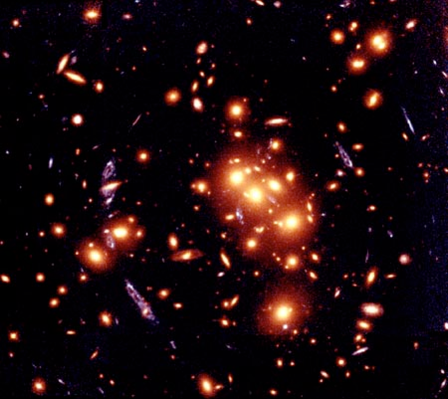
Figure 1: Cluster Image. The cluster 0024+1654 as seen with the Hubble Space Telescope [Colley et al 1996]. The reddish circular patches in the center are Spheroidal galaxies each containing $10^{12}$ stars. The flatter reddish patches are Spiral galaxies like our own Milky Way. The blue arcs around the edge are from a distant background galaxy that has been gravitationally ”lensed” by the cluster. This cluster has around one thousand members and lies at a distance of 4.5 billion light years. [Note: our nearest neighbor the Andromeda galaxy is 1.5 million light years away.]

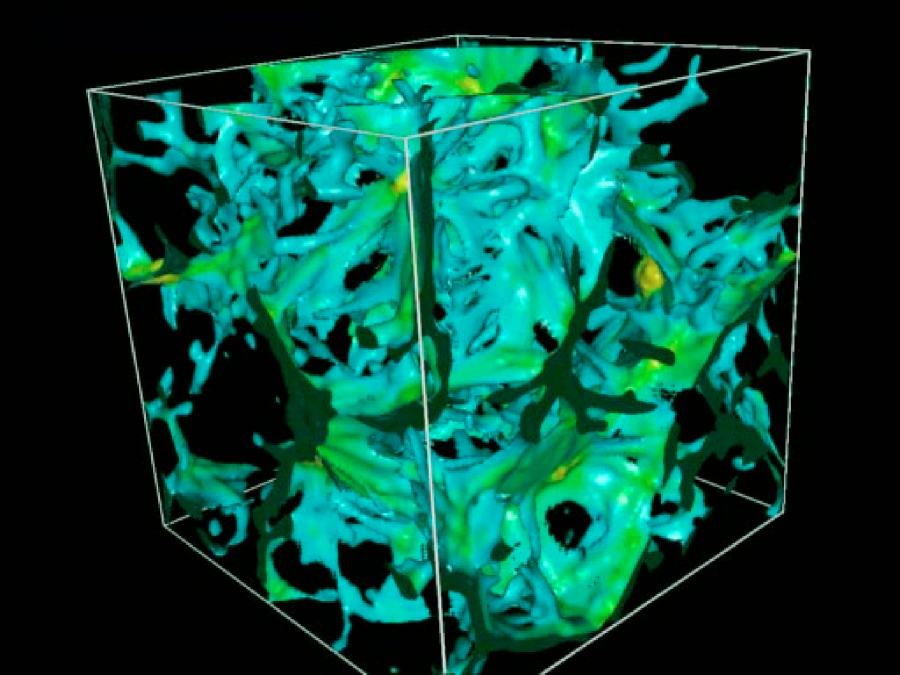
Figure 2: Filament Simulation. Isosurface view of a 3D simulation (courtesy of Michael Norman) of the Universe showing the sheets and filaments of matter along which galaxies form. Clusters of galaxies tend to form where two filaments cross. The simulation volume is approximately 500 light years on a side.

Clusters of galaxies are the largest objects known to humans (see Figure 1). They are the “mountains” of the Cosmos, and like terrestial mountains they lie in great ranges that define the cosmic “continents” and “oceans” (see Figure 2). Mapping clusters of galaxies is very much akin to surveying our own world and allows us to understand the creation, evolution and eventual fate of our Universe [Bahcall 1988].

The process by which astronomers detect clusters of galaxies begins with assembling large images of the sky, which are the result of hundreds of nights of observing through a telescope. These pictures are analyzed to produce a database of galaxies $X=\{{\bf x}_{i}:i=1,\ldots,N_{X}\}$, where $N_{X}\sim 10^{8}$. Each record ${\bf x}_{i}\in X$ consists of a position on the sky, brightness measurements in one or more bands and possibly hundreds of additional measurements describing the shape and composition of the galaxy.

Clusters are local density peaks in the three dimensional distribution of galaxies across the Universe. In 3D data, clusters are easy to detect. Unfortunately, the majority of distances to individual galaxies are not known and can only be inferred statistically from empirical models of their brightness. Thus, it is difficult to differentiate small nearby clusters from large far away clusters. The goal of cluster detection and estimation is to create a catalog, $\Theta$, consisting of thousands of clusters $\Theta=\{{\bf\theta}_{i}:i=1,\ldots,N_{\Theta}\}$, where $N_{\Theta}\sim 10^{4}$. Each cluster in this list, ${\bf\theta}_{i}$, consists of a position on the sky, a distance estimate, a size estimate and perhaps additional estimated properties of the cluster.

The first catalog of galaxy clusters was compiled by Abell [Abell (1958)], and has proved extremely useful to astronomers over the past four decades. Abell’s catalog was created by visually inspecting hundreds of photographic plates taken from the first Palomar Observatory Sky Survey (POSS). Modern galaxy databases are too large for such methods to be used today. Subsequent efforts to detect clusters have relied on Matched Filter techniques taken from statistical signal processing (e.g., [Lumsden et al 1992], [Dalton et al 1994], [Postman et al 1996], [Kawasaki et al 1997] and [Bramel et al 2000]. These methods have a strong mathematical foundation, but require extensive prior information and are often computationally prohibitive as they test every possible location in the domain of the cluster space $\Omega_{\Theta}$ for the presence of a cluster. The Adaptive Matched Filter [Kepner et al 1999] that is described later in this paper is a variation on the Matched Filter that uses a hierarchical set of filters, as well as software coding and parallel computing techniques that address some of the Matched Filter’s drawbacks. The AMF is adaptive in two ways. First, the AMF uses a two step approach that first applies a coarse filter to find the clusters and then a fine filter to provide more precise estimates of the distance and size of each cluster. Second, the AMF uses the location of the data points as a “naturally” adaptive grid to ensure sufficient spatial resolution.

A variety of other techniques have also been applied to the cluster finding problem. The compact nature of clusters make Wavelet based signal processing approaches an appealing alternative [Fan & Pando 1997] and [Fadda et al 1997]. Geometric approaches such as Voronoi tessellation [Ramella 1998] have also been used. In this method each ${\bf x}_{i}$ is the seed for the tessellation. Clusters are then found by computing the volume of each tessel and selecting the points with the smallest volume, which presumably have the highest density. Such geometric methods have the advantage that they require very little prior information.

The Matched Filter, Adaptive Matched Filter, Wavelet and Voronoi Tessellation approaches all use the three to five high affinity dimensions of $X$ (i.e., angular position and brightness measurements). These dimensions are continuous real variables that lend themselves to Euclidean distance metrics. Working in these lower dimensions allows more compute intensive techniques which are necessary to de-project clusters from the observed data domain $\Omega_{X}$ to the desired underlying domain in which clusters exist $\Omega_{\Theta}$, i.e., angular position, distance and size. More recently, there has been interest in exploiting the low affinity dimensions that are also available in galaxy databases [Djorgovski et al 1997, Gal et al 1999] to enhance detection. As the understanding of these methods increases, the exploitation of many dimensions should be possible using advanced datamining techniques (see e.g. [Fayyad et al 1996] and [Dasarathy 1999] and references therein). These methods have enormous potential for detecting new clusters and possibly separating them into distinct groups thus revealing new classes of galaxy clusters.

The rest of this paper presents in greater detail the AMF algorithm, its implementation and results. In section two a detailed derivation of the AMF is given. The derivation is meant to be sufficiently general that it can lend itself to other types of databases. Section three presents the implementation of the AMF using a layered software architecture and a client/server parallelization model. Again, these methods are not limited to the specific problem presented here and are applicable to a variety areas. In section four the results of applying the AMF on simulated and real data are discussed. Finally, section five gives the summary and conclusions.

2 Adaptive Matched Filter Algorithm

Matched filter techniques are widely used in statistical signal processing. The idea is to convolve the data with a model of the desired signal. In many instances this can be shown to be optimal detection method in the least squares sense. Applying matched filter techniques to point set data is less common but has become the standard method for detecting cluster of galaxies. The advantage of matched filter techniques is that they are mathematically rigorous, provide well defined selection criteria and produce few false detections.

The Adaptive Matched Filter [Kepner et al 1999] enhances the matched filter method by creating a pair of filters (each correct under own its assumptions) which can be used to trade off computational complexity versus sensitivity. The filters are derived by computing the likelihood a cluster exists at a particular point ${\bf\theta}\in\Omega_{\Theta}$ given the data $X$. Various likelihood functions can be derived; the differences are due to the additional assumptions that are made about the distribution of the data. This section gives the mathematical derivation of the two likelihood functions used in the AMF: ${\cal L}_{\rm coarse}$ and ${\cal L}_{\rm fine}$. Both derivations are conceptually based on virtually binning the data, but make different assumptions about the distribution of points in the virtual bins.

Imagine dividing up the data domain $\Omega_{X}$ into bins. We assign to each bin a unique index $j$. The expected number of data points in bin $j$ given that their is a cluster at ${\bf\theta}$ is denoted $n_{\rm model}^{j}({\bf\theta})$. The number of data points actually found in bin $j$ is $n_{\rm data}^{j}$. In general, the probability of finding $n_{\rm data}^{j}$ points in cell $j$ is given by a Poisson distribution

$$P_{j}({\bf\theta})=\frac{(n_{\rm model}^{j}({\bf\theta}))^{n_{\rm data}^{j}}e^{-n_{\rm model}^{j}({\bf\theta})}}{n_{\rm data}^{j}!}$$ (1)

The likelihood of the data given the model is computed from the sum of the logs of the individual probabilities

$${\cal L}=\sum_{j}\ln P_{j}({\bf\theta}).$$ (2)

2.1 Coarse Grained ${\cal L}$

If the virtual bins are made big enough that there are many galaxies in each bin, then the probability distribution can be approximated by a Gaussian

$$P_{j}({\bf\theta})=\frac{1}{\sqrt{2\pi n_{\rm model}^{j}}}\exp\left\{-\frac{(n_{\rm data}^{j}-n_{\rm model}^{j})^{2}}{2n_{\rm model}^{j}}\right\}~{}.$$ (3)

Furthermore, let the model distribution consist of a background field (that is independent of ${\bf\theta}$) and a cluster component (that depends on ${\bf\theta}$)

$$n_{\rm model}^{j}({\bf\theta})=n_{f}^{j}+n_{c}^{j}({\bf\theta})~{}.$$ (4)

If the field contribution is approximately uniform and large enough to dominate the noise then

$$P_{j}({\bf\theta})=\frac{1}{\sqrt{2\pi n_{f}^{j}}}\exp\left\{-\frac{(n_{\rm data}^{j}-n_{\rm model}^{j})^{2}}{2n_{f}^{j}}\right\}~{}.$$ (5)

Summing the logs of these probabilities results in the following expression for the coarse likelihood

$${\cal L}_{\rm coarse}({\bf\theta}) = \sum_{j}\ln P_{j}$$ (6)

$$= -\frac{1}{2}\sum_{j}\ln 2\pi n_{f}^{j}-\frac{1}{2}\sum_{j}\frac{(n_{\rm data}^{j}-n_{\rm model}^{j})^{2}}{n_{f}^{j}}$$

The first term is independent ${\bf\theta}$ and can be dropped. In addition, if the bins can also be made sufficiently small, then the sum over all the bins can be replaced by an integral

$${\cal L}_{\rm coarse}({\bf\theta})=-\int_{\Omega_{X}}\frac{(n_{\rm data}({\bf x})-n_{\rm model}({\bf x};{\bf\theta}))^{2}}{n_{f}({\bf x})}d{\bf x}~{},$$ (7)

where $n_{\rm model}^{j}({\bf\theta})=n_{\rm model}({\bf x}_{j};{\bf\theta})d{\bf x}$ and $n_{\rm data}({\bf x})$ is a sum of Dirac delta functions corresponding to the locations of the points ${\bf x}_{i}$. Expanding the squared term and replacing $n_{\rm model}$ with $n_{f}+n_{c}({\bf\theta})$ yields

$${\cal L}_{\rm coarse}({\bf\theta})=-\int_{\Omega_{X}}\frac{n_{\rm data}^{2}-2n_{\rm data}n_{f}-2n_{\rm data}n_{c}+n_{f}^{2}+2n_{f}n_{c}+n_{c}^{2}}{n_{f}}d{\bf x}~{}.$$ (8)

The above expression can be simplified by setting $\delta=n_{c}/n_{f}$, dropping all expressions that are independent of ${\bf\theta}$, and noting that $\int n_{c}({\bf x};{\bf\theta})d{\bf x}$ is small compared to the other terms, which leaves

$${\cal L}_{\rm coarse}({\bf\theta})=2\sum_{i=1}^{N_{X}}\delta({\bf x}_{i};{\bf\theta})-\int_{\Omega_{X}}\delta({\bf x};{\bf\theta})n_{c}({\bf x};{\bf\theta})d{\bf x}~{}.$$ (9)

2.2 Fine Grained ${\cal L}$

If the virtual bins are chosen to be sufficiently small that no bin contains more than one galaxy, then the calculation of ${\cal L}$ can be significantly simplified because there are only two probabilities that need to be computed. The probability of the empty bins

$$P_{\rm empty}=e^{-n_{\rm model}^{j}}$$ (10)

and the probability of the filled bins

$$P_{\rm filled}=n_{\rm model}^{j}e^{-n_{\rm model}^{j}}.$$ (11)

The sum of the log of the probabilities is then

$${\cal L}_{\rm fine} = \sum_{\rm empty}\ln P_{\rm empty}+\sum_{\rm filled}\ln P_{\rm filled}$$ (12)

$$= -\sum_{\rm empty}n_{\rm model}^{j}-\sum_{\rm filled}n_{\rm model}^{j}+\sum_{\rm filled}\ln n_{\rm model}^{j}$$

By definition summing over all the empty bins and all the filled bins is the same as summing over all the bins. Thus, the first two terms in equation (12) are just the total number of points predicted by the model

$$\sum_{\rm all~{}bins}n_{\rm model}^{j} = \int_{\Omega_{X}}n_{\rm model}({\bf x};{\bf\theta})d{\bf x}$$ (13)

$$= N_{\rm model}({\bf\theta})=N_{f}+N_{c}({\bf\theta})~{}.$$

$N_{f}$ and $N_{c}$ are the total number of field points and cluster points one expects to see inside $\Omega_{X}$; they can be computed by integrating $n_{f}$ and $n_{c}$

$$N_{f} = \int_{\Omega_{X}}n_{f}({\bf x})d{\bf x}~{},$$

$$N_{c}({\bf\theta}) = \int_{\Omega_{X}}n_{c}({\bf x};{\bf\theta})d{\bf x}~{}.$$ (14)

Because we retain complete freedom to locate the bins wherever we like, we can center all the filled bins on the points ${\bf x}_{i}$, in which case the third term in equation (12) becomes

$$\sum_{\rm filled}\ln n_{\rm model}^{j}\rightarrow\sum_{i=1}^{N_{X}}\ln n_{\rm model}({\bf x}_{i};{\bf\theta})=\sum_{i=1}^{N_{X}}\ln[n_{f}({\bf x}_{i})+n_{c}({\bf x}_{i};{\bf\theta})]~{},$$ (15)

and the sum is now carried out over all the points instead of all the filled bins. Combining these results we can now write the likelihood in terms that are readily computable from the model and the database

$${\cal L}_{\rm fine}({\bf\theta})=-N_{f}-N_{c}+\sum_{i}\ln[n_{f}({\bf x}_{i})+n_{c}({\bf x}_{i};{\bf\theta})]~{}.$$ (16)

Subtitutuing $\delta=n_{c}/n_{f}$ and dropping terms that are independent of ${\bf\theta}$ gives:

$${\cal L}_{\rm fine}({\bf\theta})=-N_{c}+\sum_{i}\ln[1+\delta({\bf x}_{i};{\bf\theta})]~{}.$$ (17)

2.3 Application

Both likelihood functions are applied to the data in a similar manner. A set of $N_{\Theta}^{\rm test}$ test locations are chosen from the cluster domain $\Omega_{\Theta}$. The likelihood functions are then evaluated at each test location to produce a likelihood map. The clusters correspond to the peaks in this map that are above a specified threshold. In full generality, producing the likelihood map would require a O($N_{X}N_{\Theta}^{\rm test}$) function evaluations. For a specific dataset, the model functions $n_{f}({\bf x})$ and $n_{c}({\bf x};{\bf\theta})$ are constructed using prior empirical and theoretical knowledge of the data (see [Kepner et al 1999] for the specific functions). From these models additional symmetries emerge which can be exploited to significantly reduce the computations. For example, galaxy clusters have a finite angular size so at each test location only the small sub-set of data points which are near the test location need to be considered.

Another simplification comes from the fact that clusters have a shape that is roughly independent of the total number of galaxies in the cluster

$$n_{c}({\bf x};{\bf\theta})\rightarrow{\Lambda}n_{c}({\bf x};{\tilde{{\bf\theta}}})$$ (18)

where ${\bf\theta}=({\tilde{{\bf\theta}}},{\Lambda})$, and $\Lambda$ parameterizes the size of the cluster. This simple modification allows the coarse likelihood function to be re-written as

$${\cal L}_{\rm coarse}({\bf\theta})=2{\Lambda}\sum_{i}\delta({\bf x}_{i};{\tilde{{\bf\theta}}})-{\Lambda}^{2}\int_{\Omega_{X}}\delta({\bf x};{\tilde{{\bf\theta}}})n_{c}({\bf x};{\tilde{{\bf\theta}}})d{\bf x}~{},$$ (19)

which can now be solved for ${\Lambda}$ by setting $\partial{\cal L}/\partial{\Lambda}=0$

$${\Lambda}_{\rm coarse}({\tilde{{\bf\theta}}})=\frac{\sum_{i}\delta({\bf x}_{i};{\tilde{{\bf\theta}}})}{\int\delta({\bf x};{\tilde{{\bf\theta}}})n_{c}({\bf x};{\tilde{{\bf\theta}}})d{\bf x}~{}.}$$ (20)

Inserting this value back into the previous equation gives

$${\cal L}_{\rm coarse}({\bf\theta})={\Lambda}_{\rm coarse}({\tilde{{\bf\theta}}})\sum_{i}\delta({\bf x}_{i};{\tilde{{\bf\theta}}})~{}.$$ (21)

The result of the above simplification is the elimination of one of the search dimensions, which results in a sizeable computational savings.

The same simplification when applied to the fine likelihood function gives

$${\cal L}_{\rm fine}=-\Lambda_{\rm fine}N_{c}+\sum_{i}\ln[1+\Lambda_{\rm fine}\delta({\bf x}_{i};{\tilde{{\bf\theta}}})]$$ (22)

where ${\Lambda}_{\rm fine}$ is computed by solving

$$N_{c}=\sum_{i}\frac{\delta_{i}}{1+\Lambda_{\rm fine}\delta({\bf x}_{i};{\tilde{{\bf\theta}}})}~{}.$$ (23)

While ${\Lambda}_{\rm coarse}$ can be obtained directly from ${\cal L}_{\rm coarse}$, ${\Lambda}_{\rm fine}$ can only be found by numerically finding the zero point of the above equation. Furthermore, this equation does not lend itself to standard derivative based solvers (e.g., Newton-Raphson) that produce accurate solutions in only a few iterations. Fortunately, the solution can usually be bracketed in the range $0<{\Lambda}_{\rm fine}<1000$, thus obtaining a solution with an accuracy $\Delta{\Lambda}\sim 1$ takes $\log_{2}(1000/1)=10$ iterations using a bisection method.

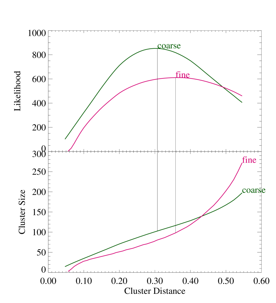
Figure 3: Coarse and Fine Filters. Plots of the of likelihood and cluster size (${\Lambda}$) as a function of distance as computed from the coarse and fine matched filters. The input cluster has a true distance of 0.35 (4.5 billion light years) and size of ${\Lambda}=100$. The coarse likelihood peaks at a distance of 0.31 and estimates the size to be ${\Lambda}=102$. The fine likelihood peaks at a distance of 0.35 and a estimates the size to be ${\Lambda}=98$. In general, the fine likelihood provides better distance and size estimates but at approximately 10 times the computational cost.

Both the coarse and fine likelihood functions are able to exploit the specifics of the model to significantly reduce the number of test locations that need to be evaluated. The coarse likelihood function requires about 10 times less work to evaluate than the fine likelihood. Unfortunately, the underlying assumptions used in the derivation of the coarse likelihood function are not as accurate as those used to derive the fine likelihood. Thus, while the coarse likelihood is faster, the fine likelihood is more accurate (see Figure 3). The AMF addresses this issue by using both likelihood functions in a two stage approach. First, the coarse likelihood function is applied and then the fine likelihood function is used on the peaks found in the coarse map.

Using both filters sequentially not only produces the best estimate of the cluster locations, it has the added benefit of providing two quasi-independent sets of values for each cluster. This provides a helpful consistency check because the coarse and fine filter react differently at the detection limit. The coarse likelihood tends to assign weak detections to small nearby clusters, while the fine likelihood makes these detections large, far away clusters. Thus, if both likelihoods peak at similar size and distance estimates, then the detections are probably real, but if the two likelihoods peak at dramatically different values than the cluster is probably a false detection.

3 Implementation

The likelihood functions derived in the previous section represent the core of the AMF cluster detection scheme. Both likelihood functions begin with picking a grid of test locations. The most straightforward method is to use a regularly spaced grid over $\Omega_{\Theta}$. Recall that each point in $\Theta$ consists of an angular position, a distance and a cluster size and that each point in $X$ consists of an angular position and a brightness. As shown in the previous section, the size can be determined without searching, and a regular grid in distance will work reasonably well provided the steps are sufficiently small (see Figure 3). A regular grid in angle has the difficulty of making the grid too big in dense regions and too fine in sparse regions (i.e., it is unnecessary to search for clusters where there is no data). A more optimal set of test locations is to use the angular positions of the data ${\bf x}_{i}$, which“naturally” provides an adpative resolution.

3.1 Peak Finding

Finding peaks in a 3D regularly gridded map is straightforward. Finding the peaks in the irregularly gridded map is more difficult. There are several possible approaches. We present a simple method which is sufficient for selecting individual clusters. More sophisticated methods will be necessary in order to find small clusters that are close to large clusters.

As a first step we eliminate all low likelihood points ${\cal L}_{\rm coarse}^{i}<{\cal L}_{\rm cut}$, where ${\cal L}_{\rm cut}$ is the nominal detection limit, which is independent of richness or redshift. ${\cal L}_{\rm cut}$ can be estimated from the distribution of the ${\cal L}_{\rm coarse}^{i}$ values. Step two consists of finding the largest value of ${\cal L}_{\rm coarse}^{i}$, which is by definition the first and largest cluster ${\bf\theta}_{1}$. The third step is to eliminate all test points that are within a certain radius of the cluster. Repeating steps two and three until there are no points left results in a complete cluster list $\Theta$. A different scheme would be to connect the irregularly gridded points in a Voronoi tessellation [Ramella 1998] from which local maxima could be obtained in the same manner as on a grid.

3.2 Software Architecture

Implementation of the AMF cluster selection consists of four steps: (1) reading the database and the model parameter files, (2) computing ${\cal L}_{\rm coarse}$ over the entire database, (3) finding clusters by identifying peaks in the ${\cal L}_{\rm coarse}$ map, and (4) evaluating ${\cal L}_{\rm fine}$ and obtaining a more precise determination of each cluster’s size and distance.

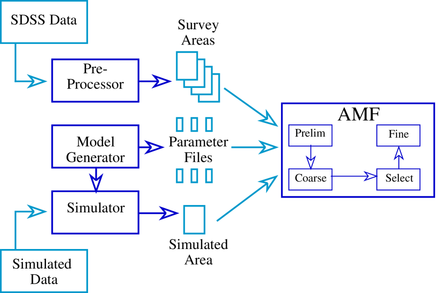
Figure 4: Software Pipeline. Schematic of the AMF software processing pipeline. The processing can accept either real or simulated data. The data is broken up into survey areas and fed into the AMF. The AMF does preliminary data checking followed by the coarse filter. The results of the coarse filter are used to select the locations of clusters which are then fed into the fine filter to provide more accurate estimates. The coarse filter is the dominant step in terms of computing cost.

The architecture of this data processing pipeline is shown in Figure 4. The software has been designed so that it can accept both real and simulated data. One of the challenges of the AMF is organizing the software so that it can readily accept new datasets and different parameter files. Critical to adapting to new data is the ability see into the system and observe each step as it takes place. To address these issues the vast majority of the code has been implemented in an interpreted language (IDL from Research Systems, Inc.) which provides many mechanisms for reading in files and for monitoring and visualizing output.

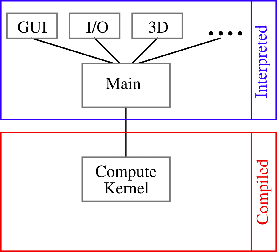
Figure 5: Single CPU Application Architecture. Application architecture before implementation on an Network-Of-Workstations. GUI and other “high level” operations are written in the interpreted layer, which calls the compute kernel (the coarse filter in the AMF application) written in a compiled language.

The computational driver of the application is the evaluation of ${\cal L}_{\rm coarse}$. This function consists of a set of nested for loops which do not lend themselves to the vector notation required to get good performance in an interpreted language. Thus, while the interpreted code is used to set up the calculation, a compiled C routine is called to compute the coarse likelihood function (see Figure 5). In addition to giving the superior compute performance of a compiled language, this layered software approach also provides a mechanism for exploiting parallel computing.

3.3 Parallelization Scheme

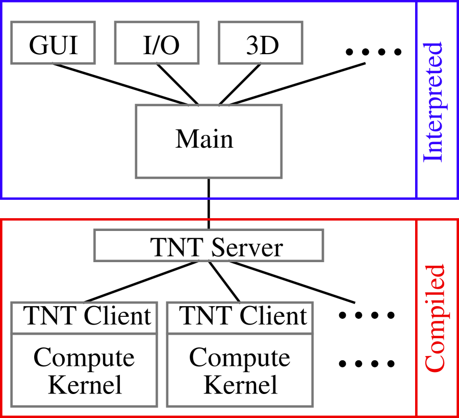
Figure 6: NOW Application Architecture. Application architecture after implementation on an NOW. An additional “TNT” layer has been added to the compute kernel which invokes and manages multiple copies of the compute kernel (coarse filter) on a NOW.

Computing the coarse likelihood map is a highly parallelizable operation. Each test point can be computed independently of the others if all the necessary data is available. There are a variety of ways to take advantage of this scheme. The one chosen here is a client/server approach based on the The Next generation Taskbag (TNT) software library [Kepner et al 2000]. TNT is a client-server based Applications Programming Interface (API) for distributing and managing multiple tasks on a Network-Of-Workstations (NOW). TNT is a C based library which can be used in any compiled program. As such, it is possible to insert the appropriate TNT calls into the compiled layer called by an interpreted language (see Figure 6).

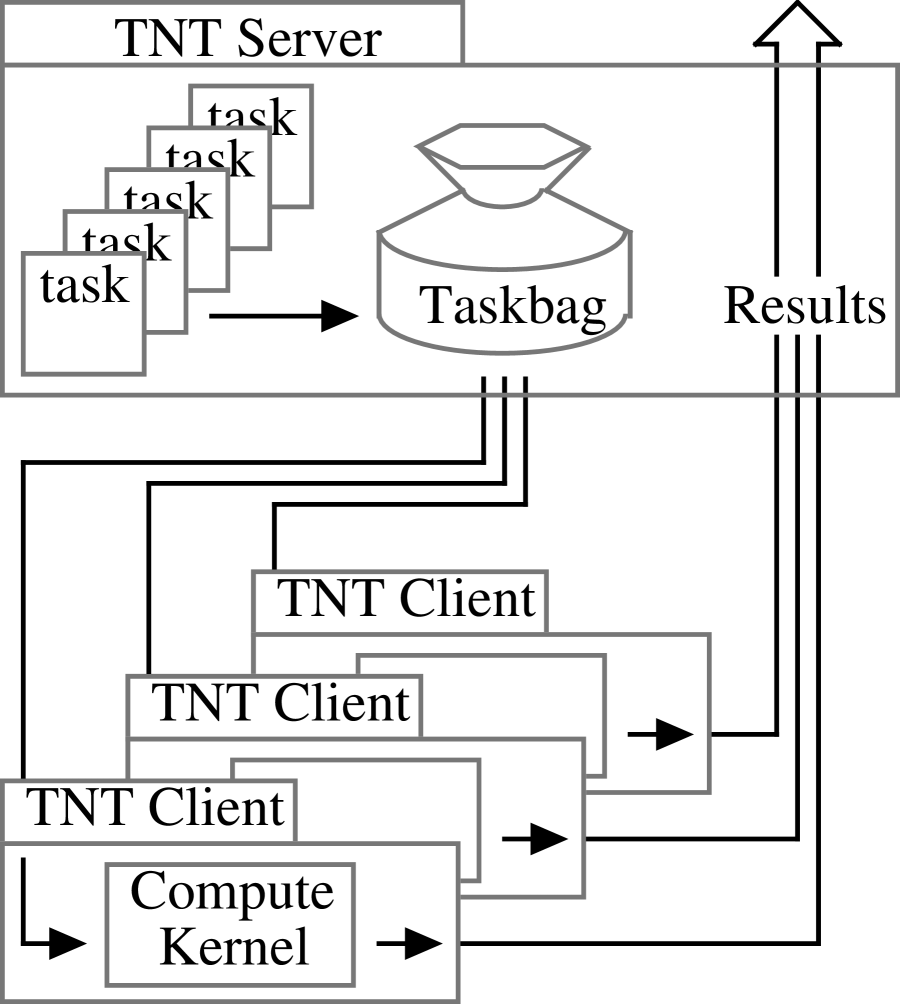
Figure 7: TNT Application A typical TNT application consists of a server with many clients, communicating via TCP/IP. The server: places tasks into Taskbag; listens on a specific port for requests for tasks from clients; dispatches tasks to requesting clients; accepts results from clients; monitors status of clients and re-assigns tasks of dropped clients; when all tasks are completed, returns results back to the main program. The client(s) loop over the Taskbag is until it is empty. On each iteration a client will: send requests for work to server on a specific port; read data sent by server over network; call compute kernel with the data; send results of computation back to server over network. For the AMF, the tasks correspond to sub-sets of the test locations and the compute kernel is the coarse likelihood evaluation.

The operation of a typical TNT application is shown in Figure 7. The server creates a “Taskbag” of work for clients. The clients are then executed remotely on a number of processors. The clients connect with the server and request a task or taskbag (a group of tasks). When they have completed their tasks they return the results back to the server and ask for more tasks.

The TNT library was developed on Linux (RedHat 5.0) and tested on FreeBSD, NetBSD, and Solaris. The entire library is written in C using TCP sockets. A server communicates with the clients using ports, which allows simultaneous servers to be active and listening to different port numbers. A server can call client functions and a client can call server functions. This enables the creation of hierarchies of servers. For example, a “root” server can partition a large taskbag into many sub-taskbags and distribute them to a collection of sub-servers. These sub-servers will then distribute tasks to the clients. This allows for a more efficient distribution of work across the cluster nodes.

For the AMF application, the interpreted language calls a C routine which then sets up a server with tasks to be executed (Figure 7). In this case, each task is a sub-set of all the test points. Clients are then started on other computers (or the same machine if it is multiple processor system). At startup each client receives the database (or a portion of the database) from the server. After receiving the data, each client then asks the server for a task to execute and returns the result.

It is not possible to predict in advance how long a given task is going to take because of the non-linearity of the algorithm and because of heterogeneous capabilities and loads that may exist on the NOW. Fortunately, TNT is inherently load balancing in the sense that when a client finishes a task it requests additional work. If there are no tasks remaining then the client exits and frees up the processor. The processors that run faster will pick up more work and slower processors will pick up less work.

4 Results

The AMF has been extensively tested on simulated data to verify its accuracy and robustness [Kepner et al 1999]. The AMF is currently being applied to detect clusters of galaxies from the Sloan Digital Sky Survey (SDSS) [Kim et al 2000]. The recent parallel implementation of the AMF has significantly increased speed of the application.

4.1 Tests on simulated data

In real data, neither the distances of the galaxies nor the position and sizes of the clusters are known. Tests on simulated data are the only opportunity to check the detection algorithm in a well understood environment. The test data consists of 72 simulated clusters with different sizes and distances placed in a simulated field of randomly distributed galaxies. The data was constructed to be consistent with what is expected from SDSS. The clusters range in size and distance so as to span the full range of expected clusters. The test data covers an area of 10 square degrees (1/1000 of the SDSS) and contains approximately 100,000 points.

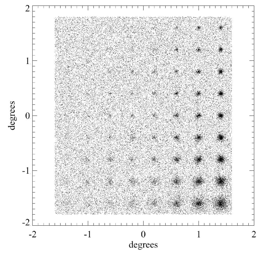
Figure 8: Simulated Data. Angular positions of simulated data containing a uniform field and 72 clusters arranged in an 8 by 9 grid. Each column of clusters are the same size while each row of clusters are at the same distance. From left to right the sizes are $\Lambda=$ 10, 20, 30, 40, 50, 100, 200, and 300. From bottom to top the distances are $z=$ 0.1, 0.15, 0.2, 0.25, 0.3, 0.35, 0.4, 0.45, and 0.5.

To facilitate the subsequent analysis and interpretation of the results, the clusters were placed on an 8 by 9 grid. The cluster centers were separated by 0.4 degrees. The distribution of all the galaxies in angle is shown in Figure 8, where each column of clusters are the same size while each row of clusters are at the same distance. From left to right the sizes are $\Lambda=$ 10, 20, 30, 40, 50, 100, 200, and 300. From bottom to top the distances are $z=$ 0.1, 0.15, 0.2, 0.25, 0.3, 0.35, 0.4, 0.45, and 0.5.

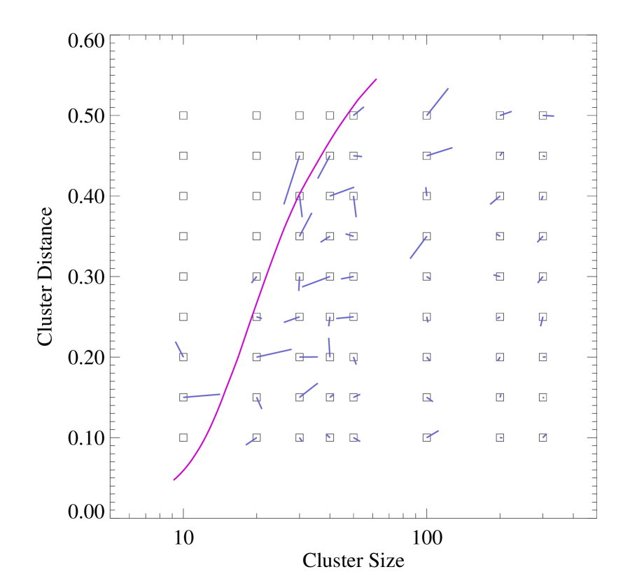
Figure 9: Results from Simulated Data. The size and distance of each of the input clusters (boxes) with the short lines indicating the corresponding values determined from the AMF fine filter. The long curved line indicates the approximate detection limit. All the clusters above the detection limit (i.e. to the right of the line) are found with no false detections. As expected the size and distance estimates are best for the largest and nearest clusters, while clusters near the detection limit have poorer estimates.

The simulated data were run through the AMF and all clusters above the designated 5-$\sigma$ noise limited threshold were detected (with no false detections). The angular positions of all the detected clusters were well within the expected range. The estimated distance and size of each cluster is shown in Figure 9. As expected, the large and/or nearby clusters are detected and measured more accurately than the small, far away clusters. These results indicate that the AMF can detect and unbiasly estimate the location of clusters.

4.2 Tests on SDSS data

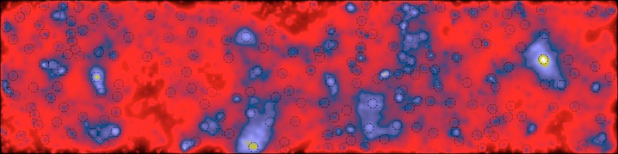
Figure 10: Likelihood Map of Sloan Data. A strip of the Sloan Digital Sky Survey data (courtesy of SDSS Collaboration) was processed through the AMF. This strip covers 30 square degrees and contains nearly 200,000 galaxies. The image shows the projected coarse likelihood map of this strip (red are low values, blue higher, and green is highest). The the dotted circles denote cluster detections.

The Sloan Digital Sky Survey is a multi-decade, multi-institution effort to take a million by million pixel composite image of the night sky in five color bands. Analysis of the image data is expected to yield a database of 200,000,000 galaxies [Szalay et al 1999]. Test data has been taken since 1998 and been used to test all aspects of the SDSS software including the AMF (see Figure 10). The AMF has detected all previously known clusters in the SDSS test data it has looked at. In addition, the AMF performs at a level equal to or better than the other algorithms with which it has been compared. Detailed results and comparison of various cluster finding algorithms are presented elsewhere [Kim et al 2000].

Adapting the AMF to the SDSS was a sizeable effort. Without the layered software approach it would have taken considerably longer as a considerable amount of tuning was required to properly set all the model parameters.

4.3 Scalability results

A parallel implementation of the AMF is crucial for its application to the full SDSS database. Currently, the AMF requires 1-2 hours of CPU time (450 MHz Pentium II) to process a 10 square degree field. On a parallel NOW this can easily be sped up by a factor of 100, which will make processing the entire 10,000 square degree SDSS dataset feasible.

The results of running the parallel implementation on a NOW are shown in Table 1. These data show that the algorithm experiences good speedup on both heterogeneous and homogeneous NOWs. The primary bottlenecks to perfect speedups are the initial sending of data and the granularity of the tasks. The impact of these can be seen in the execution schedules shown in Figures 11-13.

The total computation time consists of the time to do the computation plus the slack time due to the granularity of the tasks

$$T_{\rm comp}\propto\frac{N_{X}}{N_{\rm CPU}}+\frac{N_{X}}{N_{\rm task}}~{},$$ (24)

where $N_{\rm CPU}$ is the number of processors used in the NOW and $N_{\rm task}$ is the number of tasks the job was broken into. The total time spent communicating is the time spent gathering the results plus the time to send the initial data to each processor

$$T_{\rm comm}\propto\frac{N_{X}}{N_{\rm CPU}}+N_{X}N_{\rm CPU}~{}.$$ (25)

To achieve good scalability requires that the computation-to-communication ratio stay high as $N_{\rm CPU}$ increases. In both cases the first term scales well while the second term doesn’t. The second (granularity) term in the computation time is due to the fact that some processors will finish first and there will be no additional tasks for them to complete. This can be alleviated by simply dividing the work up into sufficiently small tasks until this time no longer becomes important.

The second (startup) term in the communication time can be dealt with in several ways. First, the algorithm can be restructured so that each processor gets less data at startup. Second, the communication pattern can be remapped so that the initial data is distributed in multiple steps along a tree. Finally, since the initial data is the same for each processor, it should be possible to use a multicast to allow the data to be distributed everywhere in a single broadcast. Without alleviating this bottleneck the speedup is limited to approximately 100 on a 100 MBit/s class network. If the initial transmit bottleneck can be overcome, it should be possible to see speedups in the 5000 range.

5 Summary and Conclusions

We have presented the Adaptive Matched Filter method for the automatic selection of clusters of galaxies from a galaxy database. The AMF is adaptive in two ways. First, the AMF uses a two step approach that first applies a coarse filter to find the clusters and then a fine filter to provide more precise estimates of the distance and size of each cluster. Second, the AMF uses the location of the data points as a “naturally” adaptive grid to ensure sufficient spatial resolution.

Matched Filter techniques have a firm mathematical basis in statistical signal processing. The AMF uses a hierarchy of two filters (each mathematically correct under its assumptions). Combining these filters allow the AMF to maximize computational performance and accuracy. The AMF also provides two estimates for each cluster which can be compared as an additional check. This is particular effective for these filters because they react differently when given insufficient data.

The AMF relies heavily on models for both the cluster and the background field. This prior information is quite extensive and makes the AMF complex to implement and difficult to adapt to new data sets. To alleviate this coding challenge a hybrid coding approach was used to leverage the ease of use of interpreted languages along with the compute performance of compiled languages. In this way the complex task of testing model inputs and observing their effect through the data processing pipeline can be done quickly without sacrificing the compute efficiency necessary to complete the application in a timely manner.

A further benefit of the hybrid approach is that it makes available to the compiled code a wide variety of parallel software libraries and tools. A parallel implementation is critical to the application because matched filter techniques work by testing every possible location in the cluster space for the presence of a cluster. This is a compute intensive operation, but also provides a high degree of parallelism. The parallelization scheme used for the AMF application is a client/server approach which is a very effective on Network-Of-Workstations. The TNT client/server software used is lightweight and efficient, and provides a naturally load balancing and fault tolerant framework.

The AMF has been extensively tested on simulated data. These results indicate that it robustly and accurately detects clusters and estimates their positions while having few false positives. The AMF is now being applied to the first results of the Sloan Digital Sky Survey [Kim et al 2000]. These tests have shown that the AMF detects all previously known clusters in this data and performs at or above other cluster finding methods. The AMF hybrid application architecture has proven effective in supporting the implementation of new datasets. The TNT based client/server parallelization scheme has also demonstrated significant speedups which will make it feasible for this application to address to the entire SDSS when it becomes available.

$N_{\rm CPU}$	$N_{\rm CPU}$ (eff)	$N_{\rm task}$	Total Time	Speedup	Efficiency
1	1.0	1	5451	-	-
13	10.5	50	700	7.8	74%
13	10.5	200	650	8.4	80%
32	32.0	200	200	27.3	85%

Table 1: AMF Execution Times. Execution times in seconds for various numbers of processors and various numbers of tasks. $N_{\rm CPU}$ is the number of processors used. $N_{\rm CPU}$ (eff) is the number of processors weighted by their clock speed. $N_{\rm task}$ is how many sub-tasks the problem was broken into. The increased parallel efficiency between rows two and three is due to the use of more tasks which results in less slack time due to the task granularity. The increased parallel efficiency between rows three and four is due to the use of a NOW with a higher performing interconnect which reduces the time it takes to initially transmit the data.

Figure 11: Heterogeneous NOW (50 Tasks). Task schedule for the coarse filter running on a heterogeneous NOW consisting of seven single processor and two quad processor workstations. The number in each box shows how many tasks each processor has completed. Task 0 is the initial transmittal of the data. This calculation achieves a speedup of 7.8 out of 10.5 (74%). The barriers to full speedup are the initial transmission and the slack time at the end due the task granularity.

Figure 12: Heterogeneous NOW (200 Tasks). Same as Figure 11 except that the work has been broken up into 200 tasks which reduces the slack time at the end of the calculation resulting in a speedup of 8.4 out of 10.5 (80%).

Figure 13: Homogeneous NOW (200 Tasks). Same as Figure 12 but run on sixteen identical dual processor workstations with a higher performance network. The better network reduces the initial transmit time (Task 0) and results in a speedup of 27.3 out of 32 (85%).

Biographies

Jeremy Kepner received his B.A. in Astrophysics from Pomona College (Claremont, CA). He obtained his Ph.D. focused on Computational Science from the Dept. of Astrophysics at Princeton University in 1998, after which he joined MIT Lincoln Lab. His research has addressed the development of parallel algorithms and tools and the application of massively parallel computing to a variety of data intensive problems. E-mail:jvkepner@astro.princeton.edu or kepner@ll.mit.edu

Rita Seung Jung Kim Rita S.J. Kim is completing her Ph.D. at Princeton University in Astrophysical Sciences. She received her B.S. in Astronomy at Seoul National University (Seoul, Korea), and spent one year in Paris at the Institut d’Astrophysique de Paris. Her thesis work concentrates on the properties of cluster galaxies, and has also worked on statistical modeling of the large scale structure of the Universe. E-mail:rita@astro.princeton.edu

References

- [Abell (1958)] Abell, G. 1958, Astrophysical Journal Supplement, 3, 211
- [Abell, Corwin & Olowin 1989] Abell, G., Corwin, H. & Olowin, R. 1989, Astrophysical Journal Supplement, 70, 1
- [Bahcall 1988] Bahcall, N. 1988, ARA&A, 26, 631
- [Bramel et al 2000] D. A. Bramel, R. C. Nichol, A. C. Pope to appear in the Astrophysical Journal
- [Colley et al 1996] Colley, W.N., Tyson, J.A. & Turner, E.L., 1996, Astrophysical Journal, 461, L83
- [Dalton et al 1994] Dalton, G., Efstathiou, G., Maddox, S. & Sutherland, W. 1994, Monthly Notices of the Royal Astronomical Society, 269, 15
- [Djorgovski et al 1997] Djorgoski, S. et al 1997, to appear in Applications of Digital Image Processing XX, ed. A.Tescher, Proc. S.P.I.E. 3164
- [Dasarathy 1999] B. Dasarathy, 1999, Data Mining and Knowledge Discovery: Theory, Tools and Technology, SPIE Volume 3696
- [Fan & Pando 1997] Li-Zhi Fang & Jesus Pando, Proceedings of the 5th Erice Chalonge School on Astrofundamental Physics, N. Sánchez and A. Zichichi eds., World Scientfic, 1997
- [Fadda et al 1997] Fadda, D., Slezak, E. & Bijaoui, A., 1997, A&A, 127, 335
- [Fayyad et al 1996] U. Fayyad, G. Piatetsky-Shapiro, P. Smyth, and R. Uthurasamy, 1996, Advances in Knowledge Discovery and Data Mining, MIT Press
- [Gal et al 1999] R. R. Gal, R. R. DeCarvalho, S. C. Odewahn, S. G. Djorgovski, V. E. Margoniner, 1999 to appear in Astronomical Journal
- [Kawasaki et al 1997] Kawaski, W., Shimasaku, K., Doi, M. & Okamura, S. 1997 astro-ph/9705112, accepted A&AS
- [Kepner et al 1999] J. Kepner, X. Fan, N. Bahcall, J. Gunn, R. Lupton & G. Xu, 1999 Astrophysical Journal 517, 78
- [Kepner et al 2000] J. Kepner, M. Gokhale, R. Minnich, A. Marks & J. DeGood, 2000 to appear in Cluster Computing
- [Kim et al 2000] Kim et al and the SDSS Collaboration, 2000 Bulletin of the American Astronomical Society, 195, #30.03
- [Lumsden et al 1992] Lumsden, S., Nichol, R., Collins, C. & Guzzo, L. 1992, Monthly Notices of the Royal Astronomical Society, 258, 1
- [Postman et al 1996] Postman, M. et al 1996, Astronomical Journal, 111, 615
- [Ramella 1998] Ramella, M., Nonino, M., Boschlin, W., & Fadda, D. 1998 astro-ph/9810124
- [Szalay et al 1999] Alexander S. Szalay, Peter Kunszt, Anirudha Thakar, Jim Gray, Don Slutz ADASS ’99 conference