Starburst in the Ultra-luminous Galaxy Arp 220 - Constraints from Observations of Radio Recombination Lines and Continuum

Abstract

We present observations of radio recombination lines (RRL) from the starburst galaxy Arp 220 at 8.1 GHz (H92$\alpha$) and 1.4 GHz (H167$\alpha$ and H165$\alpha$) and at 84 GHz (H42$\alpha$), 96 GHz (H40$\alpha$) and 207 GHz (H31$\alpha$) using the Very Large Array and the IRAM 30 m telescope, respectively. RRLs were detected at all the frequencies except at 1.4 GHz where a sensitive upper limit was obtained. We also present continuum flux measurements at these frequencies as well as at 327 MHz made with the VLA. The continuum spectrum, which has a spectral index $\alpha\sim-0.6$ ($S_{\nu}\propto\nu^{\alpha}$) between 5 and 10 GHz, shows a break near 1.5 GHz, a prominent turnover below 500 MHz and a flatter spectral index above 50 GHz.

We show that a model with three components of ionized gas with different densities and area covering factors can consistently explain both RRL and continuum data. The total mass of ionized gas in the three components is $3.2\times 10^{7}$ $M_{\odot}$ requiring $3\times 10^{5}$ O5 stars with a total Lyman continuum (Lyc) production rate N_Lyc $\sim 1.3\times 10^{55}$ photons s^-1. The ratios of the expected to observed Br$\alpha$ and Br$\gamma$ fluxes implies a dust extinction $A_{V}\sim 45$ magnitudes. The derived Lyc photon production rate implies a continuous star formation rate (SFR) averaged over the life time of OB stars of $\sim$ 240 $M_{\odot}$ $yr^{-1}$. The Lyc photon production rate of $\sim$ 3% associated with the high density HII regions implies similar SFR at recent epochs ($t<10^{5}$ yrs). An alternative model of high density gas, which cannot be excluded on the basis of the available data, predicts ten times higher SFR at recent epochs. If confirmed, this model implies that star formation in Arp 220 consists of multiple starbursts of very high SFR (few $\times 10^{3}$ $M_{\odot}$ yr^-1) and short durations ($\sim 10^{5}$ yrs).

The similarity of IR-excess, $L_{IR}/L_{Ly\alpha}\sim 24$, in Arp 220 to values observed in starburst galaxies shows that most of the high luminosity of Arp 220 is due to the on-going starburst, rather than produced by a hidden AGN. A comparison of the IR-excesses in Arp 220, the Galaxy and M33 indicates that the starburst in Arp 220 has an IMF which is similar to that in normal galaxies and has a duration longer than $10^{7}$ yrs. If there was no infall of gas during this period, then the star formation efficiency (SFE) in Arp 220 is $\sim$50%. The high SFR and SFE in Arp 220 is consistent with their known dependences on mass and density of gas in star forming regions of normal galaxies.

email: anantha@rri.ernet.in, fviallef@maat.obspm.fr, niruj@rri.ernet.in

mgoss@aoc.nrao.edu, jzhao@cfa.harvard.edu

Short title: Ionized Gas in Arp 220

1 Introduction

Arp 220 is the nearest ($d$ = 73 Mpc for $H_{0}$ = 75 km s^-1Mpc^-1) example of an ultra-luminous infrared galaxy (ULIRG). ULIRGs are a class of galaxies with enormous infrared luminosities of $L_{IR}\geq 10^{12}L_{\odot}$, believed to have formed through mergers of two gas-rich galaxies (Sanders et al 1988). What powers the high luminosity of ULIRGs is not well understood, although there is considerable evidence that intense starburst which may be triggered by the merger process may play a dominant role (Sanders and Mirabel 1996, Gënzel et al 1998). There is also evidence in many ULIRGs for a dust-enshrouded AGN which could contribute significantly to or in some cases dominate the observed high luminosity (Gënzel et al 1998). In the case of Arp 220, there is clear evidence for a merger in the form of extended tidal tails observed in the optical band (Arp 1966) and the presence of a double nucleus in the radio and NIR bands with a separation of $\sim 1^{\prime\prime}$ (370 pc)(Norris 1985, Graham et al 1990). Prodigious amounts of molecular gas ($M_{H_{2}}\sim 10^{10}M_{\odot}$; Scoville, Yun & Bryant 1997, Downes & Solomon 1998) are present in the central few hundred parsecs. Detection of CS emission (Solomon, Radford & Downes 1990) indicates that the molecular densities may be high ($n_{H_{2}}\sim 10^{5}$ cm^-3). Recent high resolution observations reveal that the two nuclei in Arp 220 consists of a number of compact radio sources - possibly luminous radio supernovae (Smith et al 1998) - and a number of luminous star clusters in the near IR (Scoville et al 1998). High resolution observations of OH megamasers (Lonsdale et al 1998) reveal multiple maser spots with complex spatial structure. These observations have led to the suggestion that the nucleus of Arp 220 is dominated by an intense, compact starburst phenomena rather than the presence of a hidden AGN (Smith et al 1998, Downes & Solomon 1998). The presence of AGNs in the two nuclei is, however, not ruled out since large velocity gradients, $\sim 500$ km s^-1 over $\sim 1^{\prime\prime}$ at different position angles across each nuclei (Sakamoto et al 1999) have been observed, indicating high mass concentrations at the location of both nuclei. Obscuration due to dust in the nuclear region of Arp 220 is extremely high. Ratios of fine structure lines observed with the ISO satellite (Lutz et al 1996, Gënzel et al 1998) indicate a lower limit of $A_{V}\sim$ 45 mag. This high extinction seriously hampers measurements even at IR wavelengths (see also Scoville et al 1998).

Radio recombination lines (RRLs) do not suffer from dust obscuration and thus may potentially provide a powerful method of studying the kinematics, spatial structure and physical properties of ionized gas in the nuclear region of galaxies. RRLs have been detected, to date, in about 15 Galaxies (Shaver, Churchwell and Rots 1977, Seaquist and Bell 1977, Puxley et al 1991, Anantharamaiah et al 1993, Zhao et al 1996, Phookun, Anantharamaiah and Goss, 1998). Arp 220 is the most distant among the galaxies that are detected in recombination lines (Zhao et al 1996). The detection of an RRL in Arp 220 (Zhao et al 1996) opens up the possibility of studying the ionized gas in the nuclear region. Zhao et al (1996) presented VLA observations of the H92$\alpha$ line ($\nu_{rest}$ =8.309 GHz) with an angular resolution of $\sim 4^{\prime\prime}$ and a velocity coverage of $\sim 900$ km s^-1. This paper presents new H92$\alpha$ VLA observations with an angular resolution of $\sim 1^{\prime\prime}$ and a velocity coverage of $\sim 1700$ km s^-1. We also present observations of millimeter wavelength RRLs H42$\alpha$ ($\nu_{rest}$ =85.688 GHz), H40$\alpha$($\nu_{rest}$ = 99.022 GHz) and H31$\alpha$ ($\nu_{rest}$ = 210.501 GHz) made using the IRAM 30 m radio telescope in Pico Veleta, Spain. Additionally, we report a sensitive upper limit to lower frequency RRLs H167$\alpha$ ($\nu_{rest}$ = 1.40 GHz) and H165$\alpha$($\nu_{rest}$ = 1.45 GHz ) obtained using the VLA. These observations together with the observed continuum spectrum are used to constrain the physical properties and the amount of ionized gas in the nuclear region of Arp 220. Since the Lyman continuum photons which ionize the gas are generated by young O and B stars with a finite life time, the derived properties of the ionized gas are used to constrain the properties of the starburst in Arp 220.

The larger velocity coverage used for the present H92$\alpha$ observations showed that the previous observation with half the bandwidth (Zhao et al 1996) had underestimated both the width and the strength of the H92$\alpha$ line. The integrated line intensity is found to be more than a factor of two larger than reported earlier and thus the deduced number of Lyman continuum photons that are required to maintain the ionization is also larger. The millimeter wavelength lines are found to be much stronger than expected based on models for the H92$\alpha$ line. The observed strength of the millimeter wavelength RRLs indicate the presence of a higher density ($n_{e}>10^{5}$ cm^-3) ionized gas component and leads to information about star formation rates at recent epochs ($t<10^{5}$ yrs). The upper limits to the lower frequency lines provide significant constraints on the amount of low density ($n_{e}<10^{3}$ cm^-3) ionized gas in the nuclear region of Arp 220. A comparison of the predictions (based on RRLs) of the strengths of NIR recombination lines (e.g. Br$\alpha$ and Br$\gamma~{}$lines) with observations (e.g. Goldadder et al 1995, Sturm et al 1996) leads to a revised estimate of the dust extinction.

This paper is organized as follows. In Section 2, observations with the the VLA and the IRAM 30 m telescope are described and the results are presented. Section 3 summarizes the available radio continuum measurements of Arp 220 in the frequency range 150 MHz to 230 GHz including new measurements at 327 MHz, 1.4 GHz, 8.3 GHz, 99 GHz and 206 GHz. In Section 3, we discuss the various possible models to explain the observed RRLs and continuum in Arp 220 and arrive at a three-component model, consistent with the observations. Section 4 discusses the implications of the three-component model to several aspects of the starburst in Arp 220. We attempt to answer the question of whether the deduced star formation rates in Arp 220 can power the observed high luminosity without invoking the presence of an obscured active nucleus. The paper is summarized in Section 5.

2 Observations, Data Reduction and Results

2.1 VLA observations and Results

2.1.1 H92$\alpha$ line

Observations of the H92$\alpha$ line ($\nu_{rest}$ = 8309.38 MHz) were made in Aug 1998 in the B configuration of the VLA. The parameters of the observations are given in Table 1. Phase, amplitude and frequency response of the antennas were corrected using observations of the calibrator source 1600+335 ($S_{3.5cm}\sim$ 2 Jy) every 30 minutes. Standard procedures in AIPS were used for generating the continuum image and the line cube. A self-calibration in both amplitude and phase was performed on the continuum channel and the solutions were applied to the spectral line data. For subtracting the continuum, two channels, one on each end (channels 2 and 14), were used in the procedure UVLIN (Cornwel, Uson and Haddad 1992). During off-line data processing, it became necessary to apply hanning smoothing which resulted in a spectral resolution of 6.25 MHz (i.e. 230 km/s) with two spectral points per resolution element. The synthesized beam with natural weighting of the visibility function was $1.1^{\prime\prime}\times 0.9^{\prime\prime}$, PA = 74^∘.

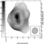
Figure 1: Continuum image of Arp 220 at 8.1 GHz (contours), made using the VLA, with H92$\alpha$ integrated line emission (moment 0) superposed (grey scale). The beam shown at the bottom left corner is $1.1^{\prime\prime}\times 0.9^{\prime\prime}$, PA = 74^∘. The peak continuum brightness is 82 mJy beam^-1. The first contour level is 150 $\mu$Jy beam^-1 and the contour levels progress geometrically by a factor of 1.4. Grey scale for the integrated line intensity covers the range 2 – 120 Jy beam^-1 m s^-1.

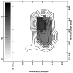
Figure 2: Integrated H92$\alpha$ line emission (moment 0) from Arp 220 in contours with velocity dispersion (moment 2) superposed in grey scale. Beam is same as in Fig 1. Contour peak flux is 130 Jy beam^-1 m s^-1. Contour levels are 1, 2, 3 … percent of the peak. The grey scale covers the range 50 – 180 km s^-1.

The continuum image of Arp220 is shown in Fig 1 as contours with the image of the velocity-integrated H92$\alpha$ line (moment 0) superposed in grey scale. The two radio nuclei of Arp 220 (Norris et al 1988) which are separated by about $1^{\prime\prime}$ are barely resolved. Fig 1 shows that the recombination line emission is detected from both nuclei. The peak of the line emission is slightly offset to the north with respect to the continuum peak. The position angle of the elongated line emission is tilted with respect to the line joining the two continuum peaks by $\sim+7^{\circ}$. Fig 2 shows a contour image of the velocity-integrated line emission (moment 0) with velocity dispersion (moment2) superposed in grey scale. The recombination line is stronger and wider near the western source and there appears to be a weak extension of the ionized gas towards the north-east.

Fig 3 shows the integrated H92$\alpha$ line profile (top frame) along with line profiles near the eastern and western continuum peaks. The line profile is wider on the western peak. The parameters of the integrated line profile are given in Table 2. The spatially-integrated H92$\alpha$ line has a peak flux density of 0.6 mJy/beam and a FWHM of 363 km s^-1. Both these values are larger than the values reported by Zhao et al (1996). The integrated line flux is 8$\times 10^{-23}$ W m^-2 which is a factor of 2.3 larger than the values reported by Zhao et al (1996). The integrated flux was underestimated by Zhao et al (1996) since a narrower bandwidth was used in their observation, thereby missing a portion of the line.

Because of the coarse velocity resolution (230 km s^-1) of the H92$\alpha$ data, detailed information about the kinematics is limited. Fig 4a shows a position-velocity diagram along the line joining the two continuum peaks (P.A. = 98^∘). The velocity range is wider near the western peak compared to the eastern peak. After correcting for the instrumental resolution, the full velocity range over the western peak is about 700 km s^-1. On the eastern peak the velocity range is 440 km s^-1. The FWHMs on the western and the eastern peaks are 500 km s^-1and 340 km s^-1respectively. Fig 4b shows a position-velocity diagram along the line perpendicular to the line joining the two peaks. The full velocity range of emission in Fig 4b is about 770 km s^-1with a FWHM of 430 km s^-1. No velocity gradients are visible in Figs 4a and 4b.

2.1.2 H167$\alpha$ and H165$\alpha$ Lines

The H167$\alpha$ ($\nu_{obs}$ = 1399.37 MHz) and the H165$\alpha$ ($\nu_{obs}$ = 1450.72 MHz) lines were observed simultaneously over a 7 hour period in March 1998 in the A configuration of the VLA. Observational details are summarized in Table 1. Data were processed using standard procedures in AIPS. With natural weighting of the visibilities, the beam size is $1.8^{\prime\prime}\times 1.6^{\prime\prime}$. The peak continuum flux density was 215 mJy/beam and the integrated flux density is 312$\pm$3 mJy. After hanning smoothing, the resolution of each spectral channel was 390 kHz ($\sim 84$ km s^-1) and the rms noise was $\sim 130~{}\mu$Jy/beam. Neither line was detected. For a line width of 350 km s^-1, we obtain a $3\sigma$ upper limit to the line strength of 0.25 mJy. The parameters are listed in Table 2. As shown in the next section, the upper limit to the RRLs near 1.4 GHz provide significant constraints on the density of ionized gas in Arp 220.

2.2 IRAM-30 m Observations and Results

Observations with the IRAM-30 m telescope in Pico Veleta, Spain were carried out on April 19, 1996. The pointing of the telescope was adjusted from time to time; the rms pointing error was $\sim 3^{\prime\prime}$. Three receivers were used simultaneously. A 1.2 mm receiver connected to a 512 MHz filter bank spectrometer was used to observe the H31$\alpha$ line ($\nu_{rest}$ = 210.5018 GHz). The other two receivers were used to observe the H40$\alpha$ ($\nu_{rest}$ = 99.0229 GHz) and the H42$\alpha$ ($\nu_{rest}$ = 85.6884 GHz) lines in the 3 mm band. The two 3 mm lines were observed using two subsets of the autocorrelation spectrometer, each with 409 channels. Instrumental parameters are summarized in Table 3. In the 1.2 mm band, the system temperature ranged between 260 K and 285 K and in the 3 mm band, the system temperatures were between 180 K and 200 K. The wobbler was used to remove the sky emission and to determine the instrumental frequency response. Spectra were recorded every 30 seconds.

The data from the IRAM-30 m telescope were reduced using a special program written by one of us (FV) to reduce single-dish spectral data in the Groningen Image Processing System (GIPSY) environment (van der Hulst et al 1992). In this new program, a baseline subtracted final spectrum as well as a continuum level are simultaneously determined from the data base which consists of a series of spectra sampled every 30 s. The temporal information is used to perform statistics on the data to measure the rms noise as a function of integration time and frequency resolution. These statistics also provide the uncertainties associated with the fitted baselines. These measured uncertainties are used in the determination of error bars in the line and continuum flux densities. In addition, the program also determines a statistical rms noise level for each spectral channel separately, which helps in judging the reality or otherwise of a spectral feature. The details of this procedure are described by Viallefond (2000, in preparation).

The final spectra obtained with the IRAM-30 m data are shown in Fig 5 and the parameters are listed in Table 4. The quoted error bars are the quadrature sums of the system noise and baseline uncertainties. To obtain the H42$\alpha$ spectrum shown in the bottom panel of Fig 5, linear baselines were fitted over the velocity ranges 4600-5050 km s^-1and 5800-6200 km s^-1. The spectrum has been smoothed to a resolution of 30 MHz and re-sampled to obtain 17 independent frequency channels out of the original 409 channels. The H42$\alpha$ recombination line extends from 5050 km s^-1to 5800 km s^-1. The emission feature at the higher velocity end of the spectrum (i.e $v>$ 6200 km s^-1) is probably the rotational line of the molecule C₃H₂ ($\nu_{rest}$ = 85.339 GHz). The continuum level is poorly determined from this data set and thus only a $3\sigma$ upper limit to the continuum flux density is listed in Table 4.

The H40$\alpha$ spectrum shown in the middle panel of Fig 5 was determined by fitting linear baselines to channels outside the velocity range 4950-5850 km s^-1. The spectrum has been smoothed to a resolution of 30 MHz and re-sampled at 17 independent frequency points. The dashed lines in Fig 5 shows the rms noise across the spectrum determined as described in Viallefond (2000, in preparation). The H40$\alpha$ line emission is quite similar to the H42$\alpha$ emission in Fig 5. The consistency between the two lines confirms the reality of the detections. This data set also provided a measurement of the continuum flux density near 3 mm which is listed in Table 4

The observations of the H31$\alpha$ line near 202.7 GHz have a serious limitation. The 512 MHz ($\sim$750 km s^-1) bandwidth used for the observations was too small to cover the entire extent of the line (FWZI $>$ 800 km s^-1). To determine the continuum emission and the spectral baseline level, we used the few channels at one end of the spectrum where no line emission was expected. Although the resulting spectrum, shown as a solid line in the top panel of Fig 5, covers only a part of the line emission, it is consistent in shape with the other recombination lines in Fig 5. The statistical significance of the detection of the H31$\alpha$ line is $>10\sigma$ near the peak. Table 2 lists the ratios of the strengths of various recombination lines integrated over the partial velocity range 5220-5755 km s^-1over which the H31$\alpha$ line has been observed. The strength of the H31$\alpha$ line over the full extent of the line is estimated based on these ratios.

The millimeter wavelength recombination lines (H42$\alpha$, H40$\alpha$ and H31$\alpha$) detected with the IRAM-30 m telescope are much stronger than the centimeter wavelength line (H92$\alpha$) detected with the VLA. While the peak line strength at $\lambda$ = 3.5 cm (H92$\alpha$) is 0.6 mJy, the corresponding lines at $\lambda$ = 3 mm (H40$\alpha$) and 1.2 mm (H31$\alpha$) are an order of magnitude more intense: 15 mJy and 80 mJy, respectively. An increase in the recombination line strength at millimeter wavelengths was expected from high density models discussed by Anantharamaiah et al (1993) and Zhao et al (1996). However, the observed increase in the line strength is much larger than expected on the basis of the models for the H92$\alpha$ line. The mm RRLs H40$\alpha$ and H42$\alpha$ also appear to be broader than the cm RRL H92$\alpha$ line. The width of the mm RRLs are comparable to that of CO lines (Downes and Solomon 1998).

3 Radio Continuum Spectrum of Arp 220

As a byproduct of the RRL measurements, continuum flux densities are obtained at 1.4, 8.2, 97.2 and 206.7 GHz. The measured flux densities are listed in Table 5 along with published values at other frequencies. The continuum flux density measurements around 1.5 mm are consistent with the determination by Downes and Solomon (1998), but the value near 3 mm is higher than that reported by the same authors. The increase in the flux density above 200 GHz is due to contribution by thermal dust emission.

In addition, we observed Arp 220 near 0.325 GHz in August 99 using the A-configuration of the VLA using 3C286 as the flux calibrator. The angular resolution was $\sim 6.5^{\prime\prime}$. Arp 220 is unresolved with this beam. The integrated flux density of Arp 220 is 380$\pm$15 mJy. A flux density measurement at an even lower frequency of 0.15 GHz has been reported by Sopp and Alexander (1991), which is also included in Table 5.

The continuum spectrum in the frequency range 0.1 to 100 GHz is plotted in Fig 6. The continuum spectrum is non-thermal in the frequency range 3 to 30 GHz with a spectral index $\alpha\sim-0.6$ (where $S_{\nu}\propto\nu^{\alpha}$). The spectrum changes both below and above this frequency range. A break in the spectrum is observed around 2 GHz with a change in the spectral index to $\sim-0.1$ between 1.6 GHz and 0.325 GHz. A further change in spectrum occurs below 300 MHz. The spectral index changes to $\sim+0.5$ and between 0.325 GHz and 0.15 GHz. These changes in the spectrum at lower frequencies are complex and cannot be explained by a simple free-free absorbing thermal screen or thermal gas mixed with the non-thermal component (e.g. Sopp & Alexander 1991). At the higher frequencies the change in the spectrum is gradual. The spectral index appears to become slightly flatter (i.e. $\alpha>-0.6$) above 22.5 GHz. The solid line in Fig 6 is a fit to the continuum spectrum based on a 3-component ionized gas model (next section) developed to explain the observed recombination lines.

4 Models for RRL and Continuum emission

Models for RRL emission from the nuclear region of external galaxies have been discussed by Puxley et al (1991), Anantharamaiah et al (1993), Zhao et al (1996, 1998) and Phookun et al (1998). The main constraints for these models are the integrated RRL strength at one or more frequencies, the observed radio continuum spectrum and geometrical considerations. Two types of models have been considered: one based on a uniform slab of ionized gas and the other based on a collection of compact HII regions. The observed non-thermal radio continuum spectrum of the nuclear region, with spectral index $\alpha\leq-0.6$ (where $S_{\nu}\propto\nu^{-\alpha}$), imposes strong constraints on the nature of the ionized gas that produces the observed recombination lines from the same region. If the models are constrained by a single RRL measurement and the continuum spectrum, then the derived physical parameters ($T_{e},n_{e},M_{HII}$ etc) are not unique. In a majority of the cases that were considered (Anantharamaiah et al 1993, Zhao et al 1996, Phookun et al 1998), the model with a collection of compact, high density HII regions is favored. The uniform slab models produce an excess of thermal continuum emission at centimeter wavelengths inconsistent with the observed non-thermal spectrum. However, in the case of Arp 220, Zhao et al (1996) were able to fit both types of models; thus further observations at higher and lower frequencies were required to choose between the models. We consider below these models of RRL emission in the light of the new measurements.

4.1 Uniform Slab Model

In the uniform slab model, the parameters are the electron temperature ($T_{e}$), the electron density ($n_{e}$) and the thickness of the slab (l). For a given combination of $T_{e}$ and $n_{e}$, l is adjusted to account for the observed integrated H92$\alpha$ line strength. While calculating the line strength, stimulated emission due to the background non-thermal continuum, as well as internal stimulated emission due to the thermal continuum emission from the ionized gas are taken into account. The relevant expressions for the computation are given by Anantharamaiah et al (1993). The observed total continuum emission at two frequencies, together with the computed thermal emission from the ionized slab, is used to estimate the intrinsic non-thermal emission and its spectral index. Models in which the thermal emission from the slab at 5 GHz exceeds a substantial fraction ($\sim$ 30 – 50%) of the total continuum emission are rejected since the resulting spectral index will not be consistent with the observed non-thermal spectrum. Finally, the expected variation of line and continuum emissions as a function of frequency are computed and compared with the observations.

Fig 7a shows the expected variation of integrated RRL strength as a function of frequency for $T_{e}$= 7500 K and three values of electron density. Fig 7b shows the expected variation of continuum emission for the corresponding models. In these models, the slab of ionized gas is assumed to be in front of the non-thermal source. Results are qualitatively similar if the ionized gas is mixed with the non-thermal gas. The models are normalized to the H92$\alpha$ line and the continuum flux densities at 4.7 and 15 GHz. Fig 7 shows that while the non-thermal continuum spectrum above 2 GHz and the change in the spectrum near 1.6 GHz agree with the models, the flux densities at 0.15 and 0.325 GHz are not explained. In all the models, free-free absorption is prominent below 1.5 GHz. No uniform slab model can be found which both accounts for the H92$\alpha$ line and also produces a turnover in the continuum spectrum at a frequency $<$ 1.5 GHz. Furthermore, all the models that fit the H92$\alpha$ line predict a strength for RRLs near 1.4 GHz line inconsistent with the upper limit. For other values of $T_{e}$ (5000 K and 10000 K), the curves are similar to Figs 7a and 7b. No models with $n_{e}>10^{3}$ cm^-3 could be fitted to the H92$\alpha$ line. The parameters of the models shown in Fig 7 are given in Table 6. In these models, external stimulated emission (i.e. due to the background non-thermal radiation) accounts for more than 75% of the H92$\alpha$ line strength. No uniform slab model, at any density, could be fitted to the higher frequency (H42$\alpha$, H40$\alpha$ and H31a) lines. Since all the uniform slab models are inconsistent with low frequency RRL and continuum data, we consider models with a collection of HII regions.

4.2 Model with a Collection of HII regions

In this model, the observed RRLs are thought to arise in a number of compact, high density HII regions whose total volume filling factor in the nuclear region is small ($<10^{-4}$) (Puxley et al 1991, Anantharamaiah et al 1993). The low volume filling factor ensures that the HII regions, regardless of their continuum opacities, have only a small effect on the propagation of the non-thermal continuum which originates in the nuclear region. Thus, the observed radio continuum spectrum can be non-thermal even below the frequency at which the HII regions themselves become optically thick. The low filling factor also implies that in these models there is little external stimulated emission. Since the HII regions are nearly optically thick at centimeter wavelengths, they produce only a modest amount of thermal continuum emission (typically $<$ 30% of S_obs). The recombination line emission from these regions arises mainly through internal stimulated emission due to the continuum generated within the HII regions. If the density of the HII regions are lower ($n_{e}<10^{3}$ cm^-3) and the area covering factor $f_{c}$ (i.e. the fraction of the area of the non-thermal emitting region that is covered by HII regions) is larger, then external stimulated emission can become dominant at centimeter wavelengths.

For simplicity, all the HII regions are considered to be characterized by the same combination of $T_{e}$, $n_{e}$ and diameter $d_{\scriptstyle HII}$. For a given combination of these parameters, the expected integrated line flux density ($\int S_{l}d_{\nu}$) of a single HII region is calculated using standard expressions (e.g. Anantharamaiah et al 1993). The number of HII regions is then computed by dividing the integrated flux density of one of the observed RRLs (e.g. H92$\alpha$) by the expected strength from a single HII region. Since the volume filling factor of the HII regions is small, the effect of shadowing of one HII region by another is not significant. Constraints from the observed continuum flux densities at various frequencies and from several geometrical aspects, as discussed in Anantharamaiah et al (1993), are applied to restrict the acceptable combinations of $T_{e}$, $n_{e}$ and $d_{\scriptstyle HII}$. Finally, the models are used to compute the expected variation of line and continuum emission with frequency and compared with observations. We show below that separate components of ionized gas are required to explain the centimeter wavelength (H92$\alpha$) and millimeter wavelength RRLs (H42$\alpha$, H40$\alpha$ and H31$\alpha$).

4.2.1 Models based on the H92$\alpha$ line and the Continuum

Fig 8 shows three representative models that fit the observed H92$\alpha$ line. The parameters of the three models are given in Table 7. The nature of the curves for other successful combinations of $T_{e}$, $n_{e}$ and $d_{\scriptstyle HII}$ are similar to one of the three curves shown in Fig 8, although the values of the derived parameters are different. At densities below about 500 cm^-3, the area covering factor of the HII regions is unity. In other words, every line of sight through the line emitting region intersects at least one HII region (N${}_{los}^{\scriptstyle HII}$$>1$ and $f_{c}$ =1 in Table 7), and thus the models at these densities are similar to the uniform slab model discussed above. As seen in the dashed curves in Fig 8, these low-density models are inconsistent with the continuum spectrum below 1 GHz as well as the upper limit to the RRL emission near 1.4 GHz. Lower density models, which were considered possible by Zhao et al (1996) based only on the H92$\alpha$ and higher frequency continuum data, are now ruled out.

At densities above about 5000 cm^-3, the area filling factor of the HII regions is very small ($f_{c}<<$ 1) and thus they do not interfere with the propagation of the non-thermal radiation. The continuum spectrum will be non-thermal even at the lowest frequencies. The dash-dot-dash curve in Fig 8 shows such a model (model C1) with the parameters given in Table 7. In this model, although there are more than $10^{5}$ HII regions, each $\sim$1 pc in diameter and optically thick below $\sim$ 3 GHz, the total continuum emission continues to have a non-thermal spectrum at lower frequencies. Thus these higher density models cannot account for the observed turnover in the continuum spectrum at $\nu<$ 500 MHz. These models are however consistent with the upper limit to the RRL emission near 1.4 GHz.

A continuum spectrum, which is partially consistent with observations at low frequencies is obtained by models with densities in the range $750<n_{e}<1500$ cm^-3. An example is the solid curve in Fig 8 (Model A1) with the parameters as given in Table 7. For this model, the area covering factor $f_{c}=$ 0.7. In other words 30% of the non-thermal radiation propagates unhindered by the HII regions and the remaining 70% is subjected to the free-free absorbing effects of the HII regions. The net continuum spectrum thus develops a break near the frequency at which $\tau_{HII}\sim 1$. At much lower frequencies where 70% of the non-thermal radiation is completely free-free absorbed, the remaining 30% propagates through with its intrinsic non-thermal spectrum as shown in the solid curve in Fig 8. While this model accounts for the break in the spectrum near $\sim$ 2 GHz, it fails to account for the complete turnover in the continuum spectrum below 500 MHz. An additional thermal component with a covering factor close to unity and a turnover frequency near $\sim$ 300 MHz is required to account for the low-frequency spectrum. This component is discussed in Section 4.2.3. Model A1 in Fig 8 is also consistent with the upper limit to the RRL emission near 1.4 GHz.

In the models shown in Fig 8 and Table 7, between 25% to 70% of the line emission arises due to external stimulated emission, i.e. amplification of the background non-thermal radiation at the line frequency due to non-LTE effects. For lower densities, the fraction of external stimulated emission is increased. For $n_{e}\sim 1000$ cm^-3 (favored above), 70% of the H92$\alpha$ line is due to stimulated emission. The other parameter of interest in Table 9 which is related to the line emission mechanism is the non-LTE factor $f_{nlte}$, the ratio of the intrinsic line emission from an HII region if non-LTE effects are included to the line emission expected under pure LTE conditions (i.e. $b_{n}=\beta_{n}=1$). $f_{nlte}$ is in the range 1 to 3 for the models in Table 7. For lower densities, the non-LTE effect on the intrinsic line emission from an HII region are reduced. Thus, in the models with a collection of HII regions, external and internal stimulated emissions vary with density in opposite ways. If the density is increased, internal stimulated emission increases whereas external stimulated emission decreases.

Two important parameters that can be derived from these models are the mass of the ionized gas M_HII and the number of Lyman continuum (Lyc) photons N_Lyc . The latter can be directly related to the formation rate of massive stars if direct absorption of Lyc photons by dust is not significant. Furthermore, predictions can be made for the expected strengths of optical and IR recombination lines, which can then be compared with observed values in order to estimate the extinction. Some derived quantities are listed in Table 7. As seen in this Table, although a range of $n_{e}$, $T_{e}$, and $d_{\scriptstyle HII}$ values fit the H92$\alpha$ data, the derived value of N_Lyc varies by less than a factor of two. For the model labelled A1 in Fig 8, the total mass of ionized gas M_HII = $3\times 10^{7}$ $M_{\odot}$ and the number of Lyman continuum photons N_Lyc = $1.2\times 10^{55}$ s^-1. For models that satisfy all the constraints, the derived parameters M_HII  and N_Lyc  increase if either $T_{e}$ is increased or $d_{\scriptstyle HII}$ is decreased. On the other hand, as the density $n_{e}$ is increased, M_HII  decreases, whereas N_Lyc first increases and then decreases.

None of the models (at any density) that fit the H92$\alpha$ line can account for the observed H42$\alpha$, H40$\alpha$ and H31$\alpha$ lines. Although an increase in line strength towards shorter wavelengths is predicted by all the models (Fig 8), the expected integrated line flux density falls short by almost an order of magnitude, well above any uncertainty in the measurements. The model A1 in Fig 8 can explain the H92$\alpha$ line, the break in the continuum spectrum at 1.5 GHz and is consistent with the upper limit to the H167$\alpha$ line. Additional components of ionized gas are required to explain the millimeter wavelength RRLs and the turnover the continuum spectrum below 500 MHz.

4.2.2 Models based on the H42$\alpha$ line and the Continuum

Since no model that fits the H92$\alpha$ line could account for the observed 3 mm and 1.2 mm lines, separate models, also based on a collection of HII regions, were fitted to the H42$\alpha$ line. Only models with densities above $10^{5}$ cm^-3 are consistent with the mm wavelength RRLs. Three successful models, labelled A2, B2, and C2 are shown in Fig 9 and the parameters of the models are listed in Table 8. As seen in Fig 9, the contribution of this high density component to RRLs at centimeter wavelengths is negligible since the HII regions are optically thick at these frequencies. This high density component is thus detectable only in RRLs at millimeter wavelengths.

In the models summarized in Table 8, the contribution to the line emission from external stimulated emission is negligible ($<0.5\%)$. On the other hand, enhancement of the line due to internal stimulated emission within the HII regions is pronounced and sensitive to the parameters of the HII regions ($n_{e}$, $T_{e}$, and $d_{\scriptstyle HII}$). The factor $f_{nlte}$ range from 30 - 1300 for the models in Table 8. Because of the sensitivity of the expected line strength to parameters of the HII regions, the derived quantities (M_HII and N_Lyc ) can be well constrained by the observed relative strengths of the H40$\alpha$ and H31$\alpha$ lines. Fig 9 indicates that the high density models can also be distinguished by their contribution to the continuum flux density at mm wavelengths.

The Model labelled A2 in Fig 9 (and Table 8) gives a good fit to the observed relative strengths of the H31$\alpha$, H40$\alpha$, and H42$\alpha$ lines. The solid line in Fig 9(b) shows the expected continuum spectrum if only thermal emission from component A2 is added to the non-thermal emission. Because of the low area filling factor ($f_{c}$) of these components, there is no effect on the propagation of the non-thermal radiation, although the HII regions are optically thick below about 40 GHz. Thermal emission from component A2 at 100 GHz is only about 0.6 mJy. In this model, the mass of ionized gas M_HII = $3.6\times 10^{3}$ $M_{\odot}$ which is negligible compared to the mass of component A1, $6\times 10^{7}$ $M_{\odot}$ (Table 7), required to explain the H92$\alpha$ line. The number of Lyman continuum photons N_Lyc for the high density component A2 is $3.5\times 10^{53}$ s^-1, about 3% of that for the lower density component A1 (Table 7).

The parameters of the high density component that fit the mm wavelength RRLs are not unique. The alternative model B2, shown as a dashed line in Fig 9, which is reasonably consistent with the mm RRLs has a factor of ten higher M_HII  and N_Lyc  (see Table 8). This model contributes a higher thermal continuum flux density ($\sim 8$ mJy) at 100 GHz (see Fig 9). A better determination of RRL and continuum flux densities are required to choose between models A2 and B2. As discussed in section 5.4, the high density component provides important information about the star formation rate during recent epochs in Arp 220.

4.2.3 A Combined Model with Three Ionized Components

In this section, we combine the best-fitting models presented in the previous two sections and introduce a third component to account for all the observations. As discussed above, no single-density ionized component is consistent with all the observations. The presence of multiple components of ionized gas is to be expected since it is extremely unlikely that a complex starburst region like Arp 220 could consist of a single density ionized component. To construct a three component model, we first select two models which provide good fits to the H92$\alpha$ and H42$\alpha$ lines. We selected models which are labelled A1 and A2 in Figs 8 and 9, respectively. The parameters of these models are listed in Tables 7 and 8. The sum of the contributions from these two models to the line emission can account for both H92$\alpha$ and H42$\alpha$ and also is consistent with H40$\alpha$ and H31$\alpha$ line and the upper limit to the H167$\alpha$ line. Fig 10 illustrates the line and continuum emission from these two components. These two components together can also account for the continuum spectrum above 1 GHz. In this model, the intrinsic non-thermal emission has a spectral index $\alpha\sim-0.8$. Because of the presence of the thermal components, the spectral index changes to $\sim-0.6$ in the range 2–20 GHz. A break in the spectrum is observed near 2 GHz which can be accounted for by component A1. This component, which has an area covering factor of 0.7, becomes optically thick around 2 GHz and therefore progressively absorbs about 70% of the non-thermal radiation at lower frequencies. Component A2, which becomes optically thin above $\sim 40$ GHz, contributes very little to the continuum emission at any wavelength. Thermal contribution to the continuum emission comes mainly from component A1 and it becomes significant in comparison to the non-thermal component above $\sim 20$ GHz. The thermal and non-thermal emissions contributions are about equal at $\nu\sim$ 50 GHz. Since the thermal component exceeds the non-thermal component above 50 GHz, the continuum spectrum becomes flatter at millimeter wavelengths. In the continuum spectrum shown as a solid line in Fig 10b, thermal dust emission, which may have a significant contribution even at 100 GHz, has not been included. Above 200 GHz, the total continuum is dominated by dust emission (Rigopoulou et al 1996, Downes and Solomon 1998). From the sub-millimeter continuum measurements by Rigopolou et al (1996), we estimate that $\sim$20% of the continuum emission at 3 mm could be contributed by dust.

The observed continuum spectrum below a few hundred MHz is not accounted for by the two thermal components A1 and A2 discussed above. An additional free-free absorbing component with an emission measure of a few times $10^{5}$ pc cm^-6 and an area covering factor $f_{c}\sim 1$ is needed to account for the observed turnover. Furthermore, the flux densities measured at 327 MHz and 150 MHz (Table 5) indicate that the roll off in the spectrum is not steep enough to be accounted for by a foreground thermal screen. On the other hand, if the thermal gas is mixed with the non-thermal emitting gas, then a shallower roll off is expected. It was possible to obtain a good fit to the observed spectrum by adding a thermal component (mixed with the non-thermal gas) with an emission measure EM = $1.3\times 10^{5}$, $n_{e}$= 1000 cm^-3, $T_{e}$= 7500 K and an area covering factor of unity. The line and continuum emission of this component (shown as model D in Fig 10) is very weak and is practically undetectable at any frequency. The only observable aspect of this component is the turnover in the continuum spectrum below a few hundred MHz. The main constraint for this component is its emission measure. Densities lower than about 500 cm^-3 can be ruled out as they are inconsistent with the upper limit to RRLs near 1.4 GHz. For the model shown in Fig 10, $n_{e}$=1000 cm^-3 and $T_{e}$=7500 K which are same as those of component A1.

All the parameters of this ionized component (model D) along with those of components A1 and A2 and the sum of the three components, where appropriate, are given in Table 9. Less than 10% of the ionized mass is in component D and $\sim$ 6% of the Lyman continuum photons arise from this component. Most of the mass (94%) is in component A1, accounting for $\sim 92$% of the total Lyman continuum photons. The mass in the high density component (A2) is negligible ($\sim 0.01$%) and it accounts for about 3% of the Lyman continuum photons.

Although the models given in Table 9 provide good fit to the observed line and continuum data as seen in Fig 10, there are two aspects which are not satisfactory: (1) Component A1, which contains the bulk of the ionized gas at a density around 1000 cm^-3, is barely consistent with the upper limit to the H167$\alpha$ line. In fact, if this model is correct, then the H167$\alpha$ line should be detectable with a factor of 2-3 increase in sensitivity. Although an increase in density of this component will reduce the intensity of the H167$\alpha$ line (e.g. model C1 in Fig 8), the model will then fail to account for the observed break in the continuum spectrum around 1.5 GHz. (2) Model B2 in Fig 9, which is an alternative to A2 also provides a reasonable fit to the observations, but has an order of magnitude higher M_HII and N_Lyc . This model slightly overestimates the continuum flux density near 100 GHz but it provides a good fit to the mm wavelength RRLs. As explained in Section 5.4, there are significant implications to the star formation history of Arp 220 if N_Lyc in the high density component is as high as in component B2. A resolution of the two difficulties mentioned here must await a firm detection or determination of a more sensitive upper limit to the H167$\alpha$ line and a more accurate determination of the line and continuum parameters at millimeter wavelengths. The validity or otherwise of model B2 can be determined if several mm wavelength RRLs and continuum are observed in the frequency range 100 to 300 GHz and a proper separation of continuum emission by dust and ionized gas is performed using the data.

5 Discussion

5.1 Density

As discussed in the previous section, only models with densities $>\sim 10^{3}$ cm^-3 can fit the recombination line data. Lower density models are inconsistent with the upper limit to the recombination line strength near 20 cm. While densities in the range $10^{3}-2.5\times 10^{4}$ cm^-3 fit the H92$\alpha$ line, even higher densities ($n_{e}$$\sim 1-5\times 10^{5}$ cm^-3) are required to account for the millimeter wavelength recombination lines. These results confirm the point made by Zhao et al (1996) that recombination lines at different frequencies act as “density filters”. Thus multi-frequency RRL observations provides an excellent method of determining the various density components in starburst regions.

That a substantial fraction of the gas in the nuclear regions of Arp 220 is at densities $>10^{4}$ cm^-3 is evident from the high ${\rm L_{HCN}/L_{CO}}$ ratio observed by Solomon, Downes and Radford (1992). The total mass of H₂ gas at densities higher than $10^{4}$ cm^-3 is $>10^{9}$ $M_{\odot}$ or more than 25% of the dynamical mass of the two nuclear components (Downes & Solomon 1998). Less than $10^{-4}$ of this gas needs to be in ionized form to account for the high density ionized gas deduced from millimeter wavelength recombination lines. The bulk of the ionized gas ($\sim 3\times 10^{7}$ $M_{\odot}$) which is in component A1 (Table 9) is at a density $\sim 10^{3}$ cm^-3 or higher.

Electron densities inferred from [S III] and [Ne III] IR line ratios observed with the ISO satellite typically yield lower values ($n_{e}\sim 100-300$ cm^-3) (Lutz et al 1996). We suggest that this is a selection effect caused by the insensitivity of the [S III] line ratios to densities outside the range $10^{2}-10^{3.5}$ cm^-3 (Houck et al 1984). The upper limit to the H167$\alpha$ line near 1.4 GHz presented in Table 2, implies severe constraints on the amount of low-density (i.e. $n_{e}$$<$ 500 cm^-3) ionized gas present in Arp 220. Fig 11 shows the expected strength of radio recombination lines as a function of frequency from ionized gas with $n_{e}=500$ cm^-3 which is ionized by a Lyman continuum luminosity equal to that deduced from Br$\alpha$ and Br$\gamma~{}$ recombination lines observed with ISO (i.e. N_Lyc = $1.3\times 10^{55}$ s^-1, Gënzel et al 1998). The predicted strength of the H167$\alpha$ recombination line is five times the 3$\sigma$ upper limit in Table 2. Thus the only way to consistently explain the ISO and radio results is if the IR recombination lines (Br$\alpha$ and Br$\gamma~{}$) also arise in higher density gas (i.e. $n_{e}>10^{3}$ cm^-3). The three component model in Table 9 shows that the total number of Lyman continuum photons, N_Lyc , is $\sim 1.3\times 10^{55}$ photons s^-1. This value of N_Lyc  is equal to the intrinsic Lyman continuum luminosity inferred from IR recombination lines observed with the ISO satellite (Sturm et al 1996, Lutz et al 1996, Gënzel et al 1998). The simplest reason for this correspondence is that almost all of the IR recombination lines also arise in the same gas with density $n_{e}$$>10^{3}$ cm^-3. That still leaves the question why [S III] line ratios observed with ISO indicates a density of only a few hundred cm^-3, although they are sensitive to up to ten times higher densities. It is possible that if dust extinction is very high (see next section), [SIII] lines are not reliable indicators of density.

5.2 Extinction

The predicted flux of the Br$\alpha$ line from the three component model in Table 9 is $1.0\times 10^{-15}$ W m^-2. Sturm et al (1996) report a measured flux of $2.1\times 10^{-16}$ W m^-2 from ISO data. Thus extinction of Br$\alpha$ is $A_{Br\alpha}\sim 1.7$ which correspond to a $V$ band extinction $A_{V}\sim 45$. Similar calculation based on the predicted Br$\gamma~{}$flux of $3.2\times 10^{-16}$ W m^-2 and a measured flux of $5.9\times 10^{-18}$ W m^-2 (Goldader et al 1995) yield $A_{Br\gamma}\sim 4.3$ and $A_{V}\sim 41$. These derived values of $A_{V}$ are comparable to the values obtained using various IR line ratios by Sturm et al (1996). This similarity in the derived $A_{V}$ values provides further evidence that the IR recombination lines of hydrogen observed by ISO arise in high density gas. The radio recombination line data confirms the high extinction values found from ISO spectroscopy (Sturm et al 1996, Gënzel et al 1998) and provides support to the idea that Arp 220 is powered by a massive starburst (see below).

5.3 N_Lyc and Star Formation Rate (SFR)

One of the derived quantities of the three component model in Table 9 is the production rate of Lyman continuum photons N_Lyc . Lyman continuum (Lyc) photons are produced by massive O and B stars during their main sequence phase. Since these stars have a relatively short main sequence life time of $<10^{7}$ years, the derived value of N_Lyc can be related to the formation rate of O and B stars if direct absorption of Lyc photons by dust is not significant. If an initial mass function (IMF) is adopted, then the formation rate of OB stars can be used to derive the total star formation rate (SFR) (e.g. Mezger 1985). The derived SFR is both a function of the adopted IMF and assumed upper and lower mass limits of stars that are formed ($m_{u}$ and $m_{l}$). It is thought that in the case of induced star formation, triggered for example by an external event such as a galaxy-galaxy interaction or a merger, the lower mass cut off in the IMF may be a few solar masses (Mezger 1987). In spontaneous star formation in a quiescent molecular cloud, the lower mass cut off may be $<0.1$ $M_{\odot}$ set by theoretical considerations (Silk 1978). In the following discussion we use $m_{l}$ = 1 $M_{\odot}$ and $m_{u}$ = 100 $M_{\odot}$, the latter corresponding to an O3.5 star. Using these mass limits and assuming a constant rate of star formation (over the life time of O stars), we get from the formulae given by Mezger (1985)

$$N_{Lyc}=5.4\times 10^{52}\times{\bf\Psi}_{OB}~{}~{}{\rm s^{-1}},$$ (1)

where ${\bf\Psi}_{OB}$ ($M_{\odot}$ yr^-1) is the SFR averaged over the lifetime of the OB stars. In eqn 1, the IMF proposed by Miller and Scalo (1978) has been used. Using a single power-law IMF of Salpeter (1955) results in a factor of $\sim 3$ increase in N_Lyc . A reduction in the lower mass limit $m_{l}$ to 0.1 $M_{\odot}$ decreases N_Lyc by $\sim 2$. The value of N_Lyc is less sensitive to the upper mass limit in the range 50-100 $M_{\odot}$.

The sum of N_Lyc for the three components in Table 9 is $1.3\times 10^{55}$ s^-1. An examination of the various models discussed in the previous section indicate that the uncertainty in this value is likely to be less than a factor of two. This value of N_Lyc is consistent with the results from ISO based on NIR recombination lines (Sturm et al 1996 and Gënzel et al 1998) and also with the lower limit of $1\times 10^{55}$ s^-1 deduced by Downes and Solomon (1998) based on their estimated thermal continuum at 113 GHz.

The derived SFR based on equation (1) and the total N_Lyc in Table 9 is $\sim$ 240 $M_{\odot}$ yr^-1. The SFR in Arp 220 is thus about two orders of magnitude higher than in the Galaxy and may be the highest SFR derived in any normal, starburst or ultra-luminous galaxy (e.g. Kennicutt et al 1998). If the Salpeter-IMF is used and the upper mass limit is reduced to 60 $M_{\odot}$, then the SFR is reduced to 90 $M_{\odot}$ yr^-1.

The high SFR in Arp 220 is likely a consequence of the large gas content in the nuclear region with high volume and surface densities. Downes and Solomon (1998) have estimated that within a radius of about 500 pc, which includes the east and west nuclei as well as a portion of a gas disk that surrounds them, the total mass of H₂ gas is $\sim 4\times 10^{9}$ $M_{\odot}$. For the same region, Scoville et al (1997) obtain a higher mass of $\sim 8\times 10^{9}$ $M_{\odot}$. For the discussion here, we take a mean of the two, $6\times 10^{9}$ $M_{\odot}$. The average volume density of the H₂ is $\sim 250$ cm^-3 and the average gas surface density $\mu_{g}\sim$ 6000 $M_{\odot}$ pc^-2. A detailed study of star formation rates in normal and ultra-luminous galaxies by Kennicutt (1998) has shown that SFR per unit area can be fitted to a Schmidt law of the form $\Sigma_{SFR}=2.5\times 10^{-4}\mu_{g}^{1.4}$ $M_{\odot}$ yr^-1 kpc^-2. This relation yields an SFR of 38 $M_{\odot}$ yr^-1 for $\mu_{g}$ = 6000 $M_{\odot}$ pc^-2, which is a factor of six lower than deduced above. In his compilation of starburst properties of luminous galaxies, Kennicutt (1998) uses $\mu_{g}$ = 5.8$\times 10^{4}$ $M_{\odot}$ pc^-2 for Arp 220 and an SFR of 955 $M_{\odot}$ yr^-1 kpc^-2. This high value of $\mu_{g}$ is the peak surface density in the inner most region obtained by Scoville et al (1997) and it is about a factor of 10 higher than the average surface density over a $\sim$kpc² area. Thus, when averaged over a kpc² region, the SFR predicted by Schmidt law with an exponent of 1.4 falls short of the value deduced above (240 $M_{\odot}$ yr^-1) by about a factor of six. Although other parameters such as the upper and lower mass limits and the shape of the IMF could be adjusted to lower the deduced SFR, it is unlikely to reduce it to the value predicted by the empirical Schmidt law obtained by Kennicutt (1998).

In a study of star forming regions in normal galaxies, Viallefond et al (1982) found a relation between $M_{gas}$, N_Lyc and density $n$ of the form N_Lyc = $7.9\times 10^{44}~{}M_{gas}~{}n^{0.36}$. Using $M_{gas}=6\times 10^{9}$ $M_{\odot}$ and $n=250$ cm^-3 (the average molecular density), this relation predicts N_Lyc = $3.3\times 10^{55}$ s^-1. Although this value is about a factor of 2.5 higher than the derived total N_Lyc in Table 9, these values are comparable given the uncertainties. This result shows that the starburst in Arp 220 behaves as expected from scaling the known properties of star forming regions in normal galaxies.

5.4 Star Formation at Recent Epochs

As shown in Section 4, the observed intensities of the millimeter wavelength RRLs H31$\alpha$, H40$\alpha$ and H42$\alpha$ in Arp 220 can only be explained by ionized gas at a high density of $\sim 2.5\times 10^{5}$ cm^-3. The presence of these high density HII regions which account for about 3% of the total N_Lyc of $1.3\times 10^{55}$ s^-1, can be used to derive the star formation rates at recent epochs. Since the high density compact HII regions are relatively short-lived ($\tau_{HII}\leq 10^{5}$ yrs), the N_Lyc value corresponding to these regions will indicate the SFR averaged over the life time of the HII regions rather than the main-sequence life time of O, B stars which ionize them. Based on equation (1), and approximating the Lyc photon production rate of OB stars to be constant during their life time, we can write

$${\bf\Psi}_{HII}={\bf\Psi}_{OB}\times\left[\frac{\tau_{OB}}{\tau_{HII}}\right]\times\left[\frac{N_{Lyc,HII}}{N_{Lyc,OB}}\right].$$ (2)

The compact, high density phase of an HII region is short lived because the HII region expands as it is over-pressured with respect to the surroundings. The expansion proceeds at the sound speed $c_{i}$ ($\sim 10$ km s^-1) and approximately follows the relation

$$r(t)=r_{i}\left[1+\frac{7c_{i}t}{4r_{i}}\right]^{4/7}$$ (3)

Spitzer (1968), where $r_{i}$ is the initial size of the HII regions and $r(t)$ is its size after a time $t$. The HII regions of component A2 in Table 9 have a density of $2.5\times 10^{5}$ cm^-3. The density of these HII regions will drop to about 1000 cm^-3 and become indistinguishable from component A1, if they expand to $\sim 6$ times their initial size. Taking the initial size to be 0.1 pc, as given in Table 9, equation (3) gives $t=10^{5}$ yrs. If the initial size is smaller, then the time scale is also shorter. (For a single O5 star, the initial size of the Stromgren sphere is $\sim$0.05 pc if the density is $2.5\times 10^{5}$ cm^-3.) Using $\tau_{HII}=10^{5}$ yrs, $\tau_{OB}=3\times 10^{6}$ yrs, ${\bf\Psi}_{OB}$ = 240 $M_{\odot}$ yr^-1 and using N_Lyc values from Table 9, equation 2 gives the SFR averaged over the life time of HII regions ${\bf\Psi}_{HII}=$ 194 $M_{\odot}$ yr^-1. This rate is similar to the SFR averaged over $\tau_{OB}$. This result indicates that the starburst in Arp 220 is an on-going process with a minimum age exceeding $\tau_{OB}$. Other evidence (see below) indicates that the age of the starburst is probably much longer.

The above calculation demonstrates that a reliable measurement of the number of Lyman continuum photons in high density HII regions can lead to a determination of the “instantaneous” SFR. Such a measurement seems possible through RRLs and continuum at millimeter wavelengths which are sensitive to the dense component. The actual value of the instantaneous SFR determined above (194 $M_{\odot}$ yr^-1) can be almost a factor of ten higher or about a factor of two lower since the value of ${N_{Lyc,HII}}$ in equation 2 is uncertain by those factors (see Table 8). If the ten times higher value of $N_{Lyc,HII}\sim 4.6\times 10^{54}$ s^-1 corresponding to model B2 in Table 8 is established through further measurements, then the implied SFR at recent epochs will be ten times the average value. Such a result will fundamentally alter our picture of the starburst process in Arp 220. Instead of being bursts of constant but high SFR (approximately 10-100 times the Galactic rate) over $10^{6}-10^{7}$ yrs, starburst in Arp 220 will be multiple events of short duration ($10^{5}-10^{6}$ yrs) but at extremely high SFR (100-1000 times the Galactic rate). Further continuum and RRL measurements at millimeter wavelengths are required to clarify this aspect.

5.5 N_Lyc and IR-Excess

In dense galactic HII regions, the ratio $\frac{L_{IR}}{L_{\alpha}}$ is in the range 5-20 which is known as the IR-excess (IRE) (Mezger et al 1974, Panagia 1978, Mathis 1986). $L_{IR}$ is the observed infrared luminosity. $L_{\alpha}$ is the luminosity of Lyman-$\alpha$ photons deduced from observations of the ionized gas using recombination lines or radio continuum and assuming that all the Lyman continuum photons which ionize the gas are eventually converted to L$\alpha$ photons (i.e. $N_{L_{\alpha}}$=N_Lyc ). These L$\alpha$ photons are then absorbed by dust. If this is the only source of heating the dust in an ionization bounded HII region, and since dust re-radiates most of the absorbed energy in the IR, then the expected IRE is $\sim$1. If IRE $>1$, then the dominant mechanism for heating the dust in HII regions contains a major contribution other than $L\alpha$ heating. Two possible sources of heating are: (1) direct absorption of Lyc photons by dust and (2) absorption of photons long ward of the Lyman limit. Lyc photons which are directly absorbed by dust are not counted in the N_Lyc derived from RRL or continuum observation of the ionized gas. Therefore, if direct absorption of Lyc photons is the main contributor to the IRE, then the SFR derived using eqn 1 will be an underestimate by a factor $\sim$IRE. On the other hand, heating of dust by photons long ward of the Lyman limit (which are produced mainly by lower mass, non-ionizing stars) can account for the IRE without a corresponding increase in the SFR. Viallefond (1987) has shown that a population of non-ionizing stars formed continuously or in a burst with a Miller-Scalo IMF can indeed explain an IRE of $\geq$10. In Arp 220, $L_{IR}=1.3\times 10^{12}L_{\odot}$ and $L_{L_{\alpha}}=5.5\times 10^{10}L_{\odot}$ using $N_{L_{\alpha}}$ = N_Lyc = $1.3\times 10^{55}$ s^-1. Thus for Arp 220, IRE $\sim$ 24. Based on this value of IRE we make a few deductions about the star formation history in Arp 220.

5.5.1 Starburst or AGN?

In giant and super-giant HII regions of the normal galaxy M33, the value of IRE is in the range 3 to 8 and the global value of IRE is $\sim 14$ (Rice et al 1990). In the Galaxy, IRE is typically $\sim$ 7 in compact HII regions and $\sim 5$ in extended HII regions (Mezger 1987). Gënzel et al (1998) have computed a modified form of IRE (they use $L_{Bol}/L_{Lyc}$) in starburst galaxies observed by ISO. Converting their ratios to the above definition of IRE (i.e.$\frac{L_{IR}}{L_{\alpha}}$), the mean value of IRE in starburst galaxies is $\sim 25$ with values ranging from 12 to 45. Similar computation made for AGN dominated sources show that IRE$\sim 45-65$ (Gënzel et al 1998). Thus IRE in Arp 220 ($\sim 24$) is very similar to the values observed in starburst galaxies and slightly higher than in star forming regions in the Galaxy and in M33. IRE in Arp 220 is significantly lower than in AGN dominated sources. The high infrared luminosity of Arp 220 can therefore be entirely accounted for by processes that operate in starburst regions. We therefore conclude that Arp 220 is powered entirely by a starburst. There is no significant contribution from an “active” nucleus to the observed high IR luminosity in Arp 220.

5.5.2 IMF, Age of Starburst and Star Formation Efficiency in Arp 220

The fact that the IRE for Arp 220 is not significantly different from the IRE in star forming regions in the Galaxy and in M33 also implies that the starburst in Arp 220 has an IMF which is not unusual. If, for example, IRE$\sim$1, then there is no contribution to heating of dust by non-ionizing photons which would imply that the burst is mainly producing massive stars and thus $m_{l}>\sim$ 5 $M_{\odot}$. This is not the case in Arp 220. On the other hand if IRE$>>$10, then it would imply one of the following: (1) the IMF is truncated at the upper end ($m_{u}<10-20$ $M_{\odot}$ or so) which makes the heating of dust by non-ionizing photons even more pronounced, leading to a much larger IRE or (2) the starburst ended about $5\times 10^{6}$ years ago which would reduce N_Lyc in relation to non-ionizing photons, again resulting in a larger IRE or (3) an AGN is contributing predominantly to the heating and IR emission. These three possibilities are also ruled out in Arp 220.

Another implication of IRE $\sim$ 24 in Arp 220, which is significantly higher than in young star forming regions, is that the starburst in Arp 220 must be much longer in duration than the lifetime of OB stars (i.e. $t_{SB}>10^{7}$ yrs). As mentioned above, in younger star forming regions such as the super-giant HII region NGC 604 in M33 and in compact HII regions in the Galaxy, the IRE is significantly smaller ($\sim 5-7$, Mezger 1985, Rice et al 1990). To illustrate that a relatively high value of IRE implies a longer duration of starburst, we consider a simple model of continuous star formation discussed in Viallefond and Thuan (1983) and the tabulation of the derived parameters in Viallefond (1987). In this model, for an assumed IMF with lower ($m_{l}$) and upper ($m_{u}$) stellar mass limits, N_Lyc and L_bol are computed as a function of duration of star formation ($\tau_{csf}$) for a SFR of 1 $M_{\odot}$ yr^-1. These values, taken from Viallefond (1987), are tabulated in Table 10 for a Miller-Scalo IMF with $m_{u}=100$ $M_{\odot}$ and $m_{l}=1$ $M_{\odot}$. The results would be similar for $m_{l}=0.1$ $M_{\odot}$. In this model, a steady state production rate of Lyc photons is reached after $\sim 5\times 10^{6}$ yrs. The steady state value of N_Lyc is $3.7\times 10^{52}$ ph s^-1/($M_{\odot}$ yr^-1) and implies a SFR of $\sim$ 350 $M_{\odot}$ yr^-1 since the derived value of N_Lyc = $1.3\times 10^{55}$ ph s^-1. This SFR is consistent with the value derived in Section 5.3. Table 10 also shows that in this model, the observed IRE$\sim$ 24 in Arp 220 is reached at $\tau_{csf}\sim 1.5\times 10^{7}$ yrs.

Finally, a continuous SFR of 350 $M_{\odot}$ yr^-1 for a duration of $1.5\times 10^{7}$ yrs converts $\sim 5\times 10^{9}$ $M_{\odot}$ of gas into stars. Thus the mass of stars formed is approximately equal to the present mass of gas ($\sim 6\times 10^{9}$ $M_{\odot}$). In a closed-box model (i.e. with no fresh gas added to the system from outside), the star formation efficiency (SFE) in Arp 220 is 50%, much higher than the average SFE of a few % in Galactic star forming regions (Elmegreen 1983, Myers et al 1986). The high SFE ($\sim 50$%) and the high SFR ($\sim$300$M_{\odot}$ yr^-1) in Arp 220 and its corresponding high luminosity ($L_{IR}=1.3\times 10^{12}$ L_⊙) must be a result of confinement of a large quantity of gas (M${}_{gas}\sim 6\times 10^{9}$ $M_{\odot}$) in a relatively small volume ($\sim$kpc³) with a high average density of 250 cm^-3. At the East and West peaks of Arp 220, about $10^{9}$ $M_{\odot}$ of gas (i.e. about the mass of gas in the Galaxy) is confined to a region $\sim$100 pc in size leading to a much higher average density of $\sim 10^{4}$ cm^-3. The high concentrations of large quantities of gas in Arp 220 have given rise to a starburst with an efficiency and SFR that is consistent with known properties of star forming regions in normal and starburst galaxies.

6 Summary

We have presented observations of radio recombination lines and continuum emission in Arp 220 at centimeter and millimeter wavelengths. We have showed that to explain both the observed variation of recombination line intensity with quantum number and also the observed continuum spectrum in the frequency range 0.15 - 113 GHz, three components of ionized gas with different densities and covering factors are required.

The bulk of the ionized gas is in a component (A1) with an electron density $\sim 1000$ cm^-3. The total mass in this component is $3\times 10^{7}$ $M_{\odot}$. This component of ionized gas consists of $\sim 2\times 10^{4}$ HII regions each $\sim$5 pc in diameter. This ionized component produces detectable recombination lines at centimeter wavelengths and substantially modifies the non-thermal continuum spectrum at these wavelengths. The ionized gas in this component becomes optically thick below $\sim 1.5$ GHz and partially absorbs the non-thermal radiation since its area covering factor is $\sim 0.7$. The intrinsic spectral index of the non-thermal radiation in Arp 220 is $\alpha\sim-0.8$ which is modified to an observed value of $\sim-0.6$ in the 5-10 GHz range due to the presence of this ionized gas. At $\nu$ = 5 GHz, the total observed flux density of Arp 220 is $\sim 210$ mJy, of which 175 mJy is non-thermal and the remaining $\sim 35$ mJy is thermal emission from component A1. The other two thermal components (see below) produce negligible continuum emission at this frequency.

A second component (labelled A2) at a density of $\sim 2.5\times 10^{5}$ cm^-3 with a mass of only $3.6\times 10^{3}$ $M_{\odot}$ accounts for the recombination lines observed at millimeter wavelengths and it is not detected in RRLs at centimeter wavelengths. Component A2 consists of $\sim 10^{3}$ HII regions, each 0.1 pc in diameter; these regions are optically thick below 40 GHz. The area covering factor of component A2 is small ($\sim 10^{-5}$) and thus it does not affect the intrinsic spectrum of the non-thermal radiation at centimeter wavelengths. An alternative model which also fits the data has an order of magnitude higher mass at a similar density. Improved measurements of line and continuum parameters at millimeter wavelengths are required to choose the correct model.

A third component (labelled D) of ionized gas with an emission measure of 1.3$\times 10^{5}$ pc cm^-6, density $>500$ cm^-3, mixed with the non-thermal gas, is needed to account for the observed turnover in the continuum spectrum below 500 MHz. The mass in this ionized component is $2\times 10^{6}$ $M_{\odot}$ and requires about $8\times 10^{53}$ Lyc photons s^-1.

The total mass of ionized gas in the three components is $\sim 3.2\times 10^{7}$ $M_{\odot}$ requiring $3\times 10^{5}$ O5 stars to maintain the ionization. The total production rate of Lyman continuum photons, N_Lyc = $1.3\times 10^{55}$ s^-1 of which $\sim$92% is used by component A1, $\sim$3% by component A2 and $\sim 5$% by component D. N_Lyc deduced from radio recombination lines is consistent with the values obtained using NIR recombination lines observed with ISO. A comparison of the predicted strengths of Br$\alpha$ and Br$\gamma$ lines summed over all the three components with observed values shows that the V band extinction due to dust, $A_{V}\sim 45$ magnitudes. This value of $A_{V}$ is consistent with the results from ISO observations.

On the assumption of continuous star formation with an IMF proposed by Miller and Scalo (1978) and assuming a stellar mass range of 1-100 $M_{\odot}$, the deduced value of N_Lyc implies a SFR of 240 $M_{\odot}$ yr^-1 averaged over the mean main sequence life time of O, B stars ($\sim 3\times 10^{6}$ yrs). The dense HII regions of component A2 are short lived ($\tau_{HII}\sim 10^{5}$ yrs) since they are highly over-pressured. Thus the value of N_Lyc corresponding to this component is related to very recent rate of star formation, i.e. averaged over a time scale $\tau_{HII}\sim 10^{5}$ yrs. The deduced recent SFR is similar to the average over $\sim 10^{7}$ yrs; thus the starburst in Arp 220 is an on-going process. An alternative model, which cannot be excluded on the basis of the available data, predicts an order of magnitude higher mass in the dense HII regions and correspondingly high SFR at recent epochs (i.e. $t<10^{5}$ yrs). If this alternative model is confirmed through further observations at millimeter wavelengths, then the starburst in Arp 220 consists of multiple episodes of very high SFR (several thousand $M_{\odot}$ yr^-1) of short durations ($\sim 10^{5}$ yrs).

Finally, based on the value of N_Lyc deduced from RRL and continuum data, the IR-excess (i.e. the ratio $L_{IR}/L_{L_{\alpha}}$) in Arp 220 is $\sim 24$, comparable to the values found in starburst galaxies. This similarity in IR-excess implies that Arp 220 is most likely powered entirely by a starburst rather than an AGN. A comparison of the IRE in Arp 220 with the IRE in star forming regions in the Galaxy and in M33 indicates that the starburst in Arp 220 has a normal IMF and a duration much longer than $10^{7}$ yrs. If no in-fall of gas has taken place during this period, then the star formation efficiently (SFE) in Arp 220 is $\sim 50$%. The high SFR and SFE in Arp 220 is a consequence of concentration of a large mass in a relatively small volume and is consistent with known dependence of star forming rates on mass and density of gas deduced from observations of star forming regions in normal galaxies.

Table 1 Observing Log - VLA

Parameter	H92$\alpha$ Line	H167$\alpha$ and H165$\alpha$ Lines
Date of Observation	1 Aug 98	25 Mar 98
Right Ascension (B1950)	15 32 46.94	15 32 46.94
Declination (B1950)	23 40 08.4	23 40 08.4
VLA Configuration	B	A
Observing duration (hrs)	12	7
Range of Baselines (km)	2.1 - 11.4	0.7 - 36.4
Observing Frequency(MHz)	8164.9	1374.0 & 1424.4
Beam (Natural weighting)	$1.1^{\prime\prime}\times 0.9^{\prime\prime}$	$1.8^{\prime\prime}\times 1.6^{\prime\prime}$
Bandwidth (MHz)	50	6.25
No. of Spectral Channels	16	32
Number of IFs	1	4
Center $V_{Hel}$ (km s-1)	5283	5555
Velocity coverage (km s-1)	1360	1220
Velocity resolution (km s-1)	230	84
Amplitude Calibrator	3C 286	3C 286
Phase Calibrator	1600+335	1511+238 & 1641+399
Bandpass calibrator	1600+335	3C 286
RMS noise per Channel ($\mu$Jy)	40	130

Table 2 Observed Continuum and Line Parameters - VLA

Parameters	H92$\alpha$ line	H167$\alpha$ + H165$\alpha$ lines
Peak Line flux density (mJy)	0.6 $\pm$ 0.1	$<$ 0.25 (3$\sigma$)
Continuum Flux over
the Line region (mJy)	132$\pm$ 2	–
Total Continuum Flux (mJy)	149$\pm$ 2	312 $\pm$ 3
Angular size of line region	$2.5^{\prime\prime}\times 1.5^{\prime\prime}$	–
Central VHel (km s-1)	5450$\pm$20	–
Line width (FWHM, km s-1)	363 $\pm$45	360 (assumed)
Integrated Line flux ( W m-2)	8.0 $\pm$1.5$\times 10^{-23}$	$<0.5\times 10^{-23}$

Table 3 Observing Log - IRAM 30 m

Observing	Aperture	$S_{\nu,{\it b}}/{T_{A}}^{*}$	Beam	Bandwidth		Channel		Integ.
Frequency	efficiency		(FWHM)			separation		time
GHz		Jy/K	arcsec	MHz	km s-1	MHz	km s-1	Hours
206.669	0.39	8.6	11.6	512	742	1.00	1.45	2.8
97.220	0.58	6.1	24.7	510	1576	1.25	3.85	2.8
84.128	0.62	5.7	28.5	510	1821	1.25	4.45	2.8

Table 4 Observed Line and Continuum Parameters - IRAM 30 m

Line	Observed	Line flux	VHel	Velocity	Relative	SContm
	frequency			dispersion	flux
	GHz	Jy km s-1	km s-1	km s-1	Jy/Jy	Jy
H31$\alpha$	206.67	$>24.0\pm 1.4$			1.00	$121\pm 17$
H40$\alpha$	97.22	$12.2\pm 1.6$	$5513$	$179$	0.28	$61\pm 10$
H42$\alpha$	84.13	$7.9\pm 0.9$	$5424$	$210$	0.24	$\leq 72$

Table 5 Continuum Flux Densities of Arp 220

$\nu$ (GHz)	Sν (mJy)	Reference
0.15	260$\pm$ 20	1
0.325	380$\pm$ 15	2
1.40	312$\pm$03	2
1.40	295$\pm$05	3
1.60	332$\pm$04	3
2.38	312$\pm$16	1
4.70	210$\pm$02	3
8.16	149$\pm$02	2
10.7	130$\pm$15	1
15.0	104$\pm$02	3
22.5	90$\pm$06	3
97.2	61$\pm$10	2
113.0	41$\pm$08	4
206.7	121$\pm$17	2
226.4	175$\pm$35	4

Table 6 Parameters of Uniform Slab Models

Parameter	Model A	Model B	Model C
Te (k)	7500	7500	7500
Ne (cm-3)	10	100	1000
Path length (pc)	2.5$\times 10^{4}$	120	2.1
EM (pc cm-6)	2.5$\times 10^{6}$	1.2$\times 10^{6}$	$2.1\times 10^{6}$
Sthermal (5 GHz) (mJy)	22.1	11.1	19.0
Snon-th (5 GHz) (mJy)	190.7	196.	192.
$\alpha_{non-th}$	–0.56	–0.580	–0.57
Stimulated Emission (%)	75.0	86.7	73.3
$\tau_{c}$ (5GHz)	0.04	0.02	0.034
MHII ($M_{\odot}$)	4.0 $\times 10^{9}$	2.0$\times 10^{8}$	3.5$\times 10^{7}$
NLyc(s-1)	1.6$\times 10^{55}$	7.9$\times 10^{54}$	1.4$\times 10^{55}$
NO5	3.4$\times 10^{5}$	1.7$\times 10^{5}$	2.9$\times 10^{5}$
FBrα (W m-2)	1.2$\times 10^{-15}$	6.0$\times 10^{-16}$	1.1$\times 10^{-15}$
FBrγ (W m-2)	3.9$\times 10^{-16}$	1.9$\times 10^{-16}$	3.3$\times 10^{-16}$

Table 7 Parameters of HII-regions Model Based on the H92$\alpha$ Line

Parameter	Model A1	Model B1	Model C1
Te (K)	7500	7500	7500
Ne (cm-3)	1000	500	5000
size (pc)	5.0	2.5	1.0
NHII	1.9$\times 10^{4}$	5.9$\times 10^{5}$	1.2$\times 10^{5}$
NHIIlos	0.7	5.6	0.2
Area covering factor $f_{c}$	0.7	1.0	0.2
Volume Filling factor $f_{v}$	4.3$\times 10^{-3}$	1.7$\times 10^{-2}$	2.2$\times 10^{-4}$
$\tau_{c}$(8.3GHz)	0.03	0.003	0.14
$\tau_{L}$(8.3GHz)	–0.13	–0.02	–0.25
$b_{n}$	0.947	0.923	0.980
$\beta_{n}$	–45.5	–63.2	–17.9
Stimulated emission (%)	54	71	24.8
$f_{nlte}$	1.7	1.0	2.6
Sthermal (5GHz)(mJy)	31	31	33
Snon-th (5GHz)(mJy)	176	176	175
$\alpha_{non-th}$	–0.76	–0.76	–0.84
MHII ($M_{\odot}$)	3.0$\times 10^{7}$	5.9$\times 10^{7}$	7.5$\times 10^{6}$
NLyc (s-1)	1.2$\times 10^{55}$	1.2$\times 10^{55}$	1.5$\times 10^{55}$
NO5	2.5$\times 10^{5}$	2.5$\times 10^{5}$	3.1$\times 10^{5}$
FBrα(W m-2)	9.2$\times 10^{-16}$	9.1$\times 10^{-16}$	1.1$\times 10^{-15}$
FBrγ(W m-2)	2.9$\times 10^{-16}$	2.9$\times 10^{-16}$	3.6$\times 10^{-16}$
NO5 per HII region	0.42	13.6	2.7

Table 8 Parameters of HII-regions Model Based on the H42$\alpha$ Line

Parameter	Model A2	Model B2	Model C2
Te (K)	7500	$10^{4}$	$10^{4}$
Ne (cm-3)	$2.5\times 10^{5}$	$2.5\times 10^{5}$	$5\times 10^{5}$
size (pc)	0.1	0.1	0.05
NHII	1120	1.8$\times 10^{4}$	1280
NHIIlos	1.7$\times 10^{-5}$	2.8$\times 10^{-4}$	4.8$\times 10^{-6}$
Area covering factor $f_{c}$	1.7$\times 10^{-5}$	2.8$\times 10^{-4}$	4.8$\times 10^{-6}$
Volume filling factor $f_{v}$	2.1$\times 10^{-9}$	3.4$\times 10^{-8}$	3.0$\times 10^{-10}$
$\tau_{c}$(8.3GHz)	34.8	23.8	47.5
$\tau_{L}$(8.3GHz)	–7.5	–4.3	–8.5
$b_{n}$	0.898	0.902	0.908
$\beta_{n}$	–22.0	–28.7	–28.3
Stimulated emission (%)	0.2	0.2	0.2
$f_{nlte}$	439	35	1282
Sthermal (5GHz)(mJy)	0.01	0.2	0.004
Snon-th (5GHz)(mJy)	200	199	200
$\alpha_{non-th}$	–0.60	–0.61	–0.60
MHII ($M_{\odot}$)	3.6$\times 10^{3}$	5.9$\times 10^{4}$	1.0$\times 10^{3}$
NLyc (s-1)	3.5$\times 10^{53}$	4.6$\times 10^{54}$	1.6$\times 10^{53}$
NO5	7.6$\times 10^{3}$	9.8$\times 10^{4}$	3.4$\times 10^{3}$
FBrα(W m-2)	2.4$\times 10^{-17}$	2.5$\times 10^{-16}$	8.7$\times 10^{-18}$
FBrγ(W m-2)	8.5$\times 10^{-18}$	9.2$\times 10^{-17}$	3.2$\times 10^{-18}$
NO5 per HII region	6.8	5.3	2.7

Table 9 Parameters of the Three component model

Parameter	Model A1	Model A2	Model D	Model A1+A2+D
Te (K)	7500	7500	7500	–
Ne (cm-3)	$10^{3}$	$2.5\times 10^{5}$	1000.	–
size (pc)	5.0	0.1	0.13	–
EM (Pc cm-6)	$5\times 10^{6}$	$6.3\times 10^{9}$	$1.3\times 10^{5}$	–
NHII	$1.9\times 10^{4}$	1120	–	–
NHIIlos	0.7	1.7 $\times 10^{-5}$	–	–
Area covering factor $f_{c}$	0.7	1.7$\times 10^{-5}$	1.0
Volume filling factor $f_{c}$	4.3$\times 10^{-3}$	2.1$\times 10^{-9}$	–
$\tau_{c}$(8.3GHz)	0.03	34.8	$7.2\times 10^{-4}$	–
$\tau_{L}$(8.3GHz)	–0.13	–7.5	$-5.5\times 10^{-5}$	–
Stimulated emission (%)	54	0.2	–	–
Sthermal (5GHz)(mJy)	31	0.01	1.2	32
Snon-th (5GHz)(mJy)	176	200	–	176
$\alpha_{non-th}$	–0.76	–0.60	–	–0.8
MHII ($M_{\odot}$)	3.0$\times 10^{7}$	3.6$\times 10^{3}$	2.1$\times 10^{6}$	3.2$\times 10^{7}$
NLyc (s-1)	1.2$\times 10^{55}$	3.5$\times 10^{53}$	8.3$\times 10^{53}$	1.3$\times 10^{55}$
NO5	2.5$\times 10^{5}$	7.6$\times 10^{3}$	1.8$\times 10^{4}$	2.8$\times 10^{5}$
FBrα(W m-2)	9.2$\times 10^{-16}$	2.4$\times 10^{-17}$	6.5$\times 10^{-17}$	1.0$\times 10^{-15}$
FBrγ(W m-2)	2.9$\times 10^{-16}$	8.5$\times 10^{-18}$	2.0$\times 10^{-17}$	3.2$\times 10^{-16}$
NO5 per HII region	13.6	5.3	–

Table 10 Parameters from a Continuous Star Formation Model

$\tau_{csf}$	NLyc	Lbol	Lbol/$L_{L_{\alpha}}$
$10^{6}$ yrs	ph s-1 /($M_{\odot}$yr-1)	L⊙/($M_{\odot}$yr-1)	(=IRE)
0.5	9.2 $\times 10^{51}$	2.5 $\times 10^{8}$	6.3
1.0	17.3 $\times 10^{51}$	5.0 $\times 10^{8}$	6.7
5.0	36.9$\times 10^{51}$	23.5 $\times 10^{8}$	14.9
10.0	37.1$\times 10^{51}$	41.0 $\times 10^{8}$	21.7
15.0	37.1$\times 10^{51}$	41.0$\times 10^{8}$	24.3
20.0	37.1$\times 10^{51}$	45.4$\times 10^{8}$	25.8
50.0	37.1$\times 10^{51}$	59.1$\times 10^{8}$	38.7

Figure 3: H92$\alpha$ line profiles in Arp 220 observed using the VLA: top: Integrated over the region shown as contours in Fig 2, middle: profile near at the position RA (1950) = 15h32m46.87s, Dec (1950) = 23^∘40’8.1” near the western peak and bottom: profile at the position RA (1950) = 15h32m46.92s, Dec(1950) = 23^∘40’7.8” near the eastern peak. X-axis is Heliocentric velocity.

Figure 4: (a) Position-Velocity diagram of the H92$\alpha$- emission along the line joining the two continuum peaks in Arp 220 at a position angle of 98^∘. Offsets along the X axis is from RA (1950) = 15h32m46.94s. Offsets along the Y axis is from $V_{Hel}$ = 5283 km s^-1. The beam size is same as in Fig 1. Peak brightness is 0.8 mJy/beam. Contour levels are 0.2 to 0.8 mJy/beam at intervals of 0.1 mJy/beam. (b) Position-Velocity diagram along a line perpendicular to the line joining the two continuum peaks in Arp 220 at a position angle of 8^∘. Offsets along the X axis is from DEC (1950) = 23^∘40’7.5”. Offsets along the Y axis is from $V_{Hel}$ = 5283 km s^-1. The beam size is same as in Fig 1. Peak brightness is 3.9 mJy/beam. Contour levels are 0.5 to 4 mJy/beam at intervals of 0.5 mJy/beam.

Figure 5: Recombination lines from Arp 220 in the 3mm (H40$\alpha$ and H42$\alpha$) and 1.2 mm (H31$\alpha$) bands observed using the IRAM 30 m telescope. Solid lines are the observed line profiles corrected for a linear baseline. The dashed lines represent statistical rms noise level in each channel including the uncertainty in the baseline level. The dotted line in the top frame is the integrated H92$\alpha$ line profile from Fig 3. For the middle and bottom frames, antenna temperature corrected for atmospheric absorption is given on the left and the equivalent flux density on the right. For the top frame, the scale on the left hand side corresponds to the H92$\alpha$ line and the one on the right hand side to the H31$\alpha$ line.

Figure 6: Observed Continuum spectrum of Arp 220 over the frequency range 0.15 GHz to 113 GHz. Data points are from Table 1. The solid line is a model fit based on three ionized components and one non-thermal component discussed in Section 4.2.3 (see also Fig 10). Formal error bar on each data point is also plotted. Data points above 200 GHz are not plotted since they are dominated by dust emission.

Figure 7: Expected variation of (a) recombination line and (b) continuum strengths with frequency in Arp 220 based on uniform slab models fitted to the H92$\alpha$ recombination line near 8.3 GHz. The parameters of the three models A, B and C are given in Table 6. The observed continuum data points in (b) are from Table 5 and the observed line data points in (a) are from Tables 2 and 4. Formal error bars are plotted for all the data points. The line data point near 1.4 GHz is an upper limit. These models are inconsistent with the upper limit to the RRL at 1.4 GHz and the low frequency turnover in the continuum spectrum. The models also cannot account for the high frequency RRLs.

Figure 8: Expected variation of (a) recombination line and (b) continuum strengths with frequency in Arp 220 based on models with a collection of HII regions fitted to the H92$\alpha$recombination line near 8.3 GHz. The parameters of the three models A1, B1 and C1 are given in Table 7. The observed continuum data points in (b) are from Table 5 and the observed line data points in (a) are from Tables 2 and 4. Formal error bars are plotted for all the data points. The line data point near 1.4 GHz is an upper limit. These models cannot explain the high frequency RRLs and the turnover in the continuum spectrum below 500 MHz.

Figure 9: Expected variation of (a) recombination line and (b) continuum strengths with frequency in Arp 220 based on models with a collection of HII regions fitted to the H42$\alpha$recombination line near 84 GHz. The parameters of the three models A2, B2 and C2 are given in Table 8. The observed continuum data points in (b) are from Table 5 and the observed line data points in (a) are from Tables 2 and 4. Formal error bars are plotted for all the data points. The line data point near 1.4 GHz is an upper limit. These models can only explain the high frequency RRLs.

Figure 10: Expected variation of (a) recombination line and (b) continuum strengths with frequency in Arp 220 based on three ionized components (A1, A2 and D) and one non-thermal component. The parameters of the three ionized components A1, A2 and D are given in Table 9 (see also Tables 7 and 8). Contributions from the individual components to line and continuum are shown as separate curves. Keys for the different curves are indicated at the top left corner of (a). The non-thermal component shown in (b) has a spectral index of –0.8 and a flux density of 176 mJy at 5 GHz. The observed continuum data points in (b) are from Table 5 and the observed line data points in (a) are from Tables 2 and 4. Formal error bars are also plotted for all the data points. The line data point near 1.4 GHz is an upper limit. The three component model is consistent with all the available RRL and continuum observations.

Figure 11: Expected strength of radio recombination lines if the density of ionized gas $n_{e}$= 500 cm^-3and production rate of Lyman continuum photons N_Lyc = $1.3\times 10^{55}$ photons s^-1. These parameters are similar to the values determined from NIR lines observed with ISO. The observed line data points are from Tables 2 and 4. The line data point near 1.4 GHz is a upper limit. For consistency with the upper limit at 1.4 GHz, electron density must be $>1000$ cm^-3. The observed recombination lines above 80 GHz require ionized gas with $n_{e}$$>10^{5}$ cm^-3.

References

- Anantharamaiah et al (1993) Anantharamaiah, K. R., Zhao, J. H., Goss, W. M., & Viallefond, F. 1993, ApJ, 419, 585
- Arp (1966) Arp, H. 1966, ApJS, 14, 1
- Cornwell, Uson & Haddad (1992) Cornwell, T. J., Uson, J. M., & Haddad, N 1992, A&A, 258, 583
- Downes & Solomon (1998) Downes, D., & Solomon, P. M. 1998, ApJ, 507, 615
- Elmegreen (1983) Elmegreen, B.G., 1983, MNRAS, 203, 1011
- Gënzel et al (1998) Gënzel, R. et al 1998, ApJ, 498, 579
- Goldader et al (1995) Goldader, J. D., Joseph, R. D., Doyon, R., & Sanders, D. B. 1995, ApJ, 444, 97
- Graham et al (1990) Graham, J. R., Carico, D. P., Matthews, K., Neugebauer, G., Soifer, B. T., & Wilson, T. D. 1990, ApJ, 354, L5
- Houck et al (1984) Houck, J. R., Shure, M. A., Gull, G. E., & Herter, T. 1984, ApJ, 287, L11
- Kennicutt (1998) Kennicutt, R. C., JR. 1998, ApJ, 498, 541
- Lonsdale et al (1998) Lonsdale, C. J., Lonsdale, C. J., Diamond, P. J., & Smith, H. E. 1998, ApJ, 493, L13
- Lutz et al (1996) Lutz, D. et al 1996, A&A, 315, L137
- Mathis (1986) Mathis, J. S. 1986, PASP, 98, 995
- Mezger (1985) Mezger, P. G. 1985 in Birth and Infancy of Stars(Amsterdam, North-Holland), 31
- Mezger (1986) Mezger, P. G. 1986, Ap&SS, 128, 111
- Mezger et al (1974) Mezger, P. G., Smith, L. F., & Churchwell, E. 1974, A&A, 32, 269
- Miller & Scalo (1978) Miller, G. E., & Scalo, J. M. 1978, PASP, 90, 506
- Myers et al (1986) Myers, P.C., Dame, T.M., Thaddeus, P., Cohen, R.S., Silverberg, R.F., Dwek, E. & Hauser, M.G. 1986, ApJ, 301, 398
- Norris (1988) Norris, R. P. 1988, MNRAS, 230, 345
- Panagia (1978) Panagia, N. 1978 in Infrared Astronomy, Proceedings of the Advanced Study Institute(Dordrecht, D. Reidel Publishing Co.), 115
- Phookun et al (1998) Phookun, B., Anantharamaiah, K. R., & Goss, W. M. 1998, MNRAS, 295, 156
- Puxley et al (1991) Puxley, P. J., Brand, P. W. J. L., Moore, T. J. T., Mountain, C. M., & Nakai, N. 1991, MNRAS, 248, 585
- Rice et al (1990) Rice, W., Boulanger, F., Viallefond, F., Soifer, B. T., & Freedman, W. L. 1990, ApJ, 358, 418
- Rigopoulou et al (1996) Rigopoulou, D., Lawrence, A., Rowan-Robinson, M. 1996, A&A, 305, 747
- Sakamoto et al (1999) Sakamoto, K., Scoville, N. Z., Yun, M. S., Crosas, M., Gënzel, R., Tacconi, L. J. 1999, ApJ, 514, 68
- Salpeter (1955) Salpeter, E. E. 1955, ApJ, 121, 161
- Sanders & Mirabel (1996) Sanders, D. B., Mirabel, I. F. 1996, ARA&A, 34, 749
- Scoville et al (1998) Scoville, N. Z. et al 1998, ApJ, 492, L107
- Scoville et al (1997) Scoville, N. Z., Yun, M. S., & Bryant, P. M. 1997, ApJ, 484, 702
- Bell & Seaquist (1977) Bell, M. B., & Seaquist, E. R. 1977, ApJ, 223, 378
- Shaver et al (1977) Shaver, P. A., Churchwell, E., & Rots, A. H. 1977, A&A, 55, 435
- Silk (1977) Silk, J. 1977, ApJ, 214, 718
- Smith et al (1998) Smith, H. E., Lonsdale, C. J., Lonsdale, C. J., & Diamond, P. J. 1998, ApJ, 493, L17
- Solomon et al (1990) Solomon, P. M., Radford, S. J. E., & Downes, D. 1990, ApJ, 348, L53
- Sopp & Alexander (1991) Sopp, H. M., & Alexander, P. 1991, MNRAS, 251, 14
- Spitzer (1978) Spitzer, L. 1978, Physical Processes in the Interstellar Medium(New York Wiley-Interscience)
- Sturm et al (1996) Sturm, E. et al 1996, A&A, 315, L133
- Viallefond et al (1982) Viallefond, F., Goss, W. M., & Allen, R. J. 1982, A&A, 115, 373
- Viallefond (1987) Viallefond, F. 1987, These d’Etat, Universite Paris VII.
- Zhao et al (1996) Zhao, J. H., Anantharamaiah, K. R., Goss, W. M., & Viallefond, F. 1996, ApJ, 472, 54
- van der Hulst at al (1992) van der Hulst, J. M., Terlouw, J. P., Begeman, K. G., Zwitser, W., & Roelfsema, P. R. 1992, in ASP Conf. Ser. 25, Astronomical Data Analysis Software and Systems I, ed. D. M. Worrall, C. Biemesderfer, & J. Barnes, 131