Nonlinear stochastic biasing
from the formation epoch distribution of dark halos

Abstract

We propose a physical model for nonlinear stochastic biasing of one-point statistics resulting from the formation epoch distribution of dark halos. In contrast to previous works on the basis of extensive numerical simulations, our model provides for the first time an analytic expression for the joint probability function. Specifically we derive the joint probability function of halo and mass density contrasts from the extended Press-Schechter theory. Since this function is derived in the framework of the standard gravitational instability theory assuming the random-Gaussianity of the primordial density field alone, we expect that the basic features of the nonlinear and stochastic biasing predicted from our model are fairly generic. As representative examples, we compute the various biasing parameters in cold dark matter models as a function of a redshift and a smoothing length. Our major findings are (1) the biasing of the variance evolves strongly as redshift while its scale-dependence is generally weak and a simple linear biasing model provides a reasonable approximation roughly at $R\lower 2.15277pt\hbox{$\;\buildrel>\over{\sim}\;$}2(1+z){\hbox{$h^{-1}$}{\rm Mpc}}$, and (2) the stochasticity exhibits moderate scale-dependence especially on $R\lower 2.15277pt\hbox{$\;\buildrel<\over{\sim}\;$}20{\hbox{$h^{-1}$}{\rm Mpc}}$, but is almost independent of $z$. Comparison with the previous numerical simulations shows good agreement with the above behavior, indicating that the nonlinear and stochastic nature of the halo biasing is essentially understood by taking account of the distribution of the halo mass and the formation epoch.

1 Introduction

The universe after the last scattering can be probed only through observing the distribution of luminous objects, either directly or indirectly via the weak lensing effect. This is why several wide-field and/or deep surveys of galaxies, clusters and quasars are planned and operating at various wavelengths. The purpose of such cosmological surveys is two-fold; to understand the nature of the astronomical objects themselves, and to extract the cosmological information. From the latter point of view, which we will pursue throughout this paper, the objects serve merely as tracers of dark matter in the universe. Since such luminous objects should have been formed as a consequence of complicated astrophysical processes in addition to the purely gravitational interaction, it is quite unlikely that they faithfully trace either the spatial distribution of dark matter or its redshift evolution. Rather it is natural to assume that they sample the dark matter distribution in a biased manner.

To describe the biasing more specifically, define the density contrasts of galaxies and mass at a position ${\bf x}$ and redshift $z$ smoothed over the scale $R$ as

$${\delta_{\rm gal}}({\bf x},z|R)={n_{\rm gal}({\bf x},z|R)\over\bar{n}_{\rm gal}}-1,\qquad{\delta_{\rm mass}}({\bf x},z|R)={\rho_{\rm mass}({\bf x},z|R)\over\bar{\rho}_{\rm mass}}-1.$$ (1)

Here and in what follows we use the words, “mass” and “dark matter”, interchangeably, and “galaxies” to imply luminous objects (galaxies, clusters, quasars, etc.) in a collective sense.

The simplest, albeit most unlikely, possibility is that they are proportional to each other:

$${\delta_{\rm gal}}({\bf x},z|R)=b~{}{\delta_{\rm mass}}({\bf x},z|R).$$ (2)

While the proportional coefficient was assumed to be constant when the concept of the biasing was first introduced in the cosmology community (Kaiser 1984; Davis et al. 1985; Bardeen et al.1986), it has been subsequently recognized that $b$ should depend on $z$ and $R$ (e.g., Fry 1996; Mo & While 1996). As a matter of fact, it is more realistic to abandon the simple linear biasing ansatz (2) completely, and formulate the biasing in terms of the conditional probability function $P({\delta_{\rm gal}}|{\delta_{\rm mass}})$ of ${\delta_{\rm gal}}$ at a given ${\delta_{\rm mass}}$. Then equation (2) is rephrased as

$$\overline{\delta_{\rm gal}}({\delta_{\rm mass}})=\int_{-1}^{\infty}{\delta_{\rm gal}}~{}P({\delta_{\rm gal}}|{\delta_{\rm mass}})~{}d{\delta_{\rm gal}}.$$ (3)

Obviously the relation between ${\delta_{\rm gal}}$ and ${\delta_{\rm mass}}$ is neither linear nor deterministic. This general concept – nonlinear and stochastic biasing – was introduced and developed in a seminal paper by Dekel & Lahav (1999), which inspired numerous recent activities in this field (e.g., Pen 1998; Taruya, Koyama & Soda 1999; Blanton et al. 1999; Matsubara 1999; Taruya 2000; Somerville et al. 2000; Taruya et al. 2000).

Then the crucial question is the physical interpretation of $P({\delta_{\rm gal}}|{\delta_{\rm mass}})$. There are (at least) two different interpretations for its physical origin. The first is based on the fact that ${\delta_{\rm gal}}$ is meaningless unless one specifies many hidden variables characterizing the galaxies in the catalogue, for instance, their luminosity, mass of dark matter and gas, temperature, physical size, formation epoch and merging history, among others. This list is already long enough to convince one for the inevitably broad distribution of $P({\delta_{\rm gal}}|{\delta_{\rm mass}})$. In this spirit, Blanton et al. (1999) proposed that the gas temperature of a local patch is the important variable to control $P({\delta_{\rm gal}}|{\delta_{\rm mass}})$ on the basis of cosmological hydrodynamical simulations. The other adopts the view that our universe is fully specified by the primordial density field of dark matter. According to this interpretation, all the properties of any galaxy should be in principle computable given an initial distribution of dark matter field in the entire universe, at least in a statistical sense. Actually this is exactly what the cosmological hydrodynamical simulations attempt to do. The gas temperature of a local patch, for instance, should be determined by a non-local attribute of the dark matter fluctuations. Clearly the above interpretations are not conflicting, but rather stress the two different aspects of the physics of galaxy formation which is poorly understood at best.

In this paper, we present an analytical model for nonlinear stochastic biasing by combining the above two interpretations in a sense. Specifically we derive the joint probability function of ${\delta_{\rm halo}}$ and ${\delta_{\rm mass}}$, $P({\delta_{\rm halo}},{\delta_{\rm mass}})$, from the distributions of the formation epoch and mass of halos on the basis of the extended Press-Schechter theory. In contrast to previous work which were based on the results of numerical simulations (Kravtsov & Klypin 1999; Blanton et al. 1999; Somerville et al. 2000), our model provides, for the first time, an analytic expression for $P({\delta_{\rm halo}},{\delta_{\rm mass}})$. Thus one can compute the various biasing parameters in an arbitrary cosmological model at a given redshift and a smoothing length in a straightforward fashion. We derive the joint probability function assuming the primordial random-Gaussianity of the dark matter density field, and thus the results are sufficiently general.

We note here, however, that our primary purpose is to present a general formulation to predict biasing properties of halos, and not to make detailed predictions at this point. In fact we adopt a few approximations with limited validity in presenting specific examples, but this is not essential in our paper and the resulting predictions can be improved in a straightforward manner if other analytical/numerical approximations become available. Nevertheless we would like to emphasize that our simple analytical prescription largely explains the basic features of the biasing parameters reported in the previous numerical simulations (Kravtsov & Klypin 1999; Somerville et al. 2000). Thus our prescription is supposed to capture the most important processes in the halo biasing.

We organize the paper as follows. In §2, we describe a general formalism for the one-point statistics of the galaxy and the mass distributions from a point of view of the hidden variable interpretation of the nonlinear and stochastic biasing theory. Applying this general formalism, we develop a model for dark matter halo biasing treating the halo mass and formation epoch as the hidden variables in §3. The resulting expression for the conditional probability function, $P({\delta_{\rm halo}}|{\delta_{\rm mass}})$, can be numerically evaluated using the extended Press-Schechter theory, and we show various predictions for the halo biasing in §4. In particular, we pay attention to their scale-dependence and redshift evolution, and compare our model predictions to previous simulation results. Finally section 5 is devoted to the conclusions and discussion.

2 Formulation of Nonlinear Stochastic Biasing in Terms of Hidden Variables

In this section, we present a general formalism of biasing for the one-point statistics of the galaxies and the mass smoothed with the radius $R$. While we specifically focus on the second order statistics and discuss their nonlinearity and stochasticity in the present paper, the formalism is readily applicable to higher-order statistics.

2.1 Probability distribution function and hidden variables

Recall that the fluctuations of galaxies and the dark matter density field are given by

$${\delta_{\rm gal}}({\bf x},z)={n_{\rm gal}({\bf x},z)\over\bar{n}_{\rm gal}}-1,\qquad{\delta_{\rm mass}}({\bf x},z)={\rho_{\rm mass}({\bf x},z)\over\bar{\rho}_{\rm mass}}-1,$$ (4)

where the variables with over-bar denote the homogeneous mean over the entire universe. We evaluate these quantities smoothed with a spherical symmetric filter function $W({\bf x};R)$:

$$\delta({\bf x},z|R)=\int d^{3}{\bf y}~{}W(|{\bf x}-{\bf y}|;R)\delta({\bf y},z),$$ (5)

which corresponds to quantities in equation (1). The one-point statistics of galaxies and the mass are calculated from equation (5).

In general, fluctuations of the biased objects ${\delta_{\rm gal}}$ are specified by multi-variate functions of ${\delta_{\rm mass}}$ and other observable and unobservable variables, $\vec{\cal U}$, $\vec{\cal O}$, characterizing the sample of objects. Then one can formally write

$${\delta_{\rm gal}}={\Delta_{\rm g}}(R,z|{\delta_{\rm mass}},~{}\vec{\cal U},~{}\vec{\cal O}),$$ (6)

where we use ${\Delta_{\rm g}}$ to denote the galaxy number density contrast at a position ${\bf x}$ and redshift $z$ smoothed over a scale $R$ as a function of ${\delta_{\rm mass}}$, $\vec{\cal U}$, and $\vec{\cal O}$. In the above expression, $\vec{\cal O}$ and $\vec{\cal U}$ should be also regarded as functions of (${\bf x},z)$ smoothed over the size $R$. In practice, galaxies in redshift surveys are identified and/or classified according to their magnitude, spectral and morphological type. The spatial clustering of galaxies should naturally depend on those observable quantities, $\vec{\cal O}$. Since any sample of galaxies is selected over a range of values for $\vec{\cal O}$, the distribution of $\vec{\cal O}$ leads to the stochasticity of the clustering biasing of the sample. Furthermore, the unobservable quantities or the hidden variables, $\vec{\cal U}$, which characterize an individual galaxy reflecting the different history of gravitational clustering and merging, radiative cooling, and environment effects, should provide additional stochasticity. Although these processes could be related to the dark matter density fluctuation in a “non-local” fashion, we intend to incorporate those effects into our biasing model by a set of local functions such as the gas temperature, mass of the hosting halos, and the formation epoch of galaxies.

While the distinction between $\vec{\cal O}$ and $\vec{\cal U}$ is conceptually important, it may not be easy or straightforward in reality. Nevertheless it is not essential in our prescription below as long as their probability distribution function (PDF):

$$P=P({\delta_{\rm mass}},~{}\vec{\cal U})$$ (7)

is specified. It should be noted that the above expression implicitly depends on the smoothing radius and the redshift for the given classes $\vec{\cal O}$. The statistical information of galaxy biasing is obtained by averaging over the joint PDF $P({\delta_{\rm mass}},{\delta_{\rm gal}})$. To be more specific, the joint average of a function ${\cal F}({\delta_{\rm mass}},{\delta_{\rm gal}})$ is defined by

$${\langle\langle}{\cal F}({\delta_{\rm mass}},\,{\delta_{\rm gal}}){\rangle\rangle}=\int d{\delta_{\rm mass}}\int d{\delta_{\rm gal}}\,P({\delta_{\rm mass}},{\delta_{\rm gal}})\,{\cal F}({\delta_{\rm mass}},~{}{\delta_{\rm gal}}),$$ (8)

where we use ${\langle\langle}\cdots{\rangle\rangle}$ so as to explicitly denote the joint average over the two stochastic variables, ${\delta_{\rm mass}}$ and ${\delta_{\rm gal}}$.

In our prescription, however, it is more convenient to perform the averaging over $P({\delta_{\rm mass}},~{}\vec{\cal U})$ instead of $P({\delta_{\rm mass}},{\delta_{\rm gal}})$:

$${\langle\langle}{\cal F}({\delta_{\rm mass}},~{}{\delta_{\rm gal}}){\rangle\rangle}=\int d{\delta_{\rm mass}}\int\cdots\int\prod_{i}d\,{\cal U}_{i}\,P({\delta_{\rm mass}},~{}\vec{\cal U})~{}{\cal F}({\delta_{\rm mass}},\,{\Delta_{\rm g}}),$$ (9)

where the variable ${\Delta_{\rm g}}$ in the argument of ${\cal F}$ should be regarded as a function of ${\delta_{\rm mass}}$ and $\vec{\cal U}$ (eq.[6]). Of course the two expressions (8) and (9) should give the identical result, and thus one obtains

$$P({\delta_{\rm mass}},{\delta_{\rm gal}})d{\delta_{\rm gal}}=\int\cdots\int_{{\cal C}(\vec{\cal U})}\prod_{i}d\,{\cal U}_{i}\,P({\delta_{\rm mass}},\,\vec{\cal U}),$$ (10)

where the region ${\cal C}(\vec{\cal U})$ of integration is defined as

$${\cal C}(\vec{\cal U})=\{\vec{\cal U}|~{}{\delta_{\rm gal}}\leq\,{\Delta_{\rm g}}\,\leq{\delta_{\rm gal}}+d{\delta_{\rm gal}}\},$$ (11)

for a given ${\delta_{\rm mass}}$. Equation (10) implies that the unobservable information represented by $\vec{\cal U}$ serves as a source for stochasticity between ${\delta_{\rm mass}}$ and ${\delta_{\rm gal}}$ . In other words, equations (10) and (11) can be regarded as to the definition of the joint PDF $P({\delta_{\rm mass}},{\delta_{\rm gal}})$. Once $P({\delta_{\rm mass}},\vec{\cal U})$ is specified, equation (10) can be computed numerically in a straightforward manner. In the next section, we will develop a simple analytical model for the dark halo biasing and explicitly calculate the joint PDF according to this prescription assuming that the formation epoch of halos ${z_{\rm f}}$ is the major variable in $\vec{\cal U}$.

Finally when the joint PDF is given, it is straightforward to calculate the conditional PDF of galaxies for a given overdensity ${\delta_{\rm mass}}$:

$$P({\delta_{\rm gal}}|{\delta_{\rm mass}})=\frac{P({\delta_{\rm mass}},{\delta_{\rm gal}})}{P({\delta_{\rm mass}})},$$ (12)

where the one-point PDF of the mass ${\delta_{\rm mass}}$ is related to

$$P({\delta_{\rm mass}})=\int\cdots\int\prod_{i}d\,{\cal U}_{i}\,P({\delta_{\rm mass}},\,\vec{\cal U})=\int d{\delta_{\rm gal}}\,P({\delta_{\rm mass}},{\delta_{\rm gal}}).$$

2.2 Second-order statistics and the biasing parameters

Turn next to the statistical quantities characterizing the PDF. For this purpose, we consider the second-order statistics, variance of galaxies, variance of mass, and covariance of galaxies and mass, which are defined respectively as

$$\sigma^{2}_{\rm gg}(R,z)\equiv{\langle\langle}{\delta_{\rm gal}}^{2}{\rangle\rangle},~{}~{}~{}~{}\sigma^{2}_{\rm mm}(R,z)\equiv{\langle\langle}{\delta_{\rm mass}}^{2}{\rangle\rangle},~{}~{}~{}~{}\sigma^{2}_{\rm gm}(R,z)\equiv{\langle\langle}{\delta_{\rm gal}}{\delta_{\rm mass}}{\rangle\rangle}.$$ (13)

It should be also noted here that the last quantity, covariance of galaxies and mass, is not positive definite unlike the first two. As we will see below, however, this is always positive for a range of model parameters of cosmological interest which we survey. Thus we use $\sigma_{\rm gm}(R,z)\equiv{\langle\langle}{\delta_{\rm gal}}{\delta_{\rm mass}}{\rangle\rangle}^{1/2}$ for the notational convenience. Their ratios represent the degree of the biasing and stochasticity:

$${b_{\rm var}}\equiv\frac{{\sigma_{\rm gg}}}{{\sigma_{\rm mm}}},~{}~{}~{}~{}~{}~{}{r_{\rm corr}}\equiv\frac{\sigma^{2}_{\rm gm}}{\sqrt{{\sigma_{\rm gg}}{\sigma_{\rm mm}}}},$$ (14)

which are sometimes quoted as “the” biasing parameter and the cross correlation coefficient (Dekel & Lahav 1999). In this paper, we use the subscripts, var and corr, for the above parameters in order to avoid possible confusions with other parameters introduced in previous papers.

The above definitions of ${b_{\rm var}}$ and ${r_{\rm corr}}$ do not yet fully distinguish the nonlinear and stochastic nature of the biasing in a clear manner. Thus we introduce more convenient statistical measures, ${\epsilon_{\rm nl}}$ and ${\epsilon_{\rm scatt}}$, which quantify the two effects separately. For this purpose, the conditional mean of ${\delta_{\rm gal}}$ for a given ${\delta_{\rm mass}}$ (Dekel & Lahav 1999):

$$\overline{\delta_{\rm gal}}({\delta_{\rm mass}})=\int d{\delta_{\rm gal}}\,P({\delta_{\rm gal}}|{\delta_{\rm mass}})\,{\delta_{\rm gal}}$$ (15)

plays a key role. Note that the average of $\overline{\delta_{\rm gal}}({\delta_{\rm mass}})$ over ${\delta_{\rm mass}}$ vanishes from definition (4) :

$$\int d{\delta_{\rm mass}}\,P({\delta_{\rm mass}})\,\overline{\delta_{\rm gal}}({\delta_{\rm mass}}) = \int d{\delta_{\rm gal}}\left[\int d{\delta_{\rm mass}}\,P({\delta_{\rm mass}},{\delta_{\rm gal}})\right]{\delta_{\rm gal}}$$ (16)

$$= \int d{\delta_{\rm gal}}\,P({\delta_{\rm gal}})\,{\delta_{\rm gal}}=0.$$ (17)

The nonlinearity of biasing refers to the departure from the linear proportional relation between $\overline{\delta_{\rm gal}}$ and ${\delta_{\rm mass}}$. This can be best quantified by the following measure:

$${\epsilon_{\rm nl}}^{2}\equiv\frac{{\langle\langle}{\delta_{\rm mass}}^{2}{\rangle\rangle}\,{\langle\langle}\overline{\delta_{\rm gal}}^{2}{\rangle\rangle}}{{\langle\langle}{\delta_{\rm mass}}\overline{\delta_{\rm gal}}{\rangle\rangle}^{2}}-1=\frac{\sigma^{2}_{\rm mm}\,{\langle\langle}\overline{\delta_{\rm gal}}^{2}{\rangle\rangle}}{\sigma^{4}_{\rm gm}}-1.$$ (18)

The second equality in the above comes from the fact that ${\langle\langle}{\delta_{\rm mass}}\overline{\delta_{\rm gal}}{\rangle\rangle}={\langle\langle}{\delta_{\rm mass}}{\delta_{\rm gal}}{\rangle\rangle}$. From the Schwartz inequality, one show that the right-hand-side of the above equation is non-negative and vanishes only if the linear coefficient $b_{1}\equiv\overline{\delta_{\rm gal}}/{\delta_{\rm mass}}$ is independent of ${\delta_{\rm mass}}$.

The stochasticity of biasing corresponds to the scatter or dispersion of ${\delta_{\rm gal}}$ around its conditional mean $\overline{\delta_{\rm gal}}({\delta_{\rm mass}})$. Averaging this scatter over ${\delta_{\rm mass}}$ with proper normalization, we define the following measure for the stochasticity of biasing:

$${\epsilon_{\rm scatt}}^{2}\equiv\frac{{\langle\langle}{\delta_{\rm mass}}^{2}{\rangle\rangle}\,{\langle\langle}({\delta_{\rm gal}}-\overline{\delta_{\rm gal}})^{2}{\rangle\rangle}}{{\langle\langle}{\delta_{\rm mass}}\overline{\delta_{\rm gal}}{\rangle\rangle}^{2}}=\frac{\sigma^{2}_{\rm mm}\,[\sigma^{2}_{\rm gg}-{\langle\langle}\overline{\delta_{\rm gal}}^{2}{\rangle\rangle}]}{\sigma^{4}_{\rm gm}}.$$ (19)

Since the galaxy density field ${\delta_{\rm gal}}$ (eq.[6]) depends on many variables other than ${\delta_{\rm mass}}$, ${\epsilon_{\rm scatt}}$ does not vanish in general. In turn, ${\epsilon_{\rm scatt}}=0$ corresponds to the unlikely case that ${\delta_{\rm gal}}$ is uniquely determined by ${\delta_{\rm mass}}$ and thus ${\delta_{\rm gal}}=\overline{\delta_{\rm gal}}({\delta_{\rm mass}})$.

The galaxy biasing still exists even when ${\epsilon_{\rm scatt}}={\epsilon_{\rm nl}}=0$. In fact, a simple linear and deterministic biasing (2) falls into this category. This effect can be separated out from the covariance or linear regression of ${\delta_{\rm gal}}$ and ${\delta_{\rm mass}}$ (Dekel & Lahav 1999) as follows:

$${b_{\rm cov}}\equiv\frac{{\langle\langle}{\delta_{\rm mass}}\overline{\delta_{\rm gal}}{\rangle\rangle}}{{\langle\langle}{\delta_{\rm mass}}^{2}{\rangle\rangle}}=\frac{\sigma^{2}_{\rm gm}}{\sigma^{2}_{\rm mm}}.$$ (20)

This quantity is equivalent to the coefficient of the leading order in the Taylor expansion, $\overline{\delta_{\rm gal}}={b_{\rm cov}}{\delta_{\rm mass}}+\cdots$, in a perturbative regime, ${\delta_{\rm mass}}\ll 1$ (Taruya & Soda 1999).

The biasing parameters that we introduced are related to the more conventional biasing coefficients (eq.[14]) as

$${b_{\rm var}}={b_{\rm cov}}(1+{\epsilon_{\rm scatt}}^{2}+{\epsilon_{\rm nl}}^{2})^{1/2},~{}~{}~{}~{}~{}~{}~{}{r_{\rm corr}}=\frac{1}{\sqrt{1+{\epsilon_{\rm scatt}}^{2}+{\epsilon_{\rm nl}}^{2}}}.$$ (21)

These relations clearly indicate that ${\epsilon_{\rm scatt}}$ and ${\epsilon_{\rm nl}}$ separate the stochastic and nonlinear effects which are somewhat degenerate in the definitions of ${b_{\rm var}}$ and ${r_{\rm corr}}$. Also it may be useful to express our biasing parameters in terms of those introduced by Dekel & Lahav (1999) :

$${b_{\rm cov}}={\hat{b}},~{}~{}~{}~{}~{}{\epsilon_{\rm scatt}}=\frac{{\sigma_{\rm b}}}{{\hat{b}}},~{}~{}~{}~{}~{}{\epsilon_{\rm nl}}=\sqrt{\left(\frac{{\tilde{b}}}{{\hat{b}}}\right)^{2}-1}.$$ (22)

Of course the two sets of choice are essentially equivalent, we hope that our notation characterizes the physical meaning of nonlinear and stochastic biasing more clearly. Finally, while the present paper is focused on the analyses of the second-order statistics, it is fairly straightforward to extend the above formalism to the higher-order statistics.

3 An Analytic Model of Nonlinear Stochastic Biasing for Dark Halos
from the Formation Epoch Distribution

3.1 Schematic picture of our halo biasing model

The previous section describes the general formalism for the nonlinear stochastic biasing in terms of the hidden variable interpretation. In this section we present a specific model for halo biasing and discuss its predictions according to the general formalism. Before proceeding to the technical details, it is useful to explain first the basic picture of our model in a qualitative manner.

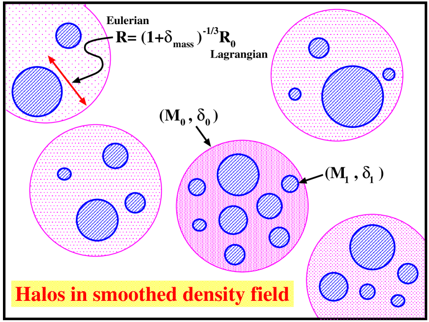
Figure 1: A schematic picture of our halo biasing model at a given redshift $z$. The mass and halo density fields are top-hat smoothed with the Eulerian proper radius $R$, and $R_{0}$ is its Lagrangian counterpart. Each sampling sphere is characterized by $R$ and the Eulerian mass density contrast ${\delta_{\rm mass}}$, or equivalently by the enclosed mass $M_{0}$ and the linearly extrapolated mass density contrast $\delta_{0}$. Within each sampling sphere, there are a number of dark halos characterized by their mass $M_{1}$ and the linearly extrapolated mass density contrast $\delta_{1}$. With a given $z$, $\delta_{1}$ is related to the formation epoch ${z_{\rm f}}$ of the halo.

As illustrated schematically in Figure 1, we consider the mass and galaxy density fields at redshift $z$ smoothed over the top-hat Eulerian proper radius $R$. The mass density contrast ${\delta_{\rm mass}}$ computed in the Eulerian coordinate relates $R$ with its Lagrangian coordinate counterpart $R_{0}=(1+{\delta_{\rm mass}})^{1/3}R$ assuming the spherical collapse. Then the mass in the sphere $M_{0}$ is simply given by $(4\pi/3)\bar{\rho}_{\rm mass}R_{0}^{3}$, where $\bar{\rho}_{\rm mass}(z)$ is the physical mass density at $z$. Also the linearly extrapolated mass density contrast $\delta_{0}$ in the sphere can be evaluated from ${\delta_{\rm mass}}$ on the basis of the nonlinear spherical collapse model (e.g., Mo & White 1996).

Each sphere of the Eulerian radius $R$ should contain a number of gravitationally virialized objects i.e., dark matter halos. Given $M_{0}$ and $\delta_{0}$, their conditional mass function can be predicted by extended Press-Schechter theory (e.g., Bower 1991; Bond et al. 1991). Such halos are conventionally characterized by their mass $M_{1}$ and linearly extrapolated mass density contrast $\delta_{1}$ assuming that their formation epoch is equivalent to the current redshift $z$. Kitayama & Suto (1996a) pointed out that this approximation often significantly changes the predictions for X-ray cluster abundances on the basis of the Press-Schechter theory, and proposed a phenomenological prescription to compute the formation epoch ${z_{\rm f}}$. In fact, the halo biasing derived by Mo & White (1996) is fairly sensitive to the difference of $z$ and ${z_{\rm f}}$ as noticed by Kravtsov & Klypin (1999). Thus we extend the biasing model of Mo and White (1996), in which ${z_{\rm f}}$ should be specified a priori, by considering explicitly the dependence on ${z_{\rm f}}$ and averaging according to the formation epoch distribution function of Lacey & Cole (1993) and Kitayama & Suto (1996b). This is a major and important improvement of our model over the original proposal of Mo and White (1996). In our model, therefore, the formation epoch ${z_{\rm f}}$ and the mass of halo $M_{1}$ constitute the hidden variables $\vec{\cal U}$ (§2), and their PDFs generate the nonlinear and stochastic behavior in the resultant halo biasing.

3.2 Halo biasing from the extended Press-Schechter theory

In what follows, we assume that the primordial mass density field obeys the random - Gaussian statistics (e.g., Bardeen et al. 1986). In this case, the (unconditional) mass function of dark halos (Press & Schechter 1974) :

$$n(M_{1},z;\delta_{1})dM_{1}=\frac{1}{\sqrt{2\pi}}\frac{\bar{\rho}_{\rm mass}}{M_{1}}\frac{\delta_{1}}{\sigma^{3}(M_{1},z)}\exp{\left[-\frac{\delta_{1}^{2}}{2\sigma^{2}(M_{1},z)}\right]}\left|\frac{d\sigma^{2}(M_{1},z)}{dM_{1}}\right|dM_{1}$$ (23)

proves to be in reasonable agreement with results from $N$-body simulations (e.g., Efstathiou et al. 1988; Suto 1993; Lacey & Cole 1993,1994). Equation (23) corresponds to the comoving number density of halos exceeding the critical density threshold $\delta_{1}$ and of mass between $M_{1}$ and $M_{1}+dM_{1}$. The value for $\delta_{1}$ will be specified when we consider the one-point function or the conditional PDF of the dark halos below (see eqs. [28] and [36]). The mass variance $\sigma^{2}(M_{1},z)$ is defined from the linear power spectrum of mass density fluctuations $P_{\rm lin}(k)$ at present ($z=0$):

$$\sigma^{2}(M_{1},z)=D^{2}(z)~{}\int\frac{dk}{2\pi^{2}}~{}k^{2}P_{\rm lin}(k)W^{2}(kR_{1}),$$ (24)

where $D(z)$ is the linear growth factor normalized to unity at $z=0$ and the top-hat window function:

$$W(x)=\frac{3}{x^{3}}(\sin{x}-x\cos{x})$$ (25)

with the Lagrangian radius $R_{1}\equiv(4\pi\bar{\rho}_{\rm mass}/3M_{1})^{-1/3}$ is adopted.

Since our one-point statistics of halos is evaluated within a sample of spheres of the Eulerian radius $R$, we need the conditional mass function for halos within a sphere. For this purpose, we use the extended Press-Schechter theory which predicts the conditional mass function for halos of $(M_{1},~{}\delta_{1})$ and $(M_{1}+dM_{1},~{}\delta_{1})$ in the background region of $(M_{0},~{}\delta_{0})$ as

$$n(M_{1},\delta_{1}|M_{0},\delta_{0};z)dM_{1} = \frac{1}{\sqrt{2\pi}}\frac{\bar{\rho}_{\rm mass}}{M_{1}}\frac{\delta_{1}-\delta_{0}}{[\sigma^{2}(M_{1},z)-\sigma^{2}(M_{0},z)]^{3/2}}$$ (26)

$$\times \exp{\left[-\frac{(\delta_{1}-\delta_{0})^{2}}{2\{\sigma^{2}(M_{1},z)-\sigma^{2}(M_{0},z)\}}\right]}\left|\frac{d\sigma^{2}(M_{1},z)}{dM_{1}}\right|dM_{1}.$$ (27)

Then the biased density field for halos of mass $M_{1}$, which formed at ${z_{\rm f}}$ and are observed at $z$ within the sampling sphere of $(R,{\delta_{\rm mass}})$ in Eulerian coordinates, is derived by Mo & White (1996):

$${\delta_{\rm halo}}={\Delta_{\rm h}}(R,z|~{}{\delta_{\rm mass}},~{}{z_{\rm f}},~{}M_{1})\equiv(1+{\delta_{\rm mass}})\frac{n(M_{1},~{}\delta_{c}(z,{z_{\rm f}})~{}|M_{0},~{}\delta_{0}~{};z)}{n(M_{1},z;\delta_{c}(z,{z_{\rm f}}))}-1.$$ (28)

In the above, the critical threshold $\delta_{c}$ for those halos is given as

$$\delta_{c}(z,{z_{\rm f}})=\delta_{c,0}~{}\frac{D(z)}{D({z_{\rm f}})},\qquad\delta_{c,0}\equiv\frac{3(12\pi)^{2/3}}{20}\simeq 1.69,$$ (29)

again on the basis of the spherical collapse model. The remaining task is to compute the mass, $M_{0}$, and the linearly extrapolated mass density contrast, $\delta_{0}$, of the sampling sphere from its Eulerian radius and density contrast $(R,{\delta_{\rm mass}})$. Since $\delta_{0}\ll 1$, the former is simply given as

$$M_{0}={4\pi\over 3}\,\bar{\rho}_{\rm mass}(z)\,(1+\delta_{0})\,R_{0}^{3}\simeq{4\pi\over 3}\,\bar{\rho}_{\rm mass}(z)\,(1+{\delta_{\rm mass}})\,R^{3},$$ (30)

with $\bar{\rho}_{\rm mass}(z)$ being the physical mass density at $z$. Finally we adopt the following fitting formula obtained in the spherical collapse model (Mo & While 1996) to compute $\delta_{0}$ in terms of ${\delta_{\rm mass}}$:

$$\delta_{0}=\delta_{c,0}-\frac{1.35}{(1+{\delta_{\rm mass}})^{2/3}}+\frac{0.78785}{(1+{\delta_{\rm mass}})^{0.58661}}-\frac{1.12431}{(1+{\delta_{\rm mass}})^{1/2}}.$$ (31)

While equations (29) and (31) were originally derived in the Einstein-de Sitter model, we numerically checked that they provide sufficiently accurate approximations for our present purpose even in the $\Omega_{0}=0.3$ and $\lambda_{0}=0.7$ model that we consider later. Thus we use the expressions (29) and (31) irrespectively of the cosmological models in the subsequent analysis.

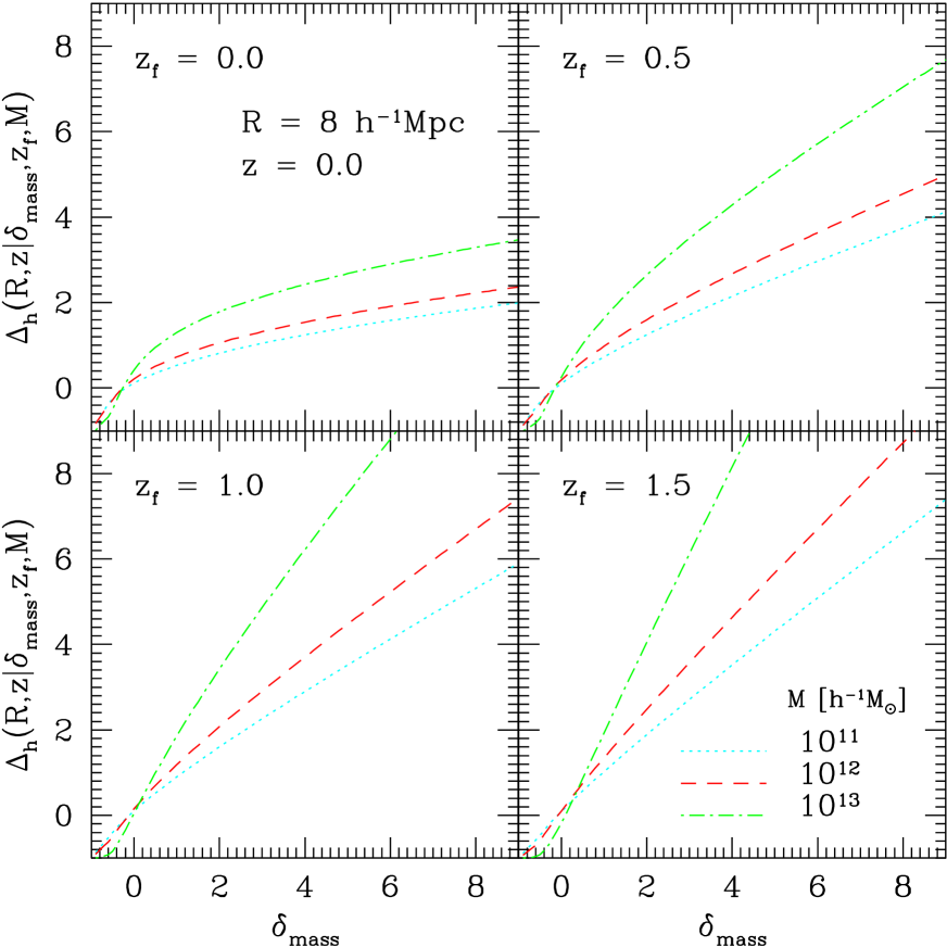
Figure 2: The halo biasing field smoothed over $R=8{\hbox{$h^{-1}$}{\rm Mpc}}$ at $z=0$ as a function of its mass $M$ and formation redshift ${z_{\rm f}}$ in dotted ($M=10^{11}h^{-1}M_{\odot}$), dashed ($M=10^{12}h^{-1}M_{\odot}$), and dot-dashed ($M=10^{13}h^{-1}M_{\odot}$) lines. Upper-left: ${z_{\rm f}}=0$; Upper-right: ${z_{\rm f}}=0.5$; Lower-left: ${z_{\rm f}}=1.0$; Lower-right: ${z_{\rm f}}=1.5$.

Figure 2 illustrates the dependence of ${\Delta_{\rm h}}$ on $M$ and ${z_{\rm f}}$ as a function of ${\delta_{\rm mass}}$ smoothed over $R=8{\hbox{$h^{-1}$}{\rm Mpc}}$ at $z=0$. Given a halo mass, ${\Delta_{\rm h}}$ is very sensitive to the formation epoch ${z_{\rm f}}$ especially in the range of ${z_{\rm f}}\lower 2.15277pt\hbox{$\;\buildrel<\over{\sim}\;$}z+1$. As ${z_{\rm f}}$ increases, the dependence ${\Delta_{\rm h}}$ and $M$ and ${\delta_{\rm mass}}$ becomes significant; this reflects the fact that the larger mass halos preferentially form in the denser regions than the average since the typical halo mass that can be collapsed and virialized decreases at higher ${z_{\rm f}}$. Such $M$ and ${z_{\rm f}}$ dependence of ${\Delta_{\rm h}}$ convolved with the PDF of $M$ and ${z_{\rm f}}$ leads to the nonlinear stochastic behavior of the biasing of dark halos.

While we regard halo mass $M_{1}$ and its formation epoch ${z_{\rm f}}$ as the hidden variables in equation (28), they may not be entirely unobservable. One may infer the halo mass and the formation epoch for an individual galaxy by combing the observed luminosity, color and metallicity with a galaxy evolution model. In this case, their probability distribution functions need to be convolved with such observational selection functions with our prior distribution. Except for this correction, our methodology presented below remains the same.

3.3 Formation epoch distribution of dark halos

As indicated in equation (28), the amplitude of halo biasing is explicitly dependent on its formation epoch ${z_{\rm f}}$. Thus the simple approximation of ${z_{\rm f}}=z$ may lead to even qualitatively incorrect predictions for the biasing. In fact this was shown to be the case in recent N-body simulations by Kravtsov & Klypin (1999). The importance of the distribution of ${z_{\rm f}}$ has been emphasized by Kitayama & Suto (1996a) in a different context, and a model for its PDF was proposed by Lacey & Cole (1993). Incidentally Catelan et al. (1998a,b) also proposed a different model of halo biasing considering the ${z_{\rm f}}$-dependence. Their model simply treats ${z_{\rm f}}$ as a free parameter and does not properly take account of its distribution function. Our model presented here incorporates the distribution function of the formation epoch explicitly.

Adopting the excursion set approach (Bond et al. 1991) and defining the formation redshift ${z_{\rm f}}$ of a particular halo of mass $M$ at $z$ as the epoch when the mass of its most massive progenitor exceeds $M/2$ for the first time, Lacey & Cole (1993) derived the differential distribution of the halo formation epoch $\partial p/\partial{z_{\rm f}}$. Their result is expressed as

$$\frac{\partial p}{\partial{z_{\rm f}}}({z_{\rm f}}~{}|M,~{}z)d{z_{\rm f}}=\frac{\partial p}{\partial\tilde{\omega}_{\rm f}}(\tilde{\omega}_{\rm f},~{}M)~{}\frac{\partial\tilde{\omega}_{\rm f}}{\partial{z_{\rm f}}}d{z_{\rm f}},$$ (32)

$$\frac{\partial p}{\partial\tilde{\omega}_{\rm f}}(\tilde{\omega}_{\rm f},~{}M)=-\frac{1}{\sqrt{2\pi}}\int_{0}^{1}\frac{d\tilde{S}}{\tilde{S}^{3/2}}\frac{M}{M^{\prime}(\tilde{S})}\left(1-\frac{\tilde{\omega}_{\rm f}^{2}}{\tilde{S}}\right)e^{-\tilde{\omega}_{\rm f}^{2}/(2\tilde{S})},$$ (33)

where

$$\tilde{\omega}_{\rm f}({z_{\rm f}},M,z) \equiv \frac{\delta_{c}(z,{z_{\rm f}})-\delta_{c,0}}{\sqrt{\sigma^{2}(M/2,z)-\sigma^{2}(M,z)}},$$ (34)

$$\tilde{S}(M^{\prime},M) \equiv \frac{\sigma^{2}(M^{\prime},z)-\sigma^{2}(M,z)}{\sigma^{2}(M/2,z)-\sigma^{2}(M,z)}.$$ (35)

The function $M^{\prime}(\tilde{S})$ in the integrand of equation (33) can be obtained from equation (35). While the above expressions are rather complicated, practical fitting formulae for the mass variance in cold dark matter (CDM) models and for the formation epoch distribution were obtained in Kitayama & Suto (1996b) which we adopt throughout the analysis. Those are summarized in Appendices A and B for convenience.

It should be noted that the definition of halo formation is somewhat ambiguous in the framework of the extended PS theory. This aspect is explored in Kitayama & Suto (1996a), and their Figure 1 explicitly shows how the result is dependent on the adopted ratio of the current halo mass and the progenitor mass at the formation epoch. The figure implies that the resulting formation rate is fairly insensitive to the value around 0.5 that we adopt here.

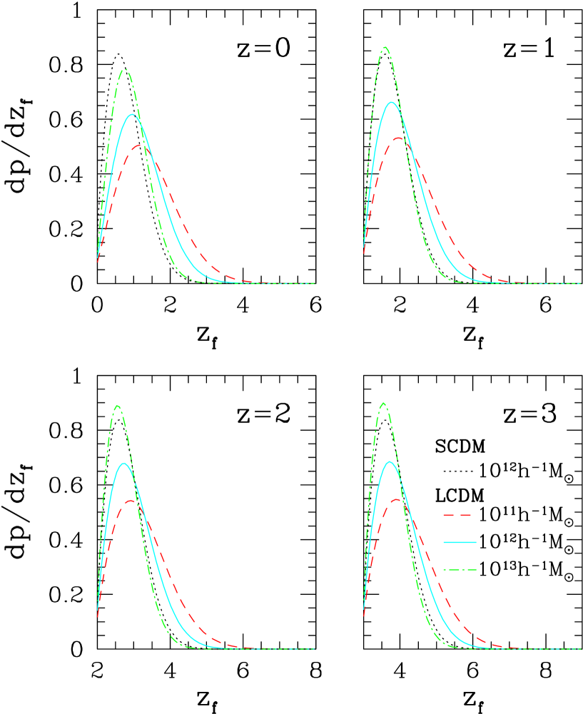
Figure 3: Formation epoch distribution of dark halos. Dotted lines indicate the results for $M=10^{12}h^{-1}M_{\odot}$ in SCDM model, while dashed, solid and dot-dashed lines are respectively for $M=10^{11}h^{-1}M_{\odot}$, $10^{12}h^{-1}M_{\odot}$ and $10^{13}h^{-1}M_{\odot}$ in LCDM model. Upper-left: $z=0$; Upper-right: $z=1$; Lower-left: $z=2$; Lower-right: $z=3$.

Figure 3 plots the formation epoch distribution for halos selected at $z$ in CDM models. Specifically we choose $(\Omega_{0},\lambda_{0},\sigma_{8},h)$ $=(0.7,0.3,1.0,0.7)$ (Lambda CDM; hereafter LCDM ) and $(1.0,0.0,0.6,0.5)$ (Standard CDM; hereafter SCDM). The top-hat mass fluctuation amplitude at $8{\hbox{$h^{-1}$}{\rm Mpc}}$, $\sigma_{8}$, is normalized to the cluster abundance (Kitayama & Suto 1997). We show results for halos of $M=10^{11}h^{-1}{M_{\odot}}$(dashed), $10^{12}{M_{\odot}}$(solid) and $10^{13}h^{-1}{M_{\odot}}$(dot-dashed) in LCDM, and $10^{12}{M_{\odot}}$(dotted) in SCDM. The shape of those distribution functions is quite similar, and characterized by a peak around ${z_{\rm f}}=z+(0.5\sim 1)$. The peak redshift becomes closer to the observed one, $z$, and the distribution around the peak becomes narrower as the halo mass increases, both of which are easily understood in the hierarchical clustering picture like the present models.

Note that the SCDM model generally predicts a more sharply peaked distribution closer to $z$ than the LCDM model (compare solid and dotted lines in Fig.3). This is also reasonable from the fact that the growth of fluctuations is rapid in SCDM and thus halos form only recently. Thus the formation epoch distribution is fairly sensitive to the cosmological parameters.

3.4 Conditional and joint probability distribution functions of dark halos and mass

Now we are in a position to explicitly construct the conditional probability distribution of the dark halo $P({\delta_{\rm halo}}|{\delta_{\rm mass}})$ for a given ${\delta_{\rm mass}}$, and the joint probability distribution $P({\delta_{\rm halo}},{\delta_{\rm mass}})$. Basically we follow the prescription described in §2.1, but in slightly different order.

We first compute $P({\delta_{\rm halo}}|{\delta_{\rm mass}})$ applying equation (10):

$$P({\delta_{\rm halo}}|{\delta_{\rm mass}})~{}d{\delta_{\rm halo}}~{}=~{}{\cal N}^{-1}~{}\int\int_{{\cal C}(M,{z_{\rm f}})}dM~{}d{z_{\rm f}}~{}~{}\frac{\partial p}{\partial{z_{\rm f}}}(z_{f}|M,z)~{}n(M,z;\delta_{c,0}),$$ (36)

where the region ${\cal C}(M,{z_{\rm f}})$ of the integration is determined from the following conditions:

$${\cal C}(M,{z_{\rm f}})=\{~{}(M,{z_{\rm f}})~{}|~{}{\delta_{\rm halo}}\leq~{}{\Delta_{\rm h}}(R,z|{\delta_{\rm mass}},M,{z_{\rm f}})~{}\leq{\delta_{\rm halo}}+d{\delta_{\rm halo}},$$ (37)

$$M_{\rm min}\leq M\leq M_{\rm max},\quad z\leq{z_{\rm f}}\leq\infty~{}\}\hskip 28.45274pt$$ (38)

The normalization factor ${\cal N}$ is defined as

$${\cal N}=\int_{M_{\rm min}}^{M_{\rm max}}dM\int_{z}^{\infty}d{z_{\rm f}}~{}~{}\frac{\partial p}{\partial{z_{\rm f}}}({z_{\rm f}}|M,z)~{}n(M,z;\delta_{c,0}).$$ (39)

The integrand in equation (36) just corresponds to the joint PDF $P(\vec{\cal U}|{\delta_{\rm mass}})$ for a given ${\delta_{\rm mass}}$.

Since the joint PDF is simply computed according to

$$P({\delta_{\rm mass}},{\delta_{\rm halo}})=P({\delta_{\rm halo}}|{\delta_{\rm mass}})\,P({\delta_{\rm mass}}),$$ (40)

one needs a reliable model for the one-point PDF of dark matter density contrast, $P({\delta_{\rm mass}})$. Fortunately it has been known that this can be empirically approximated by the log-normal distribution function to a good accuracy (e.g., Coles & Jones 1991; Kofman et al. 1994; Bernardeau & Kofman 1995; Taylor & Watts 2000):

$$P({\delta_{\rm mass}})\,d{\delta_{\rm mass}}=\frac{1}{\sqrt{2\pi}\sigma_{1}}\exp\left[-\frac{\left\{\ln(1+{\delta_{\rm mass}})+\sigma_{1}^{2}/2\right\}^{2}}{2\sigma_{1}^{2}}\right]\frac{d{\delta_{\rm mass}}}{1+{\delta_{\rm mass}}},$$ (41)

where

$$\sigma_{1}^{2}=\ln(1+\sigma_{\rm mm}^{2}),$$ (42)

and ${\sigma_{\rm mm}}$ is defined in equation (13). Note that equation (41) reduces to the Gaussian distribution for ${\sigma_{\rm mm}}\ll 1$, and thus this model again assumes the primordial random-Gaussian density field implicitly as our entire analysis. Finally we adopt the fitting formula (Peacock & Dodds 1996) for the nonlinear CDM power spectrum $P_{\rm nl}(k,z)$ in computing the mass variance:

$$\sigma_{\rm mm}^{2}(R,z)=\int\frac{dk}{2\pi^{2}}~{}k^{2}P_{\rm nl}(k,z)W^{2}(kR)~{},$$ (43)

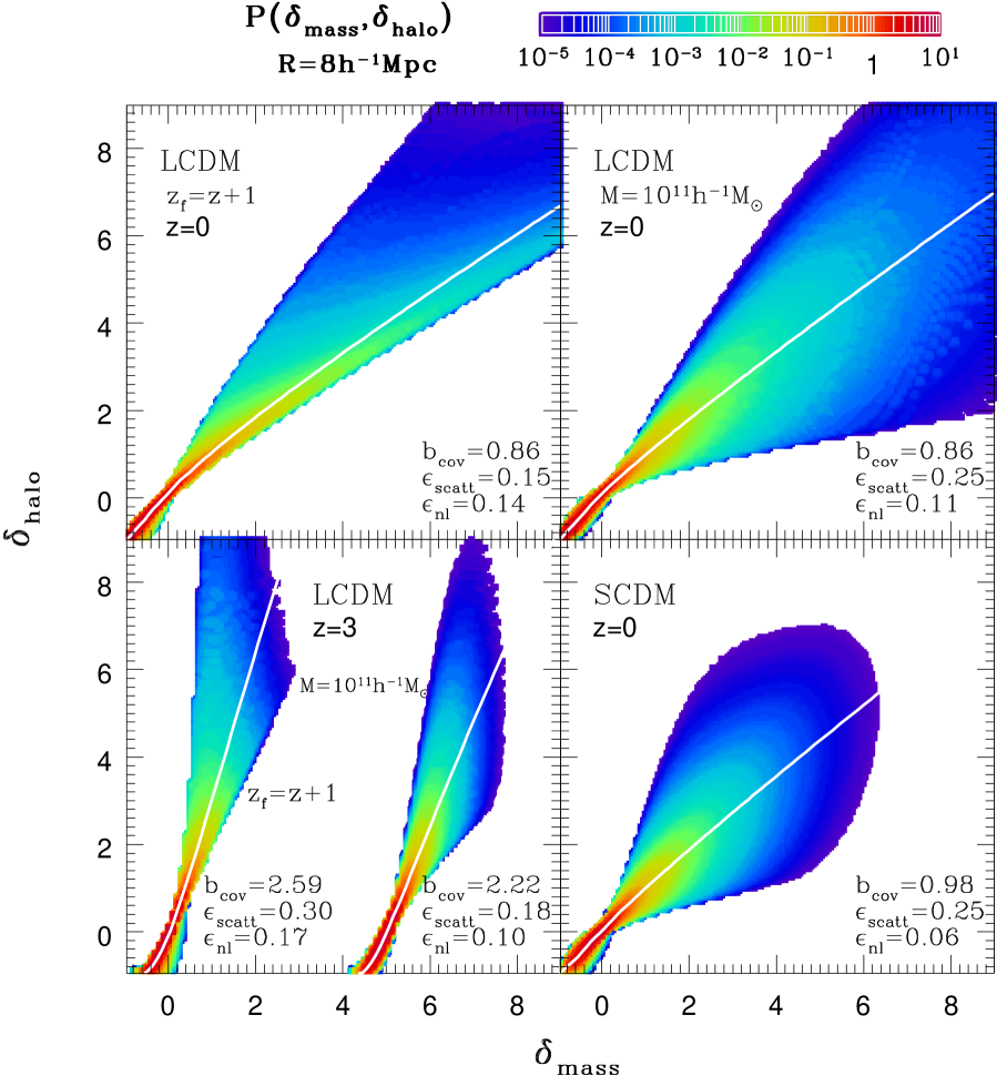
Figure 10: Joint probability distribution of ${\delta_{\rm mass}}$ and ${\delta_{\rm halo}}$, $P({\delta_{\rm mass}},{\delta_{\rm halo}})$ at $R=8h^{-1}$Mpc for different models. Upper-left: LCDM with $z_{\rm f}=z+1$ at $z=0$; Upper-right: LCDM with $M=10^{11}h^{-1}{M_{\odot}}$ at $z=0$; Lower-left: LCDM with $z_{\rm f}=z+1$ and with $M=10^{11}h^{-1}M_{\odot}$ (the value of ${\delta_{\rm mass}}$ is artificially shifted by five for clarity), at $z=3$; Lower-right: SCDM with $10^{11}h^{-1}{M_{\odot}}<M<10^{13}h^{-1}{M_{\odot}}$ at $z=0$.

with $W(kR)$ being the top-hat smoothing function (eq.[25]). The validity of the log-normal approximation for the one-point PDF is examined by Bernardeau & Kofman (1995); their Figure 10 indicates that equation (41) reproduces the simulation results very accurately at least for $R\lower 2.15277pt\hbox{$\;\buildrel>\over{\sim}\;$}5h^{-1}$Mpc. Although the accuracy on smaller scales is not shown quantitatively, it would be reasonable to assume that the approximation is acceptable up to $R\sim 1h^{-1}$Mpc. Also our statistical results are not sensitive to the tail of such PDF in any case.

Substituting the analytical expressions for ${\partial p}/{\partial{z_{\rm f}}}(z_{f}|M,z)$ and $n(M,z;\delta_{c,0})$ discussed in §3.3 into equation (36), one may numerically compute the conditional PDF $P({\delta_{\rm halo}}|{\delta_{\rm mass}})$, and the joint PDF $P({\delta_{\rm halo}},{\delta_{\rm mass}})$ from equation (40). Then all the statistical quantities can be evaluated using equation (8). In practice, however, it is more convenient and even accurate to use (9) which in the present case is written explicitly as

$${\langle\langle}{\cal F}({\delta_{\rm halo}},~{}{\delta_{\rm mass}}){\rangle\rangle} = {\cal N}^{-1}~{}\int_{-1}^{\infty}d{\delta_{\rm mass}}~{}P({\delta_{\rm mass}})$$ (44)

$$\times \left[\int_{M_{\rm min}}^{M_{\rm max}}dM\int_{z}^{\infty}dz_{f}~{}{\cal F}({\Delta_{\rm h}},~{}{\delta_{\rm mass}})~{}\frac{\partial p}{\partial z_{f}}(z_{f}|M,z)~{}n(M,z;\delta_{c,0})~{}\right].$$ (45)

We use the above expression in evaluating the various biasing parameters below except in presenting the PDFs directly.

4 Results in CDM models

We present several specific predictions applying our nonlinear stochastic halo biasing model to representative CDM models mentioned in §3.3. Throughout the analyses, we consider the range of halo mass between $M_{\rm min}=10^{11}h^{-1}{M_{\odot}}$ and $M_{\rm max}=10^{13}h^{-1}{M_{\odot}}$ unless otherwise stated.

The general formulation described in the previous section should work in principle even on fully nonlinear scales. In practice, however, the results presented below are limited by the halo exclusion effect (due to the finite size of halos) and our approximation, equation (41), for the one-point PDF. The validity of both effects should be carefully checked on small scales. Since a typical virial radius of a halo of mass $M$ in LCDM model is $\sim 0.5(M/10^{13}M_{\odot})^{1/3}h^{-1}$ Mpc, the exclusion effect cannot be neglected below $R=1h^{-1}$Mpc but is not so strong for $R\lower 2.15277pt\hbox{$\;\buildrel>\over{\sim}\;$}3h^{-1}$Mpc even for our largest mass considered ($M_{\rm max}=10^{13}h^{-1}{M_{\odot}}$). Also the validity of of the log-normal approximation is already remarked in subsection 3.4. Thus we expect that our predictions below are fairly reliable up to $R\sim 3h^{-1}$Mpc.

4.1 Conditional probability distribution of ${\delta_{\rm mass}}$ and ${\delta_{\rm halo}}$

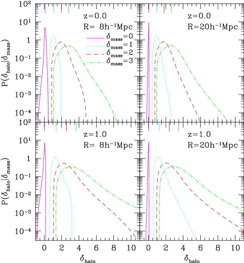
Figure 4: Conditional probability of ${\delta_{\rm halo}}$ for ${\delta_{\rm mass}}=0$ (solid), $1$ (dotted), $2$ (dashed) and $3$ (dot-dashed) in LCDM model for $10^{11}h^{-1}M_{\odot}<M<10^{13}h^{-1}M_{\odot}$. Upper-left: $z=0$ and $R=8h^{-1}$Mpc; Upper-right: $z=0$ and $R=20h^{-1}$Mpc; Lower-left: $z=1$ and $R=8h^{-1}$Mpc; Lower-right: $z=1$ and $R=20h^{-1}$Mpc.

Since the conditional PDF $P({\delta_{\rm halo}}|{\delta_{\rm mass}})$ plays a central role in the Dekel & Lahav (1999) description of the nonlinear stochastic biasing, we first present $P({\delta_{\rm halo}}|{\delta_{\rm mass}})$ predicted from our model. For this purpose, we start with equations (36) and (37). Specifically we divide the $({\delta_{\rm gal}},{\delta_{\rm mass}})$ plane in a $3000\times 3000$ mesh, and accumulate the integrand of equation (36) satisfying the constraint (37) on each grid. The resulting PDFs are plotted in Figure 4 for a given mass density contrast; ${\delta_{\rm mass}}=0$ (solid), ${\delta_{\rm mass}}=1$ (dotted), ${\delta_{\rm mass}}=2$ (dashed) and ${\delta_{\rm mass}}=3$ (dot-dashed). The upper and lowers panels show the results at $z=0$ and $z=1$, respectively, with the top-hat smoothing radius of $R=8h^{-1}$Mpc (left) and $R=20h^{-1}$Mpc (right).

The ticks on the upper axis in each panel indicate the corresponding conditional mean $\overline{\delta_{\rm halo}}$ (eq.[15]). The peak position of the distribution is in reasonable agreement with $\overline{\delta_{\rm halo}}$. As Figure 2 indicates, ${\Delta_{\rm h}}$ given $z$ and $R$ is fairly monotonically dependent on $M$ and ${z_{\rm f}}$. Thus the peak in the conditional PDF reflects that of the formation epoch distribution $\partial p/\partial{z_{\rm f}}$. The width of the distribution around the peak, on the other hand, is dominated by the mass distribution since ${\Delta_{\rm h}}$ becomes more sensitive to the halo mass in a denser environment (Fig.2).

4.2 Joint probability distribution of ${\delta_{\rm mass}}$ and ${\delta_{\rm halo}}$

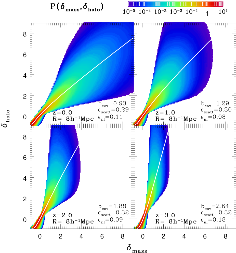
Figure 5: Contour plot of the joint probability distribution of ${\delta_{\rm mass}}$ and ${\delta_{\rm halo}}$, $P({\delta_{\rm mass}},{\delta_{\rm halo}})$. These examples are for $10^{11}h^{-1}M_{\odot}<M<10^{13}h^{-1}M_{\odot}$ and $R=8h^{-1}$Mpc in LCDM model. Upper-left: $z=0$; Upper-right: $z=1$; Lower-left: $z=2$; Lower-right: $z=3$.

Once $P({\delta_{\rm halo}}|{\delta_{\rm mass}})$ is given, the joint PDF $P({\delta_{\rm mass}},{\delta_{\rm halo}})$ is simply obtained by multiplying the one-point PDF of the mass density $P({\delta_{\rm mass}})$, in our case, the log-normal model (eq.[41]). The resulting contour on $({\delta_{\rm mass}},{\delta_{\rm halo}})$ plane is illustrated in Figure 5. This example shows the result with the top-hat smoothing radius of $R=8h^{-1}$Mpc at different redshifts. Solid lines in each panel indicate the conditional mean $\overline{\delta_{\rm halo}}({\delta_{\rm mass}})$.

The number density of halos of mass exceeding the current threshold $M_{\rm min}=10^{11}h^{-1}{M_{\odot}}$ become progressively smaller as $z$ increases. Such halos naturally reside in higher density regions, and therefore are strongly biased with respect to mass. The biasing of those halos gradually decreases as time since they simply follow the gravitational field of the background mass after formation (Fry 1996; Tegmark & Peebles 1998; Taruya, Koyama & Soda 1999). In addition, new halos with $M>M_{\rm min}$ form more easily later and can be found even at moderately dense environment. For both reasons, the mean bias $\overline{\delta_{\rm halo}}$ as a function of ${\delta_{\rm mass}}$ decreases at lower redshifts.

At $z=0$, the joint PDF $P({\delta_{\rm mass}},{\delta_{\rm halo}})$ shows slightly anti-biasing behavior, i.e, $\overline{\delta_{\rm halo}}\lower 2.15277pt\hbox{$\;\buildrel<\over{\sim}\;$}{\delta_{\rm mass}}$. This is partly due to the fact that a fraction of halos with $M<M_{\rm max}$ are merged into a part of larger mass halos since the typical virialized halo mass $M_{*}(z)$ at $z=0$ approaches the mass scale $M_{0}(R)$, corresponding to our adopted smoothing radius $R=8h^{-1}$Mpc itself. In other words, our halo model generally predicts the positive-biasing except for those halos of $M\lower 2.15277pt\hbox{$\;\buildrel<\over{\sim}\;$}M_{*}(z)\lower 2.15277pt\hbox{$\;\buildrel<\over{\sim}\;$}M_{0}(R)$ for given $R$ and $z$.

While Figure 5 elucidates the global feature of the joint PDF, the statistical weights are practically dominated by the relatively narrow regions around ${\delta_{\rm halo}}\sim\overline{\delta_{\rm halo}}({\delta_{\rm mass}})$. Those regions are illustrated better in logarithmic scales rather than in linear scales. For this purpose, we recompute the joint PDF from equations (36) and (37) using the $3000\times 3000$ mesh with the logarithmically equal bin on the $(1+{\delta_{\rm gal}},1+{\delta_{\rm mass}})$ plane. Note that the resulting PDF sampled in this way, $\tilde{P}(1+{\delta_{\rm mass}},1+{\delta_{\rm halo}})$, satisfies

$$\tilde{P}(1+{\delta_{\rm mass}},1+{\delta_{\rm halo}})\,d\ln(1+{\delta_{\rm mass}})\,d\ln(1+{\delta_{\rm halo}})=P({\delta_{\rm mass}},{\delta_{\rm halo}})\,d{\delta_{\rm mass}}\,d{\delta_{\rm halo}}.$$ (46)

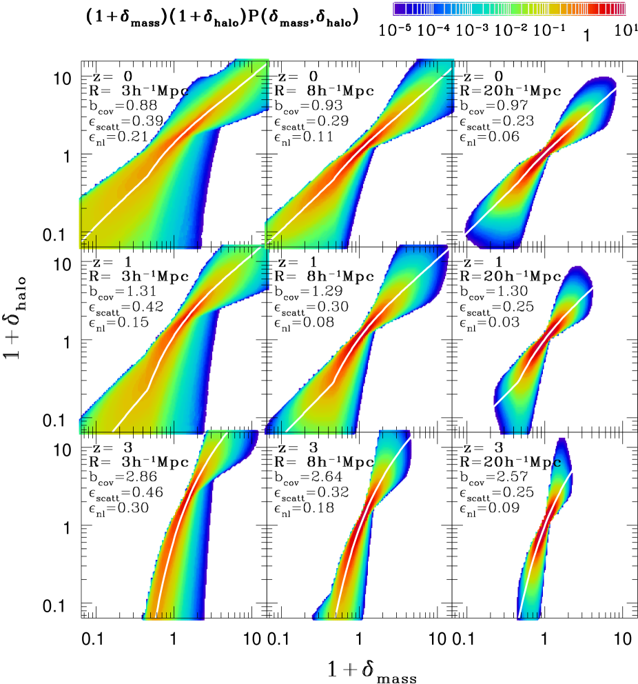
Figure 6: Contour plot of the joint probability distribution of $\tilde{P}(1+{\delta_{\rm mass}},1+{\delta_{\rm halo}})=(1+{\delta_{\rm mass}})(1+{\delta_{\rm halo}})P({\delta_{\rm mass}},{\delta_{\rm halo}})$. These examples are for $10^{11}h^{-1}M_{\odot}<M<10^{13}h^{-1}M_{\odot}$ in LCDM model. The redshifts $z$ are $0$, $1$ and $3$ from top to bottom, and the smoothing lengths $R$ are $3h^{-1}$Mpc, $8h^{-1}$Mpc and $20h^{-1}$Mpc from left to right.

Thus we decide to plot the joint PDF $(1+{\delta_{\rm mass}})(1+{\delta_{\rm halo}})\,P({\delta_{\rm mass}},{\delta_{\rm halo}})$. In Figure 6, the dispersion around the mean biasing decreases at higher $z$ and/or larger $R$ in contrast to the conditional PDF plotted in Figure 4. This is basically because the PDF $P({\delta_{\rm mass}})$ in linear regime becomes toward Gaussian and sharply peaked.

We remark that the contours of our joint PDF plotted in Figures 5 and 6 seem to be very narrow around ${\delta_{\rm mass}}\sim{\delta_{\rm halo}}\sim 0$. This can be understood by the fact that the positive halo density contrast preferentially developed on the over-dense dark matter environment. In other words, this is a natural consequence of our bias model in which the signs of ${\delta_{\rm halo}}$ and ${\delta_{\rm mass}}$ are almost the same as illustrated in Figure 2. Incidentally this feature may be visually exaggerated by the contours of very small probabilities; if one focuses only on the contours of $P({\delta_{\rm mass}},{\delta_{\rm halo}})>0.01$, the effect does not look so strong. In reality, and thus in numerical simulations, additional stochastic processes other than the mass and formation epoch distribution (including the dynamical motion of halos) should further increase the scatter which makes the contour rounder than our predictions.

We will return to these contour plots in understanding the behavior of the biasing parameters later.

4.3 Scale-dependence

The previous two subsections show that the joint and the conditional PDFs are dependent on both $R$ and $z$. This dependence is translated to the scale-dependence and redshift evolution of the second order statistics defined in §2.2.

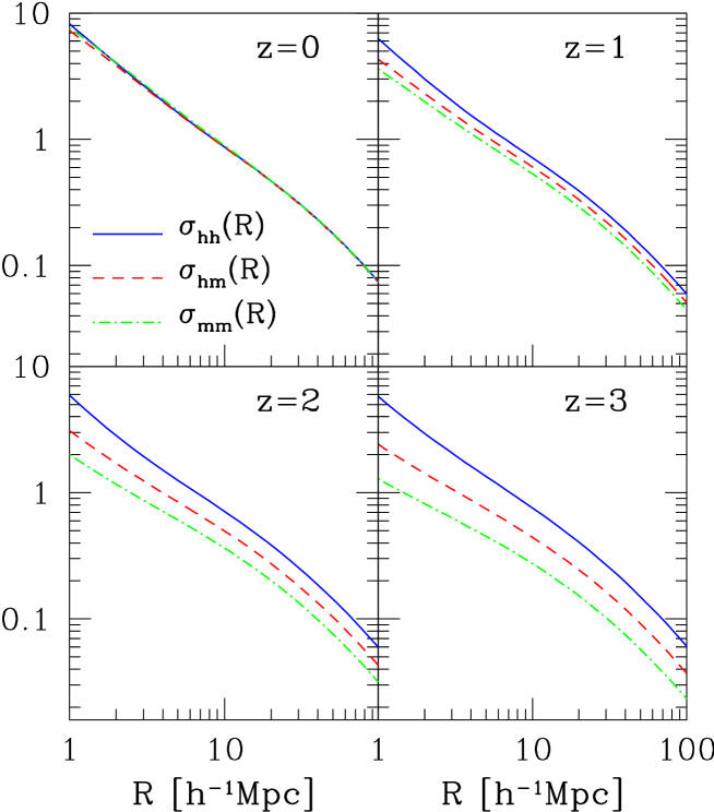
Figure 7: Scale-dependence of $\sigma_{\rm hh}$ (solid), $\sigma_{\rm hm}$ (dashed), and $\sigma_{\rm mm}$ (dot-dashed) at different redshifts; Upper-left: $z=0$; Upper-right: $z=1$; Lower-left: $z=2$; Lower-right: $z=3$.

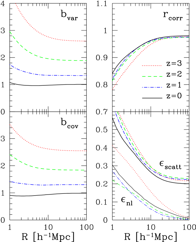
Figure 8: Scale-dependence of biasing parameters, ${b_{\rm var}}$, ${r_{\rm corr}}$, ${b_{\rm cov}}$, ${\epsilon_{\rm scatt}}$ and ${\epsilon_{\rm nl}}$, at the different redshifts $z=0$ (solid), $z=1$ (dot-dashed), $z=2$ (dashed), and $z=3$ (dotted). In the Lower-right panel, thick and thin lines indicate the degree of stochasticity ${\epsilon_{\rm scatt}}$, and nonlinearity ${\epsilon_{\rm nl}}$, respectively.

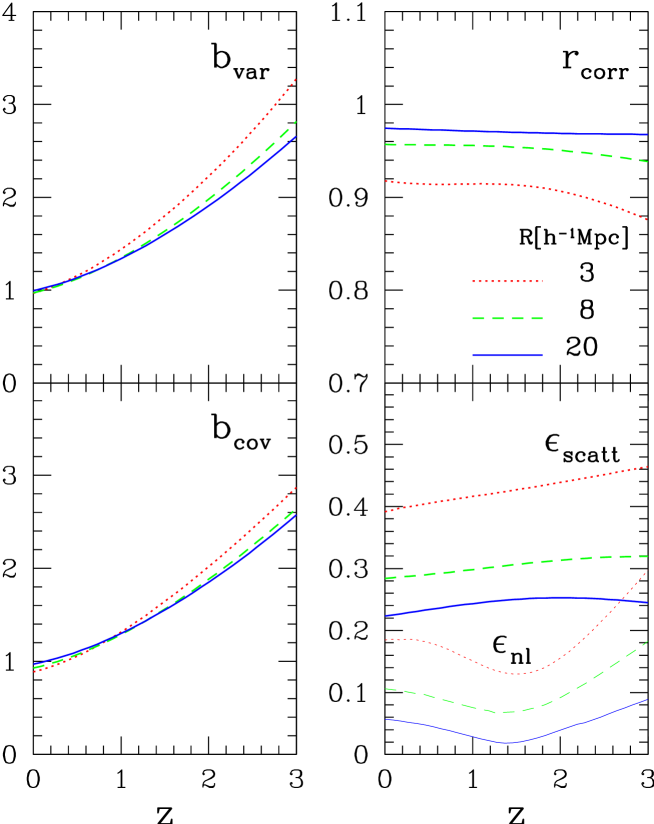
Figure 9: Evolution of biasing parameters, ${b_{\rm var}}$, ${r_{\rm corr}}$, ${b_{\rm cov}}$, ${\epsilon_{\rm scatt}}$ and ${\epsilon_{\rm nl}}$, at $R=3{\hbox{$h^{-1}$}{\rm Mpc}}$ (dotted), $8{\hbox{$h^{-1}$}{\rm Mpc}}$ (dashed), and $20{\hbox{$h^{-1}$}{\rm Mpc}}$ (solid). In the Lower-right panel, thick and thin lines indicate the degree of stochasticity ${\epsilon_{\rm scatt}}$, and nonlinearity ${\epsilon_{\rm nl}}$, respectively.

Figure 7 shows ${\sigma_{\rm hh}}$, ${\sigma_{\rm hm}}$ and ${\sigma_{\rm mm}}$ at different redshifts as a function $R$. We compute those statistics directly integrating equation (44) over $M$, ${z_{\rm f}}$ and ${\delta_{\rm mass}}$, instead of using $P({\delta_{\rm mass}},{\delta_{\rm halo}})$. While their scale- and time-dependence is noticeable even from those panels, the biasing parameters (${b_{\rm var}}$, ${r_{\rm corr}}$, ${b_{\rm cov}}$, ${\epsilon_{\rm scatt}}$ and ${\epsilon_{\rm nl}})$ plotted in Figures 8 and 9 are more suitable in understanding the origin of the behavior.

Consider first the scale-dependence (Fig.8). While ${b_{\rm var}}$ and ${b_{\rm cov}}$ are generally a decreasing function of $R$, this behavior is significant only up to $R\lower 2.15277pt\hbox{$\;\buildrel<\over{\sim}\;$}2(1+z){\hbox{$h^{-1}$}{\rm Mpc}}$ in this model. This feature is more quantitatively exhibited by ${\epsilon_{\rm nl}}$ and ${\epsilon_{\rm scatt}}$ (Lower-right panel). Therefore in practice the linear biasing provides a good approximation on linear and quasi-linear regimes. The biasing is non-deterministic especially on smaller scales almost independently of $z$ (see also Fig.9). In addition, ${r_{\rm corr}}$ does not approach unity even on large scales, implying that non-deterministic nature still exists there to some extent. As the lower-right panel in Figure 8 indicates, ${\epsilon_{\rm scatt}}\gg{\epsilon_{\rm nl}}$ on all scales and the above feature should be ascribed to the stochasticity due to the distribution of $M$ and ${z_{\rm f}}$. In fact, this stochasticity on large scales is expressed explicitly in terms of the linear biasing approximation by Mo & White (1996):

$${\delta_{\rm halo}}\simeq b_{{\scriptscriptstyle{\rm MW}}}~{}{\delta_{\rm mass}},\qquad b_{{\scriptscriptstyle{\rm MW}}}(z|M,{z_{\rm f}})=1+\frac{\nu^{2}-1}{\delta_{c}(z,{z_{\rm f}})},$$ (47)

with $\nu\equiv\delta_{c}(z,{z_{\rm f}})/\sigma(M,z)$. It should be noted that $b_{{\scriptscriptstyle{\rm MW}}}$ is often regarded as a function of $z$ and $M$ assuming $z={z_{\rm f}}$, leading to the linear deterministic model. Thus once a halo mass $M$ is specified, ${\epsilon_{\rm scatt}}=0$. In equation (47), however, we explicitly keep the ${z_{\rm f}}$-dependence which adds the stochastic nature in the model. More specifically, the definition (19) with equations (44) and (47) reduces to

$${\epsilon_{\rm scatt}}^{2}=\frac{{\langle\langle}{\delta_{\rm mass}}^{2}{\rangle\rangle}\,{\langle\langle}(b_{{\scriptscriptstyle{\rm MW}}}{\delta_{\rm mass}}-{\langle\langle}b_{{\scriptscriptstyle{\rm MW}}}{\rangle\rangle}_{M,{z_{\rm f}}}{\delta_{\rm mass}})^{2}{\rangle\rangle}}{{\langle\langle}{\langle\langle}b_{{\scriptscriptstyle{\rm MW}}}{\rangle\rangle}_{M,{z_{\rm f}}}{\delta_{\rm mass}}^{2}{\rangle\rangle}^{2}}=\frac{{\langle\langle}b_{{\scriptscriptstyle{\rm MW}}}^{2}{\rangle\rangle}_{M,{z_{\rm f}}}}{{\langle\langle}b_{{\scriptscriptstyle{\rm MW}}}{\rangle\rangle}_{M,{z_{\rm f}}}^{2}}-1,$$ (48)

where ${\langle\langle}\cdots{\rangle\rangle}_{M,{z_{\rm f}}}$ denotes the average over $M$ and ${z_{\rm f}}$. This accounts for the scale-independent non-vanishing ${\epsilon_{\rm scatt}}$ exhibits in Figure 8. In conclusion, our model implies that the halo biasing does not become fully deterministic even on large scales where its nonlinearity is negligible. This result is not surprising since we take into account the stochastic processes which do not vanish on large scales, but the overall effect is quite small (${r_{\rm corr}}\sim 0.98$).

4.4 Redshift dependence

Next discuss the redshift dependence of our biasing model. Figure 9 shows that ${b_{\rm var}}$ and ${b_{\rm cov}}$ strongly evolve in time. In fact, this is in marked contrast with predictions on the basis of phenomenological linear deterministic models. For example, a model of Fry (1996) leads to evolution of a form:

$$b(z)=1+{1\over D(z)}[b(z=0)-1].$$ (49)

This implicitly assumes that all the objects of interest form at the same ${z_{\rm f}}$ and that their biasing parameters at ${z_{\rm f}}$ are independent of the mass. Since neither the above assumptions apply to our model, the prediction (49) is quite different from ours even in the linear regime. Our results generally show much stronger evolution as $z$ increases despite the fact that $b(z=0)$ is very close to unity. The recent compilation of the various galaxy catalogs also indicates that the prediction (49) does not reasonably describe the behavior at $z\lower 2.15277pt\hbox{$\;\buildrel>\over{\sim}\;$}2$ (Magliocchetti et al. 1999). Thus, the proper modeling in the framework of the nonlinear stochastic biasing is important even in predicting ${b_{\rm var}}$ and ${b_{\rm cov}}$.

In our halo biasing model, the degree of stochasticity ${\epsilon_{\rm scatt}}$ is almost constant in time because it is determined by the effective widths of the probability distribution functions of $M$ and ${z_{\rm f}}$. Incidentally the nonlinearity ${\epsilon_{\rm nl}}$ does not evolve monotonically (thin lines in the Lower-right panel). At an intermediate redshift, ${\epsilon_{\rm nl}}$ reaches at a minimum. This behavior is qualitatively explained from the curvature of the conditional mean $\overline{\delta_{\rm halo}}$ as a function of ${\delta_{\rm mass}}$, i.e., its second derivative $d^{2}\overline{\delta_{\rm halo}}/d{\delta_{\rm mass}}^{2}$. At ${\delta_{\rm mass}}\gg 1$, halos of the mass $M_{\rm min}<M<M_{\rm max}$ that we adopt here exhibit stronger positive biasing ($\overline{\delta_{\rm halo}}>{\delta_{\rm mass}}$) on average at $z\lower 2.15277pt\hbox{$\;\buildrel>\over{\sim}\;$}2$ and mildly anti-biasing ($\overline{\delta_{\rm halo}}\lower 2.15277pt\hbox{$\;\buildrel<\over{\sim}\;$}{\delta_{\rm mass}}$) at $z\lower 2.15277pt\hbox{$\;\buildrel<\over{\sim}\;$}1$. Since ${\delta_{\rm halo}}=-1$ at ${\delta_{\rm mass}}=-1$ by definition (cf., eq.[28]), the dependence results in positive and negative curvatures of $\overline{\delta_{\rm halo}}({\delta_{\rm mass}})$, respectively at $z\lower 2.15277pt\hbox{$\;\buildrel>\over{\sim}\;$}2$ and $z\lower 2.15277pt\hbox{$\;\buildrel<\over{\sim}\;$}1$, especially around ${\delta_{\rm mass}}\sim 0$ where the contribution of the joint PDF $P({\delta_{\rm mass}},{\delta_{\rm halo}})$ is significant. This feature is clearly visible in Figure 5. In turn, the curvature should be minimum somewhere between $z=1$ and $2$. When higher-order correction is neglected, ${\epsilon_{\rm nl}}$ is dominated by the curvature or the second derivative of $\overline{\delta_{\rm halo}}({\delta_{\rm mass}})$ properly averaged over ${\delta_{\rm mass}}$ (eq.[18]), and it should become minimum at the same redshift. It is interesting to note that the qualitatively similar evolutionary feature was found from the numerical simulations of Somerville et al. (2000; their Fig.17).

4.5 Origin of stochasticity and cosmological model dependence

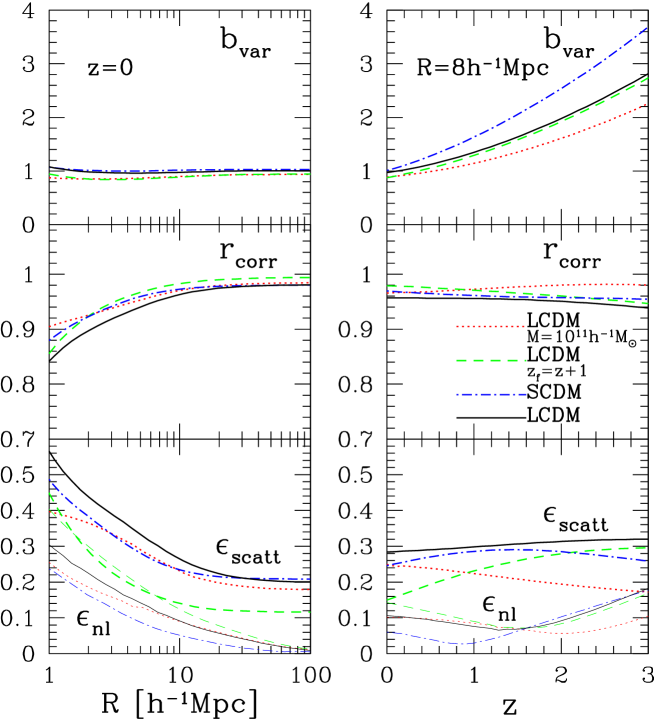
Figure 11: Comparison of ${b_{\rm var}}$, ${r_{\rm corr}}$, ${\epsilon_{\rm scatt}}$ and ${\epsilon_{\rm nl}}$ in different models. Left: at $z=0$; Right: at $R=8{\hbox{$h^{-1}$}{\rm Mpc}}$. Different lines indicate results for LCDM with $M=10^{11}h^{-1}M_{\odot}$ (dotted), LCDM with $z_{\rm f}=z+1$ (dashed), and SCDM with $10^{11}h^{-1}M_{\odot}<M<10^{13}h^{-1}M_{\odot}$ (dot-dashed), in comparison with our canonical model (LCDM with $10^{11}h^{-1}M_{\odot}<M<10^{13}h^{-1}M_{\odot}$) plotted in solid lines.

So far we have presented model predictions for halos averaged over $10^{11}h^{-1}M_{\odot}<M<M^{13}h^{-1}M_{\odot}$ in LCDM model taking into account the appropriate ${z_{\rm f}}$ distribution. Figures 10 and 11 compare those fiducial results with predictions based on the different model assumptions.

First we address the question of the origin of the stochasticity. Since our biasing model has two hidden parameters, $M$ and ${z_{\rm f}}$, we attempt to separate the two sources by fixing $M=10^{11}h^{-1}M_{\odot}$ or ${z_{\rm f}}=z+1$ while keeping the other parameters exactly the same. The upper-panels and the lower-left panel of Figure 10 suggest that the ${z_{\rm f}}$ distribution dominates the stochasticity at low redshift $(z=0)$, while the effect of the $M$ distribution becomes significant at higher redshift $(z=3)$. The same behaviors can be seen in the lower-right panel of Figure 11. Since our model relies on the hierarchical picture of structure formation, the result is simply deduced from the merging history of halos. Thus, in general, the major contribution to the joint PDF can become the formation epoch distribution. This is also indicated in the scale-dependence of the stochasticity in the lower-left panel of Figure 11(thick-dashed and thick-dotted lines).

Next consider the cosmological model dependence. For this purpose, we plot the result in the SCDM model with the same mass range. The joint PDF at $z=0$ and $R=8{\hbox{$h^{-1}$}{\rm Mpc}}$ (Lower-right panel of Fig.10) is confined in a slightly narrower regime compared with that in LCDM. This comes from the fact that the formation epoch in SCDM shows a bit more sharply peaked distribution $\partial p/\partial{z_{\rm f}}$ in than that in LCDM with the same halo mass $M$ (Fig.3). As a result, the stochasticity in SCDM is smaller (i.e., ${\epsilon_{\rm scatt}}$ is smaller and ${r_{\rm corr}}$ is closer to unity), but ${b_{\rm var}}$ at $z=0$ is almost insensitive to such small changes. Rather the major difference between LCDM and SCDM is the redshift evolution of ${b_{\rm var}}$ which increases more rapidly in SCDM reflecting the faster growth rate of density fluctuations.

4.6 Comparison with previous results

Dark matter halos are quite natural and likely sites for galaxy and cluster formation. Thus there are many previous papers to discuss different aspects of the halo biasing on the basis of different assumptions and modeling (Catelan et al. 1999a,b; Blanton et al. 1999). Among others, Kravtsov & Klypin (1999) and Somerville et al. (2000) analyzed the nonlinearity and stochasticity in halo and galaxy biasing using numerical simulations. In this sense their work is complementary to our analytical modeling, and deserves quantitative comparison with our results.

Kravtsov & Klypin (1999) performed high-resolution N-body simulations employing $N=256^{3}$ particles in a periodic $60{\hbox{$h^{-1}$}{\rm Mpc}}$ box so as to overcome the halo over-merging. In particular, their Figure 4 plotting the joint PDF $P({\delta_{\rm mass}},{\delta_{\rm halo}})$ is quite relevant for the comparison with our Figure 5. Strictly speaking, their simulated halo catalogue is based on slightly different identification scheme (Klypin et al. 1999); the bound density maxima algorithm, a selected mass range $[M_{\rm min},M_{\rm max}]$ is limited both by the numerical resolution (individual particle mass) and the simulation boxsize. Furthermore their statistics is based on the smoothing length $R=5h^{-1}$Mpc. Despite such quantitative difference, both contours look surprisingly similar. They pointed out that the Mo & White biasing with ${z_{\rm f}}=z+1$ phenomenologically fits the conditional mean $\overline{\delta_{\rm halo}}({\delta_{\rm mass}})$ of their simulations. Actually this is exactly what we find here, and mainly due to the fairly strong peak in the formation epoch distribution (Fig. 3).

Somerville et al. (2000) examined the nonlinear and stochastic nature in the galaxy biasing combining N-body simulations and semi-analytic model of galaxy formation (see also Kauffmann, Nusser & Steinmetz 1997). While their model incorporates many detailed astrophysical processes (gas cooling, star formation, stellar evolution and population synthesis, galaxy feedback and merging among others) that our analytical modeling neglects, their overall conclusion is that the massive halos ($M\lower 2.15277pt\hbox{$\;\buildrel>\over{\sim}\;$}10^{11}h^{-1}M_{\odot}$) identified from simulations have nearly one-to-one correspondence with luminous galaxies. Their conclusion is encouraging to us since it justifies our crucial assumption that the nonlinearity and stochasticity in the halo biasing are originated mainly from gravitational clustering. In fact, their Figs. 5 and 6 are also very similar to our joint PDF plotted in Figure 6. Furthermore they find (their Fig.17) that both nonlinearity and stochasticity of galaxies evolve moderately as redshift, and decrease on larger scales, and that the stochasticity shows a minimum at an intermediate redshift. These findings are fully consistent with our results and in fact can be explained physically in the framework of our analytic description.

5 Discussion and Conclusions

In this paper, we presented a general formalism to describe the nonlinear stochastic biasing from the hidden variable interpretation. According to this formulation we proposed a physical model for the halo biasing assuming that mass and formation epoch of dark halos act as the major hidden variables. In particular, this model for the first time provides an analytic expression for the joint probability distribution function of the halos and the dark matter density fields. The specific functional forms for the PDFs can be derived, or are at least consistent with the phenomenological results, from the standard gravitational instability theory and the assumption of the random-Gaussianity of the primordial density field. Therefore we expect that the basic features of the nonlinear and stochastic biasing predicted from our model are fairly generic. In fact, detailed comparison with the previous numerical simulations by Kravtsov & Klypin (1999) and Somerville et al. (2000) shows good agreement with our predictions, indicating that the nonlinear and stochastic nature of the halo biasing is essentially understood by taking account of the distribution of the halo mass and the formation epoch.

Then we introduced a set of biasing parameters from second-order statistical quantities following Dekel & Lahav (1999), which properly quantify the one-point statistics of nonlinear and stochastic biasing. As specific examples, we explicit compute those parameters in LCDM model, and examined their scale- and time-dependence. Our major findings are summarized as follows:

1. The biasing of the variance, ${b_{\rm var}}\equiv\sqrt{{\sigma_{\rm hh}}/{\sigma_{\rm mm}}}$, evolves strongly as redshift. While its scale-dependence becomes noticeable on small scales and/or at high redshifts, a simple linear biasing model provides a reasonable approximation roughly at $R\lower 2.15277pt\hbox{$\;\buildrel>\over{\sim}\;$}2(1+z){\hbox{$h^{-1}$}{\rm Mpc}}$.

2. The stochasticity, ${r_{\rm corr}}\equiv{\sigma_{\rm hm}}^{2}/\sqrt{{\sigma_{\rm hh}}{\sigma_{\rm mm}}}$ exhibits moderate scale-dependence especially on $R\lower 2.15277pt\hbox{$\;\buildrel<\over{\sim}\;$}20{\hbox{$h^{-1}$}{\rm Mpc}}$, but is almost independent of $z$. Since ${\epsilon_{\rm scatt}}\gg{\epsilon_{\rm nl}}$ in general, the stochasticity of halo biasing is mainly generated by the scatter which is dominated by the formation epoch distribution at lower redshifts and by the halo mass distribution at higher redshifts. Importantly, the stochasticity still remains constant even on large scales, which yields the small deviation of ${r_{\rm corr}}$ from unity.

The fact that biasing approaches linear and scale-independent on large scales is just expected from previous theoretical work (e.g., Coles 1993; Scherrer & Weinberg 1998) and was recently suggested observationally (Seaborne et al. 1999). Our model further implies that the scale-independence still holds even in the quasi-linear regime, and more importantly, that biasing is still stochastic to some extent on those scales.

Before closing we would like to comment on several limitations of our model and on future prospects in order. First, our analysis is entirely dependent on the formation redshift distribution derived by Lacey & Cole (1993). It is known, however, that the distribution becomes negative in some models, suggesting that this function is not fully correct. Another proposal for the distribution function by Kitayama & Suto (1996a) also suffers from a different conceptual problem. This might be ascribed to the difficulty of distinguishing the merger and accretion unambiguously within the framework of the extended PS theory. Despite this limitation, the two proposals by Lacey & Cole (1993) and by Kitayama & Suto (1996a) lead to very similar predictions and thus we believe it unlikely that this significantly affects the final results. Second, several authors have claimed that a better agreement with numerical simulations is attained by incorporating the non-spherical effect into the Press-Schechter theory (Lee & Shandarin 1998; Sheth, Mo, & Tormen 1999). Although we do not think that the non-spherical effect drastically changes the statistical predictions of our model, this is definitely a well-defined and interesting possibility to improve our model provided that the corresponding distribution function of the formation epoch can be derived. Third, for the proper comparison with observation, our predictions should be corrected for the redshift-space distortion. Since the distortion induced by peculiar velocity field also leads to the stochasticity, the resulting biasing becomes object-dependent (Taruya et al. 2000). Finally and more importantly, the astrophysical effects other than gravity must be taken into account. Since a halo identified in our scheme carries its formation epoch, it is not so difficult to combine with the phenomenological galaxy formation model. Such an improved model will enable more generic and testable predictions for the galaxy biasing.

A.T. gratefully acknowledges support from a JSPS (Japan Society for the Promotion of Science) fellowship. Numerical computations were carried out at RESCEU (Research Center for the Early Universe, University of Tokyo) and ADAC (the Astronomical Data Analysis Center) of the National Astronomical Observatory, Japan. This research was supported in part by the Grant-in-Aid by the Ministry of Education, Science, Sports and Culture of Japan (07CE2002) to RESCEU.

Appendices

Appendix A Mass variance for the CDM model

The mass variance $\sigma(M,z=0)$ defined by equation (24) requires the linear power spectrum of density fluctuations $P_{\rm lin}(k)$. The fitting form of the CDM power spectrum is given by Bardeen et al. (1986) with the scale-invariant Harrison-Zel’dovich initial condition:

$$P_{\rm lin}(k)\propto k\left[\ln(1+2.34q)\over 2.34q\right]^{2}\left[1+3.89q+(16.1q)^{2}+(5.46q)^{3}+(6.71q)^{4}\right]^{-1/2},$$ (A1)

where $q\equiv k/(\Gamma h\mbox{ Mpc}^{-1})$. Here, we adopt $\Gamma=\Omega_{0}h\exp(-\Omega_{\rm b}-\sqrt{2h}\Omega_{\rm b}/\Omega_{0})$ with the baryon density parameter $\Omega_{\rm b}=0.02h^{-2}$.

Numerical integration of equation (24) is straightforward, but time-consuming since we heavily use $\sigma^{2}$ as well as its derivative $d\sigma^{2}/dM$. Fortunately Kitayama & Suto (1996b) obtained the following accurate fitting formula for $\sigma^{2}$ whose derivative simultaneously fits $d\sigma^{2}/dM$:

$$\sigma\propto\left(1+2.208m^{p}-0.7668m^{2p}+0.7949m^{3p}\right)^{-2/(9p)},$$ (A2)

where $p=0.0873$, and $m\equiv M(\Gamma h)^{2}/(10^{12}{M_{\odot}})$. The above approximation holds within a few percent for both $\sigma^{2}$ and $d\sigma^{2}/dM$ in the range $10^{-6}\lower 2.15277pt\hbox{$\;\buildrel<\over{\sim}\;$}m\lower 2.15277pt\hbox{$\;\buildrel<\over{\sim}\;$}10^{4}$.

The normalization of $\sigma^{2}$ is characterized by the parameter $\sigma_{8}$:

$$\sigma(R_{\rm M}=8h^{-1}\mbox{Mpc},z=0)=\sigma_{8},$$ (A3)

where $R_{\rm M}=[3M/(4\pi\bar{\rho}_{\rm mass})]^{1/3}$. Throughout the paper we adopt the above formula (A2) combined with the cluster normalization for $\sigma_{8}$ (Kitayama & Suto 1997).

Appendix B Fitting formulae for the distribution function of halo formation epoch

The distribution function of the halo formation epoch (eq.[33]) plays a central role in our model, but it requires a time-consuming numerical integration and inversion. Thus in the present paper we use the following fitting formulae of Kitayama & Suto (1996b):

$${\partial p\over\partial\tilde{\omega}_{\rm f}}(\alpha,\tilde{\omega}_{\rm f}) = {A(\alpha)\over 1+B(\alpha)\tilde{\omega}_{\rm f}}{\rm e}^{-5\tilde{\omega}_{\rm f}^{2}}+2C(\alpha)\tilde{\omega}_{\rm f}\,{\rm erfc}\left({\tilde{\omega}_{\rm f}\over\sqrt{2}}\right),$$ (B1)

where ${\rm erfc}(x)$ is the complementary error function, and

$$A(\alpha) \equiv \sqrt{8\over\pi}(1-\alpha)(0.0107+0.0163\alpha),$$ (B2)

$$B(\alpha) \equiv {2\over A(\alpha)}\left[C(\alpha)-{2^{\alpha}-1\over\alpha}\right],$$ (B3)

$$C(\alpha) \equiv 1-{1-\alpha\over 25}.$$ (B4)

The parameter $\alpha$ is related to the spectral index of the mass variance $\sigma(M)$. Kitayama & Suto (1996b) showed that in the CDM model this parameter should be replaced by

$$\alpha=\alpha_{\rm eff}(0.6268+0.3058\alpha_{\rm eff}),$$ (B5)

where the effective spectral index $\alpha_{\rm eff}\equiv-d\log\sigma_{\rm CDM}^{2}/d\log M$ is computed from the fitting formula (A2) and its derivative.

References

- Bardeen et al. (1986) Bardeen, J.M., Bond, J.R., Kaiser, N., & Szalay, A.S. 1986, ApJ, 304, 15
- Blanton, et al. (1999) Blanton, M., Cen, R., Ostriker, J.P., & Strauss, M.A. 1999 ApJ, 522, 590
- Bond et al. (1991) Bond, J.R., Cole, S., Efstathiou, G., & Kaiser, N. 1991, ApJ, 379, 440
- Bower (1991) Bower, R.J. 1991, MNRAS, 248, 332
- Bernardeau & Kofman (1995) Bernardeau, F. & Kofman, L 1995, ApJ, 443, 479
- (6) Catelan, P., Lucchin, F., Matarrese, S., & Porciani, C. 1998a, MNRAS, 297, 692
- (7) Catelan, P., Matarrese, S., & Porciani, C. 1998b, ApJ, 502, L1
- Coles & Jones (1991) Coles, P., & Jones, B. 1991, MNRAS, 248, 1
- Coles (1993) Coles, P. 1993, MNRAS, 262, 1065
- Dekel & Lahav (1999) Dekel A., & Lahav O. 1999, ApJ 520, 24
- Efstathiou et al. (1988) Efstathiou, G, Frenk, C. S., White, S.D.M., & Davis, M. 1988, MNRAS, 235, 715
- Fry (1996) Fry J.N. 1996, ApJ 461, L65
- Kaiser (1984) Kaiser, N. 1984, ApJ, 284, L9
- Kauffmann, Nusser & Steinmetz (1997) Kauffmann, G., Nusser, A., & Steinmetz, M. 1997, MNRAS, 286, 795
- Kitayama & Suto (1996a) Kitayama, T., & Suto, Y. 1996a, MNRAS, 280, 638
- Kitayama & Suto (1996b) Kitayama, T., & Suto, Y. 1996b, ApJ, 469, 480
- Kitayama & Suto (1997) Kitayama, T., & Suto, Y. 1997, ApJ, 490, 557
- Klypin et al. (1999) Klypin, A.A., Gottlöber, S., Kravtsov, A.V., & Khokhlov, A.M. 1999, ApJ, 516, 536
- Kofman et al. (1994) Kofman, L., Bertschinger, E., Gelb, J.M., Nusser, A., & Dekel, A. 1994, ApJ, 420, 44
- Kravtsov & Klypin (1999) Kravtsov, A.V., & Klypin, A.A. 1999, ApJ, 520, 437
- Lacey & Cole (1993) Lacey, C., & Cole, S. 1993, MNRAS, 262, 627
- Lacey & Cole (1994) Lacey, C., & Cole, S. 1994, MNRAS, 271, 676
- Lee & Shandarin (1998) Lee, J., & Shandarin, S. 1998, ApJ, 500, 14
- Magliocchetti et al. (1999) Magliocchetti, M., Bagla, J.S., Maddox, S.J., & Lahav, O. 1999, MNRAS, in press (astro-ph/9902260)
- Matsubara (1999) Matsubara T. 1999, ApJ, 525, 543
- Mo & White (1996) Mo, H., & White, S.D.M. 1996, MNRAS, 282, 347
- Peacock & Dodds (1996) Peacock, J.A., & Dodds, S.J. 1996, MNRAS, 280, L19
- Press & Schechter (1974) Press, W.H., & Schechter, P. 1974, ApJ, 187, 425
- Scherrer & Weinberg (1998) Scherrer R.J., & Weinberg, D.H. 1998, ApJ, 504, 607
- Seaborne et al. (1999) Seaborne, M.D., Sutherland, W., Tadros, H., Efstathiou, G., Frenk, C.S., Keeble, O., Maddox, S., McMahon, R.G., Oliver, S., Rowan-Robinson, M., Saunders, W., & White, S.D.M. 1999, MNRAS, 309, 89
- Sheth, Mo & Tormen (1999) Sheth, R.K., Mo, H.J., & Tormen, G. 1999, MNRAS, submitted (astro-ph/9907024)
- Somerville et al. (2000) Somerville, R.S., Lemson, G., Sigad, Y., Dekel, A., Kauffmann, G., & White, S.D.M. 2000, MNRAS, submitted (astro-ph/9912073)
- Suto (1993) Suto, Y. 1993, Prog.Theor.Phys., 90, 1173
- Taruya, Koyama, & Soda (1999) Taruya, A., Koyama, K., & Soda, J. 1999, ApJ 510, 541
- Taruya & Soda (1999) Taruya, A., & Soda, J. 1999, ApJ 522, 46
- Taruya (2000) Taruya, A. 2000, ApJ, 537, in press (astro-ph/9909124)
- Taruya, Magira, Jing, & Suto (2000) Taruya, A., Magira, H., Jing, Y.P., & Suto, Y. 2000, PASJ, submitted
- Taylor & Watts (2000) Taylor, A.N., & Watts, P.I.R. 2000, astro-ph/0001118
- Tegmark, & Peebles (1998) Tegmark, M, & Peebles, P.J.E. 1998, ApJ, 500, L79