Observational constraints upon quintessence models arising from moduli fields

Abstract

We study observational constraints on cosmological models with a quintessence arising from moduli fields. The scalar field potential is given by a double exponential potential $V=V_{0}\exp(-Ae^{\sqrt{2}\kappa\phi})$. After reviewing the properties of the solutions, from a dynamical systems phase space analysis, we consider the constraints on parameter values imposed by luminosity distances from the 60 Type IA supernovae published by Perlmutter et al., and also from gravitational lensing statistics of distant quasars. We also update the constraints on models with a single exponential potential $V=V_{0}e^{-\lambda\kappa\phi}$.

]

I Introduction

A cosmological constant $\Lambda$ has been considered as the missing energy of the universe for a long time. Recently, a varying vacuum energy or “quintessence” [2] has become popular as an alternative candidate. Since more parameters are involved in such models, they are more flexible in explaining some of the problems left by the cosmological constant model. One such problems is the “cosmic coincidence problem” [3]: the missing energy and the matter energy densities decrease at different rates as the universe expands, so it seems purely coincident that they are comparable today with the concordant values from several observational tests of $\Omega_{\phi 0}\mathop{\sim}\limits{2\over 3}$ and $\Omega_{m0}\mathop{\sim}\limits{1\over 3}$ [4]. Several candidates for quintessence fields have been proposed. Typically quintessence models possess attractor solutions with common evolutionary properties for a wide range of initial conditions. For example, in some cases the scalar field energy maintains constant ratio to the matter density at late time [5], where as in other models it tracks the dominant matter component in some other sense [6, 7, 8, 9, 10].

In this paper, I will study quintessences arising from string moduli. In string or Kaluza-Klein type models the moduli fields associated with the geometry of the extra dimensions may have effective potentials which depend exponentially on the moduli fields, due to the curvature of the internal spaces, or alternatively through the interaction of the moduli with the form fields on the internal spaces (see, e.g., [8] and references therein). Single exponential potentials of the form

$$V=V_{0}e^{-\lambda\kappa\phi}$$ (1)

which give rise to a scaling solution have been well-studied in the literatures (see, e.g., [7, 8, 9] and references therein). In this paper I will concentrate on double expontial potentials of the form

$$V=V_{0}\exp(-Ae^{\sqrt{2}\kappa\phi})\,$$ (2)

which typically arise from supersymmetry breaking via gaugino condensation [11, 12, 13]. Furthermore, it has also recently been argued that if the superpotential of the moduli field in string theory is T-duality invariant, then it cannot be approximated by a single exponential function, but must depend on double exponentials [14].

Binetruy [13], and later de la Macorra [14], have argued that scalar fields with double exponential potentials cannot act as quintessences for two reasons. Firstly, such models have a global attractor solution leading to a matter-dominated universe at late times. Secondly, near the attractor the equation of state is positive, $w_{\phi}>0$ and approaching zero as $t\rightarrow\infty$. This would appear to contradict the latest observational results from type IA supernovae that a quintessence is dominating over matter and the universe is entering a phase of accelerated expansion [15, 16], similar to inflation. The purpose of this paper is to show that for parameter values away from the attractor, there can exist models which are consistent with the observational tests, although some tuning is required for the universe not to have reached the attractor at present. This paper also updates the observational constraints on the single exponential potential model, which have been given by Frieman and Waga [17].

The organization of this paper is as followed: in section II, I will present a phase-space analysis of the double exponential potential model. In section III, I will discuss the numerical integration of the evolution equations for both the single and double exponential potential models, and obtain values for $\Omega_{\phi 0}$ and $H_{0}t_{0}$. In section IV, I will constrain both models using the light-curve calibration luminosity distances of type IA supernovae (see [15, 18] and references therein) and the gravitational lensing statistics of high luminosity quasars by intervening galaxies (see [19, 20] and references therein). Similar constraints on other quintessence models have been presented in [17, 20, 21, 22].

II Phase space analysis for double exponential potential model

We begin by considering a universe which consists of a scalar field with the potential (2) and a barotropic fluid with equation of state $P_{\gamma}=(\gamma-1)\rho_{\gamma}$, $0\leq\gamma\leq 2$. For a spatially-flat Friedmann-Robertson-Walker (FRW) universe, the governing equations are given by

$$\dot{H} = -{\kappa^{2}\over 2}\left(\rho_{\gamma}+P_{\gamma}+\dot{\phi}^{2}\right)\ ,$$ (3)

$$\dot{\rho_{\gamma}} = -3H(\rho_{\gamma}+P_{\gamma})\ ,$$ (4)

$$\ddot{\phi} = -3H\dot{\phi}-{dV\over d\phi}\ ,$$ (5)

subject to the Friedmann constraint

$$H^{2}={\kappa^{2}\over 3}\left(\rho_{\gamma}+{1\over 2}\dot{\phi}^{2}+V\right)\ ,$$ (6)

where an overdot denotes the ordinary differentiation with respect to the time $t$. In the above equations, $\kappa^{2}\equiv 8\pi G$, and $H\equiv\dot{a}/a$ is the Hubble parameter.

We follow the treatment of Copeland, Liddle and Wands [8] by defining the variables

$$x=\frac{\kappa\dot{\phi}}{\sqrt{6}H}\ ,y=\frac{\kappa\sqrt{V}}{\sqrt{3}H}\ ,$$ (7)

and introducing a third variable [23]

$$\lambda(\phi)=-{dV/d\phi\over\kappa V}=\sqrt{2}Ae^{\sqrt{2}\kappa\phi}\ .$$ (8)

In the case of the single exponential potential (1), $\lambda(\phi)$ reduces to a constant. In terms of these variables the evolution equations (3) – (6) become

$$x^{\prime} = -3x+\lambda\sqrt{3\over 2}y^{2}+{3\over 2}x\left[2x^{2}+\gamma(1-x^{2}-y^{2})\right]\ ,$$ (9)

$$y^{\prime} = -\lambda\sqrt{3\over 2}xy+{3\over 2}y\left[2x^{2}+\gamma(1-x^{2}-y^{2})\right]\ ,$$ (10)

$$\lambda^{\prime} = 2\sqrt{3}x\lambda\ ,$$ (11)

where a prime denotes a derivative with respect to the logarithm of the scale factor, $N\equiv\ln(a)$. The system is bounded by the cylinder $x^{2}+y^{2}=1$. Assuming that $A$ is positive, the system is confined to $\lambda\geq 0$. The system is symmetric under the reflection $y\rightarrow-y$.

As many properties of the solutions in the double exponential potential model can be related to the single exponential potential model, let us review the single exponential potential model as has been studied in the literature ([7, 8, 9] and references therein). Depending on the values $\lambda$ and $\gamma$, there are up to five critical points in the $x$ – $y$ plane, two of which are related to late times. For $\lambda^{2}<3\gamma$, the late times attractor is a scalar field dominated solution $\Omega_{\phi}\equiv\kappa^{2}\rho_{\phi}/3H^{2}\rightarrow 1$ with $\gamma_{\phi}\equiv(\rho_{\phi}+P_{\phi})/\rho_{\phi}\rightarrow{\lambda^{2}\over 3}<\gamma$. For $\lambda^{2}>3\gamma$, the late times attractor is the scaling solution [7] with $\gamma_{\phi}=\gamma$ and $\Omega_{\phi}\rightarrow{3\gamma\over\lambda^{2}}$, a constant. Fig. 1 shows the late times attractors and how they evolve as $\lambda^{2}$ increases from zero. As $\lambda^{2}$ increases the attractor evolves from a stable node into a stable spiral at $\lambda^{2}={24\gamma^{2}\over(9\gamma-2)}$. The attractor approaches the origin as $\lambda^{2}\rightarrow\infty$.

FIG. 1.: The evolution of the late times attractors of the single exponential potential model as $\lambda^{2}$ increases. The scalar field dominated solution has $x=\lambda/\sqrt{6}$, $y=\sqrt{1-\lambda^{2}/6}$; the scaling solution has $x=\sqrt{3/2}\gamma/\lambda$, $y=\sqrt{3(2-\gamma)\gamma/2\lambda^{2}}$. The scalar field dominated solution is a saddle point for $\lambda^{2}>3\gamma$.

In the double exponential potential model, we can identity critical points at finite $\lambda$ from the evolution equations (9) – (11). They are three discrete points at $(x_{c},y_{c},\lambda_{c})=$ $(\pm 1,0,0)$, $(0,1,0)$, and a 1-parameter family at $(0,0,\lambda_{c})$ for $\lambda_{c}$ arbitrary. The stability of the critical points can be obtained by linearizing (9) – (11) about the these points and solving for the eigenvalues of small perturbations. The critical points and the eigenvalues are listed in Table I.

TABLE I.: The critical points at finite $\lambda$ and their eigenvalues for the double exponential potential model.

$x_{c}$	$y_{c}$	$\lambda_{c}$	Eigenvalues
$1$	$0$	$0$	$3$, $3$, $2\sqrt{3}$
$-1$	$0$	$0$	$3$, $3$, $-2\sqrt{3}$
$0$	$1$	$0$	$-3$, $-3$, $0$
$0$	$0$	$0\leq\lambda_{c}<\infty$	$-3/2$, $3/2$, $0$

The scalar field kinetic energy dominated solution $(1,0,0)$ is an unstable node, while $(-1,0,0)$ is a saddle point since trajectories are repelled in the $x$ and $y$ directions and are attracted in the $\lambda$ direction. The scalar field dominated solution $(0,1,0)$ attracts a two-dimensional bunch of trajectories but is degenerate in the $\lambda$ direction. For the barotropic fluid dominated solution $(0,0,\lambda_{c}),0\leq\lambda_{c}<\infty$, trajectories are attracted in the $x$ direction, repelled in the $y$ direction and degenerate in the $\lambda$ direction.

To examine the critical points at infinite $\lambda$, we use the Poincaré sphere method by transforming

$$\lambda={1\over\epsilon}\ .$$ (12)

On the surface $\epsilon=0$ we find

$${dx\over d\tau}=\sqrt{3\over 2}y^{2}\,$$ (13)

$${dy\over d\tau}=-\sqrt{3\over 2}xy\,$$ (14)

where $\tau$ is a new time coordinate defined by $d\tau=\lambda dN$. Therefore, there are infinitely many critical points lying on the $\epsilon=0$ surface with $y_{c}=0$ and arbitrary $x_{c}\in[-1,1]$. The eigenvalues for the matrix of perturbations are $0$, $-\sqrt{3\over 2}x_{c}$, $0$. Therefore the critical points are degenerate in both the $x$ and $\lambda$ direction. They repel or attract trajectories in the $y$ direction depending on $-1\leq x_{c}<0$ or $0<x_{c}\leq 1$ respectively. For $x_{c}=0$ all the eigenvalues vanish, and higher-order perturbations show that it is a stable attractor.

We will numerically integrate the evolution equations (9) – (11) forwards and backwards from some initial point $(x_{i},y_{i},\lambda_{i})$, in the case of a matter-dominated universe $\gamma=1$. In Fig. 3 and 3, we project the trajectories onto the $x$ – $y$ plane. When integrating backwords from the initial points $(x_{i},y_{i},\lambda_{i})$, the trajectories in Fig. 3 approach the critical point $(1,0,0)$, and the trajectories in Fig. 3 approach the critical points $(x_{c},0,\lambda_{c})$, $x_{c}\in[-1,0)$, $\lambda\rightarrow\infty$.

FIG. 2.: The projection of the space trajectories on the $x$ – $y$ plane for $\gamma=1$. The trajectories are for initial values $(x_{i},y_{i},\lambda_{i})$: $(0.1,0.1,0.3)$, $(0.2,0.2,0.5)$, $(0.3,0.3,1.0)$, $(0.4,0.4,1.5)$. The dashed line is $x=y$.

FIG. 3.: The projection of the space trajectories on the $x$ – $y$ plane for $\gamma=1$. The trajectories are for the initial values $(x_{i},y_{i},\lambda_{i})$: $(-0.1,0.2,15)$, $(-0.1,0.4,10)$, $(-0.1,0.6,5)$, $(-0.1,0.8,0.5)$. The dashed line is $x=y$.

The scalar field is rolling down the potential at sufficiently late times so $\phi$ and hence $\lambda(\phi)$ is increasing with time. As $\lambda(\phi)$ increases with time, the behaviour of the solutions effectively approximates that of single exponential potential models, but with the parameter $\lambda$ evolving in the direction shown in Fig. 1. For sufficiently small $\lambda_{i}$ the scalar field-dominated solution is dynamically important and the trajectories get very close to the circular boundary. As $\lambda$ increases, the solutions approach scaling solutions ($x=y$ for $\gamma=1$) before spiralling towards the origin.

III Numerical integration

In order to determine $\Omega_{\phi 0}$ and $H_{0}t_{0}$, and the luminosity distance – redshift relation in the next section, we ought to integrate the evolution equations (3) – (6) numerically. In this section, we will discuss the numerical integration for both the single and double exponential potential models in a manner similar to a previous study on the model with a pseudo Nambu-Goldstone boson (PNGB) potential [22].

A Single exponential potential

Here we update the numerical integration result for the single exponential potential by Frieman and Waga [17]. We use an alternate set of dimensionless variables:

$$u={\kappa\dot{\phi}\over H_{0}}\ ,v=\Omega_{m0}^{1/3}(1+z)\ ,w=\lambda\kappa\phi-\ln{\kappa^{2}V_{0}\over H_{0}^{2}}\ ,$$ (15)

the variables $u$ and $v$ are the same as were used in [22]. In terms of these variables, the field equations become:

$$u^{\prime} = -3{H\over H_{0}}u+\lambda e^{-w}\ ,$$ (16)

$$v^{\prime} = -{H\over H_{0}}v\ ,$$ (17)

$$w^{\prime} = \lambda u\ ,$$ (18)

where a prime denotes a derivative with respect to the dimensionless time parameter $H_{0}t$. The Hubble parameter is defined implicitly according to

$${H\over H_{0}}\equiv\left(v^{3}+{1\over 6}u^{2}+{1\over 3}e^{-w}\right)^{1\over 2}\ .$$ (19)

We shall begin the integration at last-scattering. We choose $H_{0}t_{i}=0$. At this initial stage, $H/H_{0}\gg 1$ and the field evolution (16) is overdamped by the expansion of the universe, driving $u$ to zero. We therefore choose $u_{i}=0$. At last-scattering, $z\mathop{\sim}\limits 1100$ and $\Omega_{m0}^{1/3}\mathop{\sim}\limits 1$ for $\Omega_{m0}\mathop{\sim}\limits 1$, hence $v_{i}=1100$ is a reasonable value. Note that results of the integration do not change significantly if $H_{0}t_{i}$, $u_{i}$ and $v_{i}$ are altered to values within the same order of magnitude. The remaining parameters are $w_{i}$ and $\lambda$, which are determined by the physical origin of the model.

The integration proceeds until a value $H/H_{0}=1$ is reached. In Figs. 4 and 5, the contours of $\Omega_{\phi 0}=1-v_{0}^{3}$ and $H_{0}t_{0}$ are displayed in the $w_{i}$ – $\lambda$ parameter space. In view of recent estimates of the ages of globular clusters [24], a mean value of 12.8 Gyr for the age of the universe is arrive at. With $h\simeq 0.7$ this would require $H_{0}t_{0}\sim 0.9$. A concordant value of $\Omega_{\phi 0}=0.67\pm 0.05$ is given by several observational tests [4]. By comparing these two contour plots, we see that parameters in the region of small $\lambda$ are favoured. This region shall represent models where the solutions approach the attractor, either the scalar field dominated solution ($\lambda^{2}<3\gamma$) or the scaling solution ($\lambda^{2}>3\gamma$), only recently. Note that a seperate bound of $\lambda^{2}>20$ has been obtained from nucleosynthesis by assuming that the late times attractor is the scaling solution, and the attractor is approched within a few expansion times of the end of inflation [8, 9].

FIG. 4.: Contours of constant $\Omega_{\phi 0}$ in the $w_{i}$ – $\lambda$ plane for the single exponential potential model.

FIG. 5.: Contours of constant $H_{0}t_{0}$ in the $w_{i}$ – $\lambda$ plane for the single exponential potential model.

Another useful quantity which can be determined from the numerical integration is the deceleration parameter

$$q_{0}={3\over 2}v_{0}^{3}+{1\over 2}u_{0}^{2}-1\ .$$ (20)

$q_{0}<0$ corresponds to a universe whose expansion is accelerating at the present epoch.

B Double exponential potential

With the double exponential potential model, we again use the variables $u$ and $v$ as defined in (15), and redefine $w$ as

$$w=\sqrt{2}\kappa\phi+\ln{A}\ .$$ (21)

In terms of these variables the field equations become

$$u^{\prime} = -3{H\over H_{0}}u+\sqrt{2}V_{1}e^{w}\exp\left(-e^{w}\right)\ ,$$ (22)

$$v^{\prime} = -{H\over H_{0}}v\ ,$$ (23)

$$w^{\prime} = \sqrt{2}u\ ,$$ (24)

where we have replaced $V_{0}$ with a dimensionless parameter $V_{1}={\kappa^{2}V_{0}\over H_{0}^{2}}$, and the Hubble parameter is

$${H\over H_{0}}\equiv\left[v^{3}+{1\over 6}u^{2}+{1\over 3}V_{1}\exp\left(-e^{w}\right)\right]^{1\over 2}\ .$$ (25)

We choose the same $H_{0}t_{i}$, $u_{i}$, and $v_{i}$ as above. The parameters $w_{i}$ and $V_{1}$ determine the phyisical origin of the model. The contours of $\Omega_{\phi 0}$ and $H_{0}t_{0}$ are displayed in the $w_{i}$ – $V_{1}$ parameter space in Fig. 7 and 6. By comparing these two contour plots, the interesting region would seem to be the bottom left-hand corner of the parameter space. The interesting region corresponds to the scalar fields being still nearly frozen to their initial states, or having become dynamical and starting to roll down the potential slope only recently.

FIG. 6.: Contours of constant $\Omega_{\phi 0}$ in the $w_{i}$ – $V_{1}$ plane for the double exponential potential model.

FIG. 7.: Contours of constant $H_{0}t_{0}$ in the $w_{i}$ – $V_{1}$ plane for the double exponential potential model.

IV Observational Constraints

A constraint on the single exponential potential model has been obtained by Frieman and Waga [17] using five type IA supernovae (Sne IA). In this section, we will constrain both the single and double exponential potential models using a larger set of Sne IA, together with a separate constaint using the gravitational lensing statistics of high luminosity quasars.

Empirical calibration of the light curve – luminosity relationship of Sne IA provides absolute magnitudes that can be used as distance indicators. The Supernova Cosmology Project leaded by Perlmutter et al. [15] and the High Redshift Supernovae Search Team leaded by Riess et al. [16] are two different groups have been working extensively in searching for high redshift Sne IA. I will use the larger available data set of the two, namely the 60 Sne IA published by Perlmutter et al. [15]. The luminosity distance – redshift relation so obtained provides a good observational constraint on quintessence models provided that there is no intrinsic evolution of the peak luminosities of the Sn IA sources. The issue of how the constraints are altered in the presence of such evolution has been discussed in [18, 22].

Gravitational lensing of distant quasars due to galaxies along the line of sight provides another relatively sensitive constraint [19] on the quintessence models. The statistics of abundances of multiply imaged quasars and observed separations of the images to the source can be used to estimate the distances to the quasars. We follow the calculation as described by Waga and Miceli [20], who used a total of 862 ($z>1$) high luminosity quasars plus 5 lenses from seven major optical survey.

We display the results of both tests as 68.3% and 95.4% joint credible regions of the parameter spaces described in the previous section. Figs. 8 and 9 display results for the parameter spaces of the single and double exponential potential models respectively. For both models, the interesting regions that give rise to expected values of $\Omega_{\phi 0}\mathop{\sim}\limits 0.67$ and $H_{0}t_{0}\mathop{\sim}\limits 0.9$ are well within the 68.3% confident region of both the Sne IA and the gravitational lensing statistics tests. The regions to the left of the $q_{0}=0$ contours correspond to models that give rise to accelerated expansion.

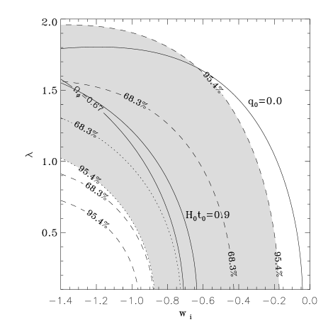
FIG. 8.: The 68.3% and 95.4% joint credible regions on the $w_{i}$ - $\lambda$ parameter space of the single exponential potential model, for the Sne IA test (dashed) and the gravitational lensing statistics test (dotted). Over plots are the contours of $H_{0}t_{0}=0.9$, $\Omega_{\phi 0}=0.67$, and $q_{0}=0$. The region allowed at 95.4% by both observational tests is shaded.

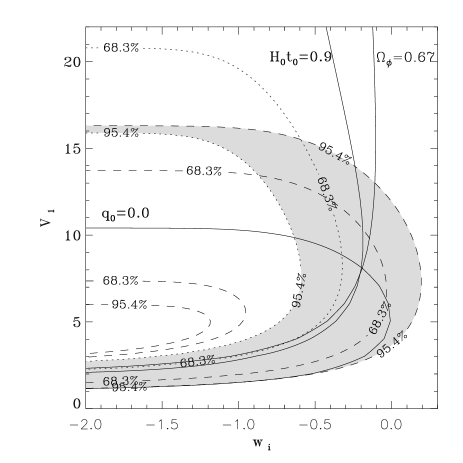
FIG. 9.: The 68.3% and 95.4% joint credible regions on the $w_{i}$ – $V_{1}$ parameter space of the double exponential potential model, for the Sne IA test (dashed) and the gravitational lensing statistics test (dotted). Over plots are the contours of $H_{0}t_{0}=0.9$, $\Omega_{\phi 0}=0.67$, and $q_{0}=0$. The region allowed at 95.4% by both observational tests is shaded.

V Discussion

We have performed a phase-space analysis on the double exponential potential model, its properties can be understood in terms of a single exponential potential model with a varying coefficient $\lambda$. The analysis shows that unlike the single exponential potential model which has two late times attractor depending on $\lambda$, the double exponential potential model has only one global attractor which leads to a matter dominated universe at late times. However, it is always possible for the model to be dominated by the scalar field at present and dominated by matter in the future. The problem with this model is we need to fine-tune the parameters in order not to have reached the attractor at the present epoch, thereby circumventing the objections of Binetruy [13] and de. la. Macorra [14]. However, all other quintessence models appear to also require a degree of fine-tuning [5, 6, 7, 8, 9, 10].

We studied the observation constraints for both the single and double exponential potential models using a more updated type IA supernovae data and the gravitational lensing statistics. The results show that there are regions in the parameter spaces for which the models are consistent with the observations at the same time giving appropriate values for the scalar field energy density and the age of the universe at present.

REFERENCES

- [1] Electronic address: cng@physics.adelaide.edu.au
- [2] R.R. Caldwell, R. Dave and P.J. Steinhardt, Phys. Rev. Lett. 80, 1582 (1998).
- [3] P. Steinhardt, in Critical Problems in Physics, ed. V.L. Fitch and D.R. Marlow (Princeton Univ. Press, 1997).
- [4] L. Wang, R.R. Caldwell, J.P. Ostriker, and P.J. Steinhardt, Astron. J. 530, 17 (2000).
- [5] C.T. Hill and G.G. Ross, Nucl. Phys. B311, 253 (1988); Phys. Lett. B203, 125 (1988); J.A. Frieman, C.T. Hill, A. Stebbins and I. Waga, Phys. Rev. Lett. 75, 2077 (1995).
- [6] P.J.E. Peebles and B. Ratra, Astrophys. J. 325, L17 (1988); Phys. Rev. D37, 3406 (1988); I. Zlatev, L. Wang and P.J. Steinhardt, Phys. Rev. Lett. 82, 896 (1999); Phys. Rev. 59, 123504 (1999).
- [7] C. Wetterich, Nucl. Phys. B302, 668 (1988); D. Wands, E.J. Copeland and A.R. Liddle, Ann. N.Y. Acad. Sci. 688, 647 (1993).
- [8] E.J. Copeland, A.R. Liddle and D. Wands, Phys. Rev. D57, 4686 (1998).
- [9] P.G. Ferreira and M. Joyce, Phys. Rev. D58, 023503 (1998).
- [10] A.R. Liddle and R.J. Scherrer, Phys. Rev. D59, 023509 (1999).
- [11] J.P. Deredinger, L.E. Ibanez, and H.P. Niles, Phys. Lett. B155, 65 (1985); M. Dine, R. Rohm, N. Seiberg, and E. Witten, Phys. Lett. B156, 55 (1985).
- [12] T. Barreiro, B. de Carlos, and E. J. Copeland, Phys. Rev. D58, 083513, (1998).
- [13] P. Binetruy, Phys. Rev. D60, 063502, (1999).
- [14] A. de la Macorra, hep-ph/9910330 (1999).
- [15] See S. Perlmutter et al., Astrophys. J. 517, 565 (1999), and references therein.
- [16] See A.G. Riess et al., Astron. J. 116, 1009 (1998), and references therein.
- [17] J.A. Frieman and I. Waga, Phys. Rev. D57, 4642 (1998).
- [18] P.S. Drell, T.J. Loredo and I. Wasserman, astro-ph/9905027 (1999).
- [19] C.S. Kochanek, Astrophys. J. 466, 638 (1996).
- [20] I. Waga and A.P.M.R. Miceli, Phys. Rev. D59, 103507 (1999).
- [21] I. Waga and J.A. Frieman, astro-ph/0001354 (2000).
- [22] S.C.C. Ng and D.L. Wiltshire, astro-ph/0004138 (2000).
- [23] A. de la Macorra and G. Piccinelli, hep-ph/9909459.
- [24] L.M. Krauss, astro-ph/9907308 (1999).