Infrared observations of gravitational lensing in Abell 2219 with CIRSI

Abstract

We present the first detection of a gravitational depletion signal at near-infrared wavelengths, based on deep panoramic images of the cluster Abell 2219 ($z$=0.22) taken with the Cambridge Infrared Survey Instrument (CIRSI) at the prime focus of the 4.2m William Herschel Telescope. Infrared studies of gravitational depletion offer a number of advantages over similar techniques applied at optical wavelengths, and can provide reliable total masses for intermediate redshift clusters. Using the maximum likelihood technique developed by Schneider, King & Erben (1999), we detect the gravitational depletion at the $3\sigma$ confidence level. By modeling the mass distribution as a singular isothermal sphere and ignoring the uncertainty in the unlensed number counts, we find an Einstein radius of $\theta_{\rm E}\simeq 13.7^{+3.9}_{-4.2}$ arcsec (66% confidence limit). This corresponds to a projected velocity dispersion of $\sigma_{v}\sim 800$ km s^-1, in agreement with constraints from strongly-lensed features. For a Navarro, Frenk and White mass model, the radial dependence observed indicates a best-fitting halo scale length of 125 h^-1 kpc. We investigate the uncertainties arising from the observed fluctuations in the unlensed number counts, and show that clustering is the dominant source of error. We extend the maximum likelihood method to include the effect of incompleteness, and discuss the prospects of further systematic studies of lensing in the near-infrared band.

1 Introduction

Gravitational lensing is now recognised as a valuable probe of the mass distribution in intermediate redshift ($z<0.4$) galaxy clusters independent of any assumptions about the nature of the lensing material (see reviews by Fort & Mellier 1995, Narayan & Bartelmann 1997, Mellier 1999, Bartelmann & Schneider 1999). For lenses at such redshifts, uncertainties arising from the redshift distribution of background sources are minimized and the angular scales of both weak and strongly-lensed features are well-suited for precise studies.

On small angular scales in super-critical systems, multiply-lensed arcs can provide useful absolute mass estimates provided spectroscopic redshifts and geometric constraints on the location of the various critical lines are available (e.g. Kneib et al. 1994, 1996). The most promising progress in constraining the mass on large scales has come from weak shear measurements (e.g. Fischer 1999; Hoekstra et al. 1998; Clowe et al. 1998) for which sophisticated inversion techniques have been developed (e.g. Kaiser & Squires 1993; Kaiser 1995).

However, cluster mass determinations based on weak shear signals are not without limitations. Firstly, the mass reconstruction from weak shear is non-trivial because of boundary effects due to the finite field of the data. To counter this effect, several finite-field methods have been proposed (e.g. Seitz & Schneider 1996). Secondly, since the shear arises from the gradient of the gravitational potential, the mass reconstruction is only known to within an additive constant. Accordingly, masses based on shear measurements are subject to a possible upward correction arising from a ‘mass sheet degeneracy’.

With sufficiently wide-field data it is possible to make the assumption that the surface mass density will approach zero at large distances from the cluster. However, with independent knowledge of the magnification of the lens, the mass-sheet degeneracy can be broken regardless of the field of view of the data. Two methods have been proposed to make use of this magnification information and calibrate the absolute scale of the mass distribution, either through the change of image size at fixed surface brightness (Bartelmann & Narayan 1995) or source counts (Broadhurst, Taylor & Peacock 1995).

This paper is concerned with exploring the role that infrared imaging offers in the gravitational depletion (or ‘convergence’) method for estimating the total masses of clusters. The depletion method was first suggested by Broadhurst, Taylor & Peacock (1995) who predicted the diminution in background galaxy surface number density as a function of radius expected behind a lensing cluster. Here we are concerned with extending the original test to near-infrared wavelengths where, in principle, there are significant advantages, namely the flatter number-count slope and a more accurate colour discrimination between foreground and background populations. The unique wide-field capabilities of the panoramic near-infrared Cambridge Infrared Survey Instrument (CIRSI, Beckett et al. 1998) allow us to test the method on the rich cluster Abell 2219 ($z$=0.22).

A plan of the paper follows. In $\S$2 we review the gravitational depletion method illustrating the difficulties associated with its implementation at optical wavelengths and the potential gains of repeating the experiment at near-infrared wavelengths. In $\S$3 we present new observations of Abell 2219 made at the prime focus of the 4.2m William Herschel telescope and discuss the techniques used to reduce the data as well as the methods used to create a sample of background galaxies. $\S$4 discusses the depletion signal observed in the context of various mass models and reviews the uncertainties involved. In $\S$5 we discuss the prospects of routinely estimating cluster masses using this method both with CIRSI and with the upcoming suite of wide field infrared survey telescopes.

2 Gravitational Depletion

The gravitational depletion or the ‘convergence’ method of breaking the mass-sheet degeneracy (Broadhurst, Taylor, & Peacock 1995) relies on the change in the surface number density of background galaxies induced by the magnification effect of a gravitational lens. Since only source counts are involved, exquisite image quality (essential for shear measurements) is not necessary. Furthermore, as the effect depends on the magnification $\mu$, absolute mass estimates are possible if the redshift distribution of the background sources is reasonably well-understood.

The intrinsic (unlensed) counts $n_{0}$ of galaxies brighter than some limiting magnitude $m$ are transformed to the observed (lensed) counts $n$ by

$$n(<m)=n_{0}(<m){\mu}^{2.5\alpha-1},$$ (1)

where $\alpha$ is the logarithmic slope of the number counts,

$$\alpha\equiv\frac{d\log n_{0}(m)}{dm}.$$ (2)

Two competing effects serve to change the lensed surface number density of the background galaxies. Source magnification clearly increases the surface number density by magnifying galaxies that would otherwise be fainter than the limiting magnitude. However, focusing within the beam dilutes the overall surface number density. The net effect depends on the value of $\alpha$: for $\alpha>0.4$ there will be an overall increase in observed surface number density, while for $\alpha<0.4$ a depletion is measured.

Unfortunately, at the limits where a sizeable fraction of field galaxies are expected to be behind an intermediate redshift cluster, the slope of the optical field counts, $\alpha\approx 0.4$, produces only a weak effect. In order to demonstrate the effect in one of the most massive clusters known, Abell 1689 ($z$=0.18), Taylor et al. (1998) restrict their analysis to a red subsample known a priori from blank field studies to have a flatter slope ($\alpha<0.4$). By colour-selecting sources redder than the sequence of cluster spheroidals, Taylor et al. simultaneously secure a background population whose $\alpha$ is sufficiently low for the depletion method to work, and with an unlensed surface number density of 12 arcmin^-2. Fort, Mellier & Dantel-Fort (1997) also search for an optical depletion effect behind the cluster CL0024+1654, by restricting their search to the magnitude ranges $26<B<28$ and $24<I<26.5$ where the slopes are found to be $\alpha_{\rm B}=0.17$ and $\alpha_{\rm I}=0.25$. However, they apply no colour selection to remove faint cluster members in this magnitude range, and furthermore are left with an extremely low number density of only a few galaxies per square arcmin. Similarly, Athreya et al. (in preparation) use photometric redshifts to isolate a background population for their weak lensing analysis of MS 1008-1224, but are hampered by a small field of view and background clustering. Clearly, balancing accurate discrimination of the lensing foreground from the background population while maintaining both a flat slope and sufficient numbers of background galaxies is of crucial importance, and it is for this reason that we turn to wide-field infrared observations.

Here we are concerned with extending the depletion method to near-infrared wavelengths, and we illustrate the possible advantages via an initial application to the rich cluster Abell 2219. The slope of the number counts flattens at longer wavelengths because of a reduced sensitivity to intermediate-redshift star forming galaxies (Ellis 1997). Moreover, this flattening occurs at progressively brighter apparent magnitudes. Without any colour selection, the slope of the counts at infrared wavelengths is sub-critical with $\alpha\sim 0.25$ at a relatively bright magnitude of $K\simeq 18$. This contrasts with optical counts which flatten only at very faint limits (e.g $\alpha\simeq 0.40$ for $V=22-24$ flattening to $\alpha=0.28$ beyond $V=24$ (Smail et al. 1995b)). Moreover, red-infrared colours (e.g. $I-K$) are more sensitive to redshift than to spectral class in the redshift range of interest. The opposite is true for say, $B-I$ (see Fig. 1). This leads to a much cleaner and efficient method of eliminating likely cluster members: we retain both the flat slope and sufficient numbers required for measurement of the depletion effect. The major drawback of measuring depletion signals in the near-infrared until now has been the absence of panoramic infrared detectors capable of surveying large areas of sky rapidly to the required depth. With the commissioning of the Cambridge Infrared Survey Instrument (CIRSI, Beckett et al. 1998), this becomes a practicality.

3 Data

3.1 Strategy

A number of factors enter when considering the merits of undertaking depletion studies at near-infrared wavelengths. Foremost, we can expect the counts to flatten considerably at cosmologically-significant depths for any passband longward of 1$\mu$m. Whereas classical number-count studies have been almost exclusively undertaken in the $K$- or $K^{\prime}$-band (e.g. Moustakas et al. 1997 obtain $\alpha=0.23$ for $18<K<23$; Gardner et al. 1993 obtain $\alpha=0.26$ for $K>18$), recent counts at $H$ (Yan et al. 1998) show little change in slope, with $\alpha=0.31\pm 0.02$ for $20<H<24.5$. Our lensing study will be undertaken using the $H$-band filter.

Secondly, in terms of colour-selection, the degeneracy between redshift and spectral class likewise improves dramatically when infrared magnitudes are added, particularly when account is taken of likely photometric errors. Fig. 1 illustrates a typical measurement of the $I-H$ and $B-I$ colour of a cluster early-type sequence at intermediate redshift. For the optical-optical colour we see that the single measurement is not enough to break the degeneracy between colour and redshift: an object bluer than the cluster sequence may be a low redshift elliptical or a late-type galaxy at any redshift. But when the optical-infrared colour is considered, the sensitivity to spectral type is greatly reduced, and we see that the bluer and redder galaxies map more cleanly onto foreground and background populations. One can therefore select more red objects with redshifts greater than that of the cluster. This accurate and efficient discrimination between the two populations is of great importance for our depletion study, which depends both on having a flat number count slope and a sufficient surface number density of background galaxies.

Our principal goal is to explore the depletion expected in Abell 2219 in the context of earlier studies of this cluster. This is an X-ray luminous (Allen et al. 1992) cluster lying at a redshift of 0.22, with an X-ray temperature of $T_{X}=11.8$ keV and showing no evidence of a cooling flow (Allen & Fabian 1998). The distribution of the X-ray gas is elliptical and misaligned with the cD galaxy on small scales. Smail et al. (1995a) report two systems of giant arcs with undetermined redshifts: a ‘red’ arc (possible two merging images of a single background source) and a ‘blue’ arc consisting of three separate segments. The red arc is shorter and brighter, and is prominent in our $H$-band image (Fig. 6).

Figure 1: Dependence of optical-infrared and optical-optical colour on redshift for early- and late-type galaxies derived from the GISSEL96 spectrophotometric codes (Bruzual & Charlot, in preparation) with and without evolution. The shaded area shows a range of colour when taking into account typical photometric errors of $\pm 0.2$ for the measurement of a typical early-type cluster sequence at intermediate redshift. Clearly the addition of the infrared magnitude reduces the dependence of colour on spectral type and allows for a more efficient selection of a background population. This is an obvious advantage over using optical colours alone to distinguish between foreground and background populations.

3.2 Observations

Table 1: Summary of observations

Pointing	$\alpha$ (J2000)	$\delta$ (J2000)	total exposure time	seeing
CIRSI $H$-band, cluster centre	16 40 20.5	46 42 44.8	5.3 h	0.9″
CIRSI $H$-band, offset fields	16 39 50.2	46 42 44.8	5.5 h	0.9″
$I$-band EEV	16 40 20.5	46 42 44.8	1.0 h	0.8″

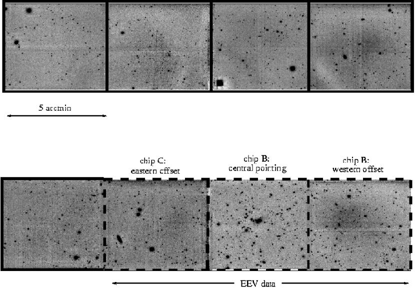
Figure 2: The field of view of CIRSI after two adjacent pointings. The resulting two strips each measure $\sim 20\times 5$ arcmin. The dashed lines indicate the region which overlapped with the optical data. Treating the individual CIRSI chips as separate images, the western offset field, central cluster field, and eastern offset field (all with overlapping optical data) are labelled. North is up, east is to the left.

The Cambridge Infrared Survey Instrument (CIRSI, Beckett et al. 1998) is a wide-field infrared imager consisting of a mosaic of four 1K $\times$ 1K Rockwell Hawaii HgCdTe detectors. Each detector is separated by a gap of approximately one detector width so that multiple pointings can be easily arranged to produce a larger contiguously-imaged field.

Table 1 summarizes the observations that form the basis of this paper. The $H$-band CIRSI observations of Abell 2219 were made at the prime focus of the 4.2-m William Herschel Telescope (WHT); this offers a plate scale of 0.32 arcsec pixel^-1. Each CIRSI detector has a field of view of $5.5\times 5.5$ arcmin so the mosaic of four detectors gives an instantaneous total field of view of $11\times 11$ arcmin.

The cluster was observed on the nights 1 to 4 July 1999 using a field configuration chosen to optimally overlap with existing $B$- and $I$-band EEV CCD data of plate scale 0.24 arcsec pixel^-1. Two adjacent CIRSI pointings were arranged to ensure two contiguous strips of approximately $5\times 20$ arcmin each, one of which overlaps the two-pointing 16 $\times$ 16 arcmin EEV field (Fig. 2).

The optical CCD data were taken as part of a companion programme and its reduction is discussed elsewhere (Bézecourt et al., 2000). The CIRSI observations were taken using short (30 sec) exposures with a 9 point pattern dithered with an offset of 15 arcsec. Larger offsets of the order of 50 arcsec were made before starting a new dither sequence. Typically 10 exposures were taken at each position, and the first exposure in each sequence was processed separately due to instability in the large scale bias level.

Data reduction was done using routines from the CIRSI data reduction pipeline cirdr (Chan et al. 1999, Hoenig et al. 1999) in iraf. For each dither sequence, a median sky image was created. The sky image was then scaled to and subtracted from each of the individual science images. The objects were located and a mask for each frame was constructed using routines from Pat Hall’s phiirs infrared data reduction package (Hall, Green & Cohen 1998). The original images were medianed a second time using the object masks to prevent contamination, and this second-pass sky was again subtracted from each of the science images.

The resulting sky-subtracted images were averaged using integer pixel offsets and a 3-sigma clipping rejection algorithm was applied. To construct the final image, the combined dither sequences from each night’s observing were averaged in the same manner. Finally, the noisier regions at the edge of each mosaic where the overlap of dither sequences was incomplete were trimmed. Treating each detector as a separate image, one dither sequence was calibrated using measurements of a standard star from the UKIRT NIR catalogue (Hawarden et al. , in preparation). A set of secondary standards within the science image were then measured and used to calibrate the final mosaiced image, taking care to consider possible discrepancies in the overlap regions between the chips.

We used SExtractor 2.0 (Bertin & Arnouts 1996) to detect sources and perform isophotal photometry, selecting a detection and analysis threshold of 1.5$\sigma$ above the sky background. The $H$-band images were registered to the $I$-band data and SExtractor was run in double image mode. This allowed us to detect the objects in the $I$-band and measure both magnitudes with the same isophote. The catalogues were visually inspected and spurious sources removed.

Fig. 2 shows the final reduced $H$-band image and indicates the degree of overlap with the EEV CCD data of Bézecourt et al. (2000).

3.3 Completeness and Contamination

To understand the magnitude limit of our $H$-band data, we performed simulations by creating noise-only images: we randomized the offsets and thus created a misaligned mosaic with the same dimensions and noise properties as the science images, but with all the objects removed. We added artificial galaxies of known magnitudes to these images using the artdata package in IRAF and recovered them using SExtractor. We found that for a detection in the $H$-band, the 50% completeness level (the magnitude at which Sextractor recovered 50% of the input galaxies) agreed well with the turnover in the observed number counts at $H=21.7$. However, for purposes of measuring colour, we made the detections in the $I$-band and so were able to push the infrared magnitude limit even deeper. Fig. 3 shows our resulting $H$-band number counts compared to previous infrared surveys.

Figure 3: Comparison of the CIRSI $H$-band number counts with those from the literature. Shown are the two CIRSI offset fields (covering 27 arcmin² each), the Yan et al. (1998) $H$-band survey, and the Gardner et al. (1993) and Moustakas et al. (1997) $K$-band surveys. For comparison purposes the $K$-band points have been shifted by one magnitude according to the approximation $H-K=1$. The counts from the literature have all been corrected for incompleteness at faint magnitudes.

In addition to adopting a strictly IR-limited sample, we have also explored alternative detection strategies noting that we seek the relative depletion in the counts as a function of position, i.e. uniformity of detection is more important than completeness. We show in Appendix A that, for the purposes of our depletion measurements, it is not necessary to have a complete catalogue, so long as the incompleteness function responsible for the observed fall-off from the intrinsic power-law distribution is the same for the offset fields as for the lensed fields. As we determined the offset counts simultaneously under identical observing conditions, this holds true for our sample. We therefore push the limits of the $H$-band catalogue past the completeness threshold and adopt a working limit of $H=24$ for our sample, so that it remains $H$-limited.

As discussed in Appendix A, it is important to consider not only the completeness of the sample but also its contamination by spurious sources arising from noise peaks, especially when the counts are extended past the completeness limit. If we define the noise fraction as the fraction of false objects per magnitude bin, we may proceed with an incomplete sample only if the noise fraction brighter than our limiting magnitude is small. To estimate this we used the same pure noise image discussed above, and measured the magnitudes in 500 randomly placed apertures. Table 2 shows the resulting distribution of magnitudes, with only 3.6% of ‘detections’ falling below the $H=24$ cutoff. This should be considered as an upper limit, since the detection in our sample is performed in the deeper $I$-band image. Moreover, contamination, if it is left unaccounted for, will tend to reduce the lensing signal. We therefore conservatively ignore this small effect in our analysis.

magnitude range	number of objects	fraction
$23<H<24$	18	3.6%
$24<H<30$	235	47.0%
$H=$INDEF	247	49.4%

Table 2: Noise fraction for the $H$-band image. Magnitudes were measured in 500 randomly placed apertures on a pure noise $H$-band image. The results show that the number of false objects brighter than our magnitude limit of $H=24$ is negligible.

3.4 Removal of Cluster Members

An essential precursor in examining a possible depletion effect in Abell 2219 is the location of the lensing and unlensed population of galaxies, the latter of which is, of course, dominated for such a low redshift system by cluster members. The sequence of cluster galaxies is clearly visible on the $I-H$ colour magnitude diagram shown in Fig. 4. Taking into account known members and photometric errors, cluster galaxies can be optimally excised according to the relation

$$\left|I-H-(3.266-0.0865H)\right|<0.2.$$

Figure 4: Colour-magnitude diagram for all objects in the cluster field. The cluster galaxies are indicated by filled circles; the population of objects selected for lensing purposes are those with colours redder than the cluster sequence and with $18<H<24$ (dashed line).

We can divide the remaining population of field galaxies into ‘red’ and ‘blue’ (unlensed) field populations, adding the further constraint that $18<H<24$ and noting that the blue population could be composed of both foreground and blue cluster members.

The two CIRSI chips on either side of the central cluster pointing provide us with flanking fields to characterize the field population. Combining the catalogues for the east and west flanking fields, we apply the same colour-selection to determine the properties of the unlensed background population. Fig. 5 shows the resulting number counts for the sub-populations, which are described by

$$\log N_{red}=(0.185\pm 0.017)H+(0.23\pm 0.35),$$

and

$$\log N_{blue}=(0.222\pm 0.030)H+(-0.89\pm 0.61).$$

for the range $19<H<22$ that is well described by a power-law distribution. Up to $H=24$, the number densities of the background populations are $n_{0}=20.3$ and $n_{0}=10.5$ arcmin^-2 for the red and blue populations, respectively.

Figure 5: Number-magnitude relation for non-cluster galaxies in the offset fields. Open circles are galaxies redder than the cluster sequence; filled circles are objects bluer than the cluster sequence. Note that the slope of the counts for the blue population is not significantly steeper than that of the red population (as is seen in the optical, e.g. Taylor et al. (1998)). Nevertheless we consider only the red objects for lensing purposes in order to minimize contamination by foreground galaxies.

Finally, to account for obscuration of background galaxies by foreground cluster members, we created a mask image using the SExtractor ‘segmentation’ option. This assigns each pixel in the image a value according to the object that contains it. We then used the location of the cluster galaxies (as well as those few non-cluster objects with $H<18$) selected above to extract those pixels and form a mask which we used in the subsequent depletion analysis.

4 Results

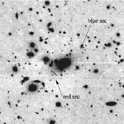
Figure 6: The central $2.7\times 2.7$ arcmin of the $H$-band CIRSI image, showing the red arc reported in Smail et al. (1995a). The second, bluer arc system is only barely visible in this infrared image.

Our plan will be first to demonstrate the existence of the IR depletion behind Abell 2219 using the $I-H$ colour diagram to isolate cluster members and select a background population ($\S$3.4). We will then attempt to quantify the effect by employing maximum likelihood methods to fit simple, one-parameter models to the mass distribution for the cluster. Finally, we will consider the effect of uncertainties in the adopted mean surface number density on the maximum likelihood results.

4.1 Depletion Analysis

Fig. 7 shows the radial density profile for field galaxies selected as discussed in $\S$3.4, taking into account the area masked by the colour-selected cluster galaxies (3.0 arcmin² in total out of the 27.5 arcmin² central field). We utilize both flanking fields in order to determine the unlensed surface number density of the red population to be $n_{0}$=20.3 arcmin^-2. With no colour selection this density rises to $n_{T}$=43.2 arcmin^-2 which gives some indication of the likelihood that non-cluster galaxies might be discarded via this colour cut.

Fig. 7 gives a clear detection of the depletion signal at the 3$\sigma$ level within a diameter of $\sim$80 arcsec ($\sim$350 kpc for $h=0.5$, $q_{o}=0.5$). However, its absolute significance depends critically on the adopted value of $n_{0}$. We estimate the uncertainty in our measurement of $n_{0}$ (indicated by the dashed lines in Fig. 7) using the dispersion in counts in the full $H$-band dataset shown in Fig. 2. The effects of this uncertainty are discussed further in $\S\ref{sec-err}$.

Figure 7: Ratio of observed number density to unlensed number density of red galaxies with distance from the cluster centre, using a bin width of 14 arcsec. All measurements take into account the area in each bin obscured by the cluster galaxies. A depletion of number counts is clearly seen at small radii. The dashed lines indicate the errors in the measured value of $n_{0}$, the unlensed number density (the effect of this uncertainty is considered in Section $\S\ref{sec-err}$). The thick line shows the expected depletion profile induced by a SIS with $\sigma_{v}\sim 800$ km s^-1.

To investigate the magnitude and significance of this possible depletion, we adopted a maximum likelihood approach based on that developed by Schneider, King & Erben (2000; hereafter SKE). In this formulation, which avoids the loss of information induced by the radial binning (as in Fig. 7), the log-likelihood equation takes the form:

$$l=-n_{0}\int d^{2}\theta[\mu({\mathbf{\theta})}]^{2.5\alpha-1}+(2.5\alpha-1)\sum_{i=1}^{N}\ln\mu({\mathbf{\theta}}_{i}),$$ (3)

where $n_{0}$ is the unlensed number density of background galaxies (arcmin^-2), $\mu$ is the magnification, ${\mathbf{\theta}}_{i}$ is the position vector of the $i$th galaxy in the field with respect to the cluster centre, $N$ is the total number of galaxies observed, and $\alpha=d\log{N}/dm$ is the intrinsic logarithmic slope of the number counts. The first term in the log-likelihood function addresses the probability of finding $N$ galaxies in the field of view given the lens model $\mu(\theta)$ and the population parameters $\alpha$ and $n_{0}$, while the second term concerns the probability of finding each galaxy $i$ at position $\theta_{i}$. By maximizing $l$ we find the most likely parameter(s) for a given lens model. In the subsequent sections, we examine two single-parameter mass models.

The derivation of this expression is presented in Appendix A. Importantly, this appendix also generalizes the likelihood method of SKE to include the effect of incompleteness. We showed that, as long as the intrinsic unlensed counts follow a power law, incompleteness is very simple to account for: one simply uses the observed (incomplete) unlensed density $\tilde{n}_{0}$ in place of the intrinsic (complete) unlensed density $n_{0}$ in the likelihood function. This allows us to include, in our sample, galaxies which are fainter than the completeness limit and therefore of improving our signal-to-noise, without fear of introducing a bias.

4.1.1 Model 1: Singular isothermal sphere

First, we model the cluster according to a singular isothermal sphere (SIS) parametrized with the Einstein radius, $\theta_{\rm E}$:

$$\mu_{\rm SIS}(\theta)=\left|\frac{1}{1-\theta_{\rm E}/\theta}\right|.$$ (4)

The filled circles in Fig. 8 show the resulting log-likelihood curve. The sharp dips are a result of the contribution of the second term of Equation 3 (concerning the galaxy positions) to the log-likelihood function. As the likelihood is calculated for increasing values of the input $\theta_{E}$, a galaxy may happen to lie on the critical line ($\theta_{i}=\theta_{E}$). Since the magnification (and hence the depletion) is formally infinite at this radius, the probability of finding a galaxy vanishes, and the method rejects this particular model. This results from the fact that we have effectively modelled the galaxies as point sources. In practice, galaxies are extended objects and therefore are not subject to infinite magnifications, but instead are stretched into giant arcs on the critical line. In our analysis, we simply identified the peak as the absolute maximum, without any interpolation. As we will see below, this does not introduce any observable bias in the determination of the model parameters.

The peak of the likelihood function is reached at $\hat{\theta}_{\rm E}=13.7$ arcsec, which is consistent with the location of the red giant arc located 13 arcsec from the cluster centre (shown in Fig. 6).

Figure 8: Maximum likelihood analysis for depletion of the red background galaxy sample (solid circles). The model corresponding to the peak is a SIS parametrized by the Einstein radius $\hat{\theta}_{E}=13.7$ arcsec. By contrast, the same analysis for the red galaxy sample in one of the offset fields (open circles) peaks at $\hat{\theta}_{E}=0$ arcsec and shows no evidence of depletion, as does the sample of blue (foreground) galaxies in the cluster field (open triangles). The curves have been vertically shifted to the same zeropoint for clarity.

We perform a test of the depletion by applying the same maximum-likelihood test on one of the offset fields. Using the same colour selection criteria to define a population of red objects we find no evidence for any depletion effect. Furthermore, we also test the population of ‘foreground’ galaxies (those with colours bluer than the cluster sequence) in the cluster field, and again find as expected no evidence for depletion. The log-likelihood functions for these two samples, both peaking at $\theta_{E}=0$ arcsec, are also shown as open symbols in Fig. 8.

4.1.2 Model 2: The NFW profile

An alternative model to the SIS is the universal density profile for dark matter halos proposed by Navarro, Frenk & White (1997, 1996, 1995). Given the uncertainties in the data it is unlikely that we could use this technique to distinguish between two models. It is nevertheless of interest to demonstrate how the method could be applied to a second model.

The NFW density profile follows

$$\rho(r)=\frac{\delta_{c}\rho_{c}}{(r/r_{s})(1+r/r_{s})^{2}},$$ (5)

where $\rho_{c}$ is the critical density at the redshift of the lens. The two parameters of the model are contained in the scale radius $r_{s}$ and the concentration parameter $c$, so that the characteristic overdensity is

$$\delta_{c}=\frac{200}{3}\frac{c^{3}}{\ln(1+c)-c/(1+c).}$$ (6)

In contrast to the SIS, this profile flattens towards the core and is capable of producing radial as well as tangential arcs (Bartelmann 1996). For a projected radial distance $R$, we can define a dimensionless distance, $x=R/r_{s}$. Wright & Brainerd (1999) give the formulation for the radial dependence of the surface density $\Sigma(x)$ and the shear $\gamma(x)$. The convergence is then simply $\kappa(x)=\Sigma(x)/\Sigma_{\rm crit}$, where the critical surface number mass density

$$\Sigma_{c}=\frac{v_{c}^{2}}{4\pi G}\frac{D_{s}}{D_{d}D_{ds}}$$ (7)

depends on the angular diameter distances $D_{s},D_{d},D_{ds}$ from observer to source, observer to lens, and source to lens, respectively, and the speed of light $v_{c}$. The magnification is then simply

$$\mu_{\rm NFW}(x)=\left|\frac{1}{(1-\kappa(x))^{2}-\gamma(x)^{2})}\right|,$$ (8)

(e.g. Schneider, Ehlers and Falco 1992).

Using $\mu_{\rm NFW}$ in Equation 3, we perform the maximum likelihood analysis for an NFW profile on Abell 2219. We reduce the model to one parameter by assuming a reasonable value for the concentration parameter, namely $c=6$, and fitting for $r_{s}$. We find a maximum at $r_{s}$ corresponding to an angular length of 52 arcsec. At the redshift of the cluster this gives a scale length of 125$h^{-1}$ kpc (where $H_{0}=100h$ km s^-1 Mpc^-1), which compares well to the $r_{s}\sim 250h^{-1}$ predicted from numerical simulations of CDM models (Bartelmann 1996).

Fig. 9 shows the form of an NFW depletion curve resulting from the substitution of $\mu_{\rm NFW}$ in Equation 1, for such a cluster with $c=6$ and $r_{s}=125h^{-1}$ kpc . The observed depletion curve of Abell 2219 is overplotted for comparison, and we see that the data are also consistent with this model. However, the data do not allow us to distinguish between the NFW and SIS models. In the further analysis we choose to continue with the SIS for simplicity.

Figure 9: The radial depletion curve for a NFW cluster with $r_{s}=125h^{-1}$ kpc and $c=6$. The inner dip corresponds to the radial arc at $x_{r}=2$ arcsec while the outer dip corresponds to the tangential arc at $x_{t}=5$ arcsec, for a source population with $\alpha=0.185$. Overlayed are the points the Abell 2219 depletion curve, as in Fig. 7.

4.2 Simulations

To further test the robustness of the depletion effect we have simulated a population of galaxies with the same properties as our putative background population. In our observed sample the intrinsic power law form of the background number counts is modified by the incompleteness function. As shown in Appendix A, it is however equivalent to use a renormalized power law for the counts in the simulations. Specifically, we keep the same observed slope, $\alpha=0.185$ but lower the normalization to maintain the same observed unlensed number density $\tilde{n}_{o}=20.3$ arcmin^-2.

Scattering the simulated galaxies randomly across the field of view, we then adjusted their positions and magnitudes as if they were lensed by a singular isothermal sphere with $\theta_{\rm E}=13.7$ arcsec. We created a catalogue of those galaxies whose lensed magnitudes were brighter than our limiting magnitude and whose lensed positions were not obscured by the Abell 2219 cluster mask and applied the same maximum likelihood technique. Fig. 10 shows the distribution of the resulting best-fitting models for 200 realizations. We see that the distribution of recovered Einstein radii is centred around the input value of 13.7 arcsec, and deduce the 95% confidence interval to span the range $6.8<\hat{\theta}_{E}<26.5$ arcsec.

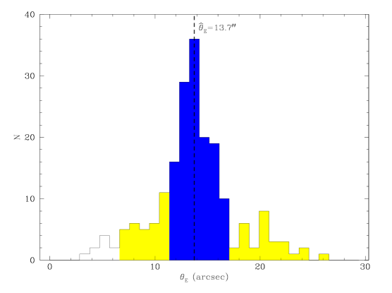
Figure 10: Distribution of the recovered $\theta_{\rm E}$ from 200 realizations of simulated lensing by an isothermal sphere, using the observed background population parameters ($n_{0}=20.3$ arcmin^-2, $\alpha=0.185$). The darker shaded region indicates the resulting 66% confidence interval in the range $11.1<{\theta}_{E}<17.06$ arcsec, centred around the input value of $\hat{\theta}_{\rm E}=13.7$ arcsec. The lighter shaded region indicates the 95% confidence interval in the range $6.8<{\theta}_{E}<26.5$ arcsec.

To translate the estimates of $\theta_{\rm E}$ into an statement regarding the cluster mass, we use the relation for a SIS:

$$\theta_{\rm E}=4\pi\frac{\sigma^{2}_{v}}{c^{2}}\frac{D_{\rm ds}}{D_{\rm s}},$$ (9)

where $\sigma^{2}_{v}$ is the velocity dispersion of the lens, $D_{\rm ds}$ and $D_{\rm s}$ are the angular-diameter distances from lens to source and from observer to source, respectively.

Modelling the background $N(z)$ from the $K$-band surveys of Cowie et al. (1996), we find the median redshift for the background is $\left<z\right>=1.0$ for $H<22$, increasing to $\left<z\right>=1.3$ at $H<24$. Given $z_{\rm lens}=0.22$ and assuming a cosmology of {$H_{0}=50$ km s ^-1 Mpc ^-1, $q_{o}=0.5$} we obtain $\sigma_{v}=842^{+112}_{-141}$ km s^-1 for $\left<z\right>=1$ and $\sigma_{v}=814^{+109}_{-136}$ km $s^{-1}$ for $\left<z\right>=1.3$. The quoted errors refer to the 66% confidence limits derived from the above simulations. Clearly the result is more sensitive to the uncertainties in the measurement of $\theta_{E}$ than the uncertainties in the background redshift distribution. Therefore, we consider the background to lie on a single sheet at the median redshift, and placing the galaxies at $z=1.3$ and adding the errors in quadrature we obtain our final result of $\sigma_{v}=814^{+112}_{-139}$ km s^-1 (66% confidence level). Our SIS model is in good agreement with the result from Smail et al. (1995a), who find $\sigma_{v}\sim 930$ km s^-1 using strong lensing constraints. Note that the precision of the strong lensing constraint would be tighted if the redshift of the red arc were known. Our results are also consistent with the optical weak shear analysis of Bézecourt et al. (2000), who find $\sigma_{v}=1075\pm 100$ km s^-1 from an optical weak shear analysis. In principle, by adding one additional parameter to our model we could also constrain the amplitude of a mass-sheet, and therefore break the degeneracy inherent in reconstructions involving shear only. However, fitting an extra parameter is not warranted by the data, especially after taking into account the uncertainty in $n_{0}$ (see §4.3 below).

The above simulations only enable us to deduce the error on $\theta_{E}$ assuming our initial estimate of the model parameters is correct. To test the method across a wider range of input lenses, we have simulated lenses with input parameters $\theta_{\rm E}=0,10,20,$ and 30 arcsec, and performed the maximum likelihood analysis 25 times in each case. Fig. 11 shows the recovered $\hat{\theta}_{\rm E}$ vs the input $\theta_{\rm E}$, both with and without the cluster mask. We see that neither the dips in the likelihood function, nor the masked area introduce any significant bias into the method. In addition, we find that obtaining a best-fitting value of $13.7$ in the absence of lensing, i.e. a false detection, is unlikely, and we reject this null hypothesis at the 6$\sigma$ level. This figure provides a measure of the significance of our detection of the lensing signal if the uncertainty in $n_{0}$ is ignored and the assumed model is correct.

Figure 11: Simulations showing recovered $\theta_{E}$ vs input $\theta_{E}$, with and without a cluster mask (the open circles are offset slightly in the $+x$ direction for clarity). The cluster mask, which obscures about 10% of the field including much of the central region, has no significant effect on the recovered $\theta_{E}$ (aside from increasing the errors), even given the low numbers of background galaxies.

4.3 Effect of uncertainty in number counts

SKE demonstrate that, to first order, most of the magnification information is provided by the unlensed number density $n_{0}$. Without adequate knowledge of this normalization, the mass-sheet degeneracy cannot be broken. Prior knowledge of the uncertainty in $n_{0}$ can be included in the maximum-likelihood analysis. Assuming that the true $n_{0}$ follows a Gaussian distribution with mean $\bar{n}_{o}$ and dispersion $\sigma_{n}=\eta\bar{n}_{o}$ then, as shown in SKE, the log-likelihood function becomes:

$$l(\eta)=-n_{0}I+(\beta-1)\sum_{i=1}^{N}\ln\mu({\mathbf{\theta}}_{i})+N\ln n_{0}-\left(\frac{(n_{0}-\bar{n}_{o})^{2}}{2\left(\eta\bar{n}_{o}\right)^{2}}\right),$$ (10)

where $I=\int d^{2}\theta[\mu({\mathbf{\theta})}]^{\beta-1}$ and $\beta=2.5\alpha$. This can be maximized with respect to $n_{0}$, yielding

$$\frac{n_{0}}{\bar{n}_{o}}=\frac{1}{2}\left(1-\eta^{2}\bar{n}_{o}I\right)+\sqrt{\frac{1}{4}\left(1-\eta^{2}\bar{n}_{o}I\right)+\eta^{2}N}.$$ (11)

Substituting this value for $n_{0}$ into Equation 10 yields the new log-likelihood function.

To determine the value of $\eta$ for our own sample, we turn to the entire $H$-band dataset pictured in Fig. 2. While the sample used in the depletion analysis is a colour-selected sample that incorporates the $I$-band data, the area in common with the optical image allowed for only the two offset fields discussed previously. However, we attempt to estimate the uncertainty in $n_{0}$ by sampling the counts in the entire $H$-band region.

We divided the two $H$-band strips into four single-chip images each, discarding the chip containing the cluster and the two images taken with chip 3 (which was contaminated by many hot pixels, leading to a high number of false detections). This left five offset images of equal area. We constructed $H$-limited catalogues on the central $4.3\times 4.3$ arcmin region of each image using SExtractor and examined the dispersion in the total $H$-band number counts in the range $18<H<24$ for each chip. The resulting distribution of raw counts, listed in Table 3, has mean $\bar{N}=467$ and standard deviation $\sigma=40$, hence the fractional error is $\eta_{\rm H}=0.086$. If the fraction of galaxies discarded during the colour selection to form the ‘red’ sample of background galaxies is constant from field to field (from the two multi-colour offset fields it appears to be $\sim 50\%$), then this error will also apply to the subpopulation.

field	N($18<H<24$)
1	468
2	516
3	483
4	476
5	394

Table 3: $H$-band counts in 18.2 arcmin² regions in five of the seven offset fields, yielding a fractional uncertainty of 8.6%.

We note that this is higher than the Poisson error for these number counts. However, if we consider the angular correlation function $\omega(\theta)$ of $K$-band galaxies to $K=21.5$ presented in Carlberg et al. (1997) and extrapolate to $\theta=2.5$ arcmin then $\omega(\theta)\sim 0.01$. This yields a rough estimate of $\delta N/N\sim\sqrt{\omega(2.5^{\prime})}\sim 0.1$ which is in agreement with our measurement of the dispersion. Our uncertainty in the unlensed density is therefore dominated by clustering.

We again turn to simulations to derive the error bars on our measurement. As in $\S\ref{sec-sim}$ we simulate a population that is lensed by a SIS with $\theta_{E}=13.7$ arcsec, but in this case we draw the true value of $n_{0}$ from a Gaussian distribution with mean 20.3 arcmin² and dispersion $\sigma_{n}=\eta n_{0}$, where $\eta=0.086$ as derived above. Using the log-likelihood function in Equation 10 and a fixed estimate $n_{0}=20.3$, we show the resulting distribution of recovered $\theta_{E}$ for 200 realizations in Fig. 12. We see, by comparison with Fig. 10 (the case where $n_{0}$ was known precisely), that incorporating an error of $\eta=0.086$ produces a much broader distribution, with the result of greatly increasing the error bars on our measurement. Applying Equation 10 to the real data, we find $\hat{\theta}_{E}=1.4^{+5.2}_{-1.4}$ arcsec (66% confidence) or $\hat{\theta}_{E}=1.4^{+15.9}_{-1.4}$ (95% confidence). While the estimate of $\theta_{E}$ itself is greatly reduced, the error bars make it compatible with the result of $\S\ref{sec-sim}$ within a 2$\sigma$ range.

This section illustrates the principal weakness of the depletion method as pointed out in SKE, namely the vital importance of accurately measuring $n_{0}$. With a $\delta N/N\sim 0.1$ which is not unreasonable given clustering on these scales, the depletion effect is made more difficult to distinguish from variations in the background counts that are not due to lensing. However, this effect could be countered by selecting similar clusters (e.g. by their X-ray temperatures) and stacking the depletion signal accordingly, thus calibrating the cluster $T_{X}$-mass relation and obtaining an average cluster mass profile. Choosing a sample of 10 clusters would simultaneously increase the effective background surface number density by a factor of 10 while reducing the fractional error in $n_{0}$ by a factor of $\sqrt{10}$. Simulations show that for 10 clusters similar to Abell 2219, the 95% confidence region on $\theta_{E}=13.7$ arcsec would then shrink from $0.9<\theta_{E}<29.6$ arcsec (as quoted above) to only $7.7<\theta_{E}<16.1$ arcsec; a feasible project for upcoming IR survey telescopes. Note that in practice scatter in the cluster properties would increase this range somewhat.

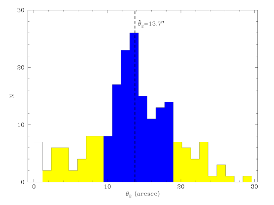
Figure 12: The effect of uncertainty in the background number counts from simulations. Shown is the distribution of the recovered $\theta_{E}$ for 200 realizations, with the true $n_{0}$ drawn from a Gaussian distribution with mean 20.3 arcmin^-2 and fractional error $\eta=8.6$%. The lensed populations were analysed as in Equations 10 and 11 using the estimated $\bar{n}_{o}$=20.3 arcmin^-2. The 66% and 95% confidence limits are indicated by the dark ($8.9<{\theta}_{E}<18.9$) and light ($0.9<{\theta}_{E}<29.6$) shaded regions. A comparison with Fig. 10 shows that incorporating a significant uncertainty in the analysis increases the error bars on the measurement of $\theta_{E}$.

5 Conclusions

We present a study of the depletion effect around Abell 2219, the first done in the infrared, using the newly-available panoramic IR camera (CIRSI). We show (see Appendix A) that the sample can be effectively exploited beyond the completeness limit, as long as the lensed field and the background field obey the same incompleteness functions and have minimal contamination by false objects. This allows us to detect a clear dip in the radial number density profile of background galaxies at small distances from the cluster centre. The optical-infrared colours enable us to select a population of red background galaxies with a flat number-count slope in order to optimise the lensing signal and reduce foreground-background confusion.

For a population of red background galaxies with an extremely flat slope ($\alpha=0.185$), we employ maximum likelihood methods and a SIS model to derive an estimate of the Einstein radius $\theta_{E}=13.7^{+3.9}_{-4.2}$ arcsec (66% confidence limit when uncertainties is $n_{0}$ are ignored), resulting velocity dispersion $\sigma_{v}=814^{+112}_{-139}$ km s^-1. These values are consistent with the location of the redder of the two giant arcs and the estimate $\sigma_{v}\sim 930$ km s^-1 of Smail et al. (1995a).

We examine the uncertainty in the number counts, and derive a fractional error of 8.6% on the normalisation of the background number density (consistent with clustering on these scales). When this error is incorporated into the maximum-likelihood analysis the error bars become too large to make a precise statement about the magnitude of the lensing (although our previous measurement is not ruled out). This demonstrates the crucial importance of the background density $n_{0}$ for an accurate depletion analysis as discussed in Schneider, King & Erben (2000).

Finally, while we cannot at present use our current data to distinguish between alternative models for the cluster mass distribution, we demonstrate the application of the method to the data using a second mass model. We show the typical depletion curve induced by a cluster with an NFW density profile, and using this profile as a second estimate of the cluster mass we derive a scale length of 125$h^{-1}$ kpc for the cluster.

The wide field IR coverage available using CIRSI is an ideal match to the current generation of wide-field optical imagers. The availability of multicolour data taken simultaneously but at large radii from the cluster centre provides offset information about the field population and eliminates the need to normalise the depletion curve to the values at the edge of the chip, and the infrared sample provides a cleaner discriminant between foreground and background and a flat number-count slope.

The depletion method is an elegant and relatively simple way to derive mass estimates of clusters of galaxies. Deeper IR surveys will provide more accurate knowledge of $\omega(\theta)$ on arcminute scales, allowing us to better understand the degree to which clustering affects the method. Future studies of clusters with wide-field optical-infrared data (e.g. with the VISTA telescope, http://www-star.qmw.ac.uk/$\sim$jpe/vista) covering a wide wavelength range could provide more accurately selected background populations via photometric redshifts and allow us to add another sample of independent mass profiles to be compared with those derived from velocity dispersions, X-ray measurements, and strong and weak lensing. The problem posed by the uncertainty in the background number counts can be overcome by selecting similar clusters (e.g. by their X-ray temperatures) and stacking the depletion signal accordingly to obtain an average cluster mass profile; a feasible project for future IR survey telescopes.

Appendix A Effect of Incompleteness

The likelihood function for the lensing depletion has been derived by SKE, for the case of a complete sample of background galaxies. Here we generalize their results to include the effect of incompleteness in the sample.

Let the unlensed differential counts of the background galaxies be denoted by $\frac{dn_{0}(S)}{dS}$, where $n_{0}$ is the number of galaxies per unit solid angle, and $S$ is the flux. The lensed counts are given by

$$\frac{dn(S)}{dS}=\frac{1}{\mu^{2}}\frac{dn_{0}(\frac{S}{\mu})}{dS},$$ (12)

where $\mu$ is the magnification. The observed (lensed) counts, in the presence of incompleteness, can be written as

$$\frac{d\tilde{n}(S)}{dS}=\frac{dn(S)}{dS}\phi(S),$$ (13)

where $\phi(S)$ is the completeness fraction for a given flux $S$. Typically, $\phi=1$ for large fluxes, and $\phi<1$ for small fluxes. In the following, we will continue to use the subscript ₀ to denote unlensed counts, and a tilde to denote the observed counts. In practice, it is convenient to consider the total counts down to a detection limit $S$

$$n(>S)=\int_{S}^{\infty}dS^{\prime}\frac{dn(S^{\prime})}{dS}.$$ (14)

In our case (see Fig. 5) and for many applications, the intrinsic unlensed counts are well described by a power law of the form

$$\frac{dn_{0}}{dS}\propto S^{-\beta-1},~{}~{}~{}n_{0}(>S)\propto S^{-\beta},$$ (15)

where $\beta$ is the flux slope parameter, which is related to the magnitude slope parameter $\alpha\equiv d(\log n_{0})/dm$ (Equation 2) by $\beta=2.5\alpha$. In this case, Equation (12) takes the simple form

$$n(>S)\left/n_{0}(>S)\right.=\frac{dn}{dS}\left/\frac{dn_{0}}{dS}\right.=\mu^{\beta-1}.$$ (16)

In this case, the observed lensed counts are given by

$$\frac{d\tilde{n}}{dS}=\phi\mu^{\beta-1}\frac{dn_{0}}{dS}.$$ (17)

As a result, the mean integrated lensed counts $\langle\widetilde{N}\rangle$ observed in the field are given by

$$\langle\widetilde{N}\rangle=\int d^{2}\theta\int_{S}^{\infty}dS\frac{d\tilde{n}}{dS}=\tilde{n}_{0}\int d^{2}\theta\left[\mu(\mathbf{\theta})\right]^{\beta-1},$$ (18)

where $\tilde{n}_{0}=\int_{S}^{\infty}dS^{\prime}\phi\frac{dn_{0}}{dS}$ is the observed surface number density of unlensed galaxies.

The probability of finding the $i^{\rm th}$ galaxies at position ${\mathbf{\theta}}_{i}$ is $p_{i}\propto\tilde{n}({\mathbf{\theta}}_{i})=\tilde{n}_{0}[\mu({\mathbf{\theta}}_{i})]^{\beta-1}$. Thus, the likelihood of finding $N$ galaxies in our incomplete survey at positions ${\mathbf{\theta}}_{i}$ is given by

$${\mathcal{L}}=P(N;\langle\widetilde{N}\rangle)\prod_{i=1}^{N}\frac{[\mu({\mathbf{\theta}}_{i})]^{\beta-1}}{\int d^{2}\theta[\mu({\mathbf{\theta}}_{i})]^{\beta-1}},$$ (19)

where $P(N;\langle N\rangle)$ stands for the Poisson distribution with mean $\langle N\rangle$. The log likelihood function is thus

$$l=-\tilde{n}_{0}\int d^{2}\theta[\mu({\mathbf{\theta}}_{i})]^{\beta-1}+(\beta-1)\sum_{i=1}^{N}\ln{\mu({\mathbf{\theta}}_{i})},$$ (20)

where constant terms have been dropped.

These two expressions are identical to the corresponding expressions in SKE, except that incomplete counts $\langle\widetilde{N}\rangle$ and $\tilde{n}_{0}$ replace the complete counts $\langle N\rangle$ and $n_{0}$, respectively. Therefore, the effect of incompleteness is very simple to take into account. (We will drop the tilde in the rest of the text). In fact, there is no reason to restrict the sample to galaxies brighter than the completeness limit. On the contrary, it is desirable to include faint galaxies to improve the signal-to-noise ratio.

Note that this simplification results from the factorisation of $\mu$ in Equation (17) and thus only holds if the intrinsic unlensed counts follow a power law. Note also that the likelihood ${\mathcal{L}}$ is independent of the completeness function $\phi(S)$. Thus, two samples with different $\phi$’s but with the same observed galaxy density $\tilde{n}_{0}$ would be statistically indistinguishable, as far as the depletion analysis is concerned. This allows us to use a power law count with a rescaled normalization (corresponding to a constant $\phi(S)$) in the simulations, and thus to avoid modeling the completeness function.

At the very faint end, the sample will not only be incomplete, but it will also be contaminated by spurious sources arising from noise peaks. These spurious sources will be uniformly distributed on the chip and will not be affected by lensing. While this contamination could easily be introduced in the likelihood function, it is hardly necessary in practice. Indeed, incompleteness typically becomes important before contamination does. As a result, a moderate magnitude cut ensures that the contamination fraction in small. In addition, contamination tends to ‘wash out’ the lensing signal. From the point of view of detecting the lensing signal, it is therefore conservative to ignore this effect.

References

- [1] Allen S.W. et al. , 1992, MNRAS, 259, 67
- [2] Allen S.W., Fabian A.C., 1998, 297, L63
- [3] Atherya R., Mellier Y., Van Waerbeke L., Fort B., Pello R., Dantel-Fort M., astro-ph/9909518
- [4] Bartelmann, M., 1996, A&A, 313, 697
- [5] Bartelmann, M., Narayan, R., 1995, ApJ, 541, 60
- [6] Bartelmann, M., Schneider, P., 1999, astro-ph/9912508
- [7] Beckett M., Mackay C., McMahon R., Parry I., Ellis R.S., Chan S.J., Hoenig M., 1998, Proc. SPIE, 3354, 431
- [8] Bertin E., Arnouts S., 1996, A&AS, 117, 393
- [9] Bézecourt J., Hoekstra H., Gray M., AbdelSalam H.M., Kuijken K., Ellis R.S., submitted to A&A
- [10] Broadhurst T., Taylor A., Peacock J., 1995, ApJ, 438, 49
- [11] Chan S.J., Persson S.E., McMahon R.G., Mackay C.D., Ellis R., Beckett M.G., Hoenig M., 1999, in Mehringer D.M., Plante R.L., Roberts D.A., eds., ASP Conf. Ser. Vol. 172, Astronomical Data Analysis Software and Systems VIII. Astron. Soc. Pac., San Francisco, p. 502
- [12] Clowe D., Luppino G.A., Kaiser N., Henry J.P., Gioia I.M., 1998, ApJ, 497, 61
- [13] Cowie L.L., Songaila A., Hu Ester, Cohen J.G., 1996, AJ, 112, 839
- [14] Ellis R.S., 1997, ARA&A, 35, 389
- [15] Fischer P., 1999, AJ, 117,2024
- [16] Fort B., Mellier Y., 1995, A&AR, 5, 239
- [17] Fort B., Mellier Y., Dantel-Fort M., 1997, A&A, 321, 353
- [18] Gardner J.P., Cowie L.L., Wainscoat R.J., 1993, ApJ, 415, L9
- [19] Hall P., Green R.F., Cohen M., 1998, ApJSS, 119, 1
- [20] Hawarden T.G., Letawsky M.L., Ballantyne D.R., Casali M.M., in preparation
- [21] Hoekstra H., Franx M., Kuijken K., Squires G., 1998, ApJ, 504, 636
- [22] Hoenig M., et al., 1999, ADASS-IX, in press
- [23] Kaiser N., 1995, ApJ, 439, L1
- [24] Kaiser K., Squires G., 1993, ApJ, 404, 441
- [25] Kneib J.-P., Ellis R.S., Smail I., Couch W.J., Sharples R.M., 1996, ApJ, 471, 643
- [26] Kneib J.-P., Melnick J., Gopal-Krishna, 1994, A&A, 290, L25
- [27] Mellier Y., 1999, ARA&A, 37
- [28] Moustakas L., Davis M., Graham J.R. Silk, J., Peterson B., Yoshii Y., 1997, ApJ, 475, 445
- [29] Narayan, R., Bartelmann M., 1997, in Dekel A., Ostriker, J.P., eds, Proceedings of the 1995 Jerusalem Winter School. Cambridge University Press, Cambridge
- [30] Navarro J.F., Frenk C.S., White, S.D.M. 1995, MNRAS, 275,720
- [31] Navarro J.F., Frenk C.S., White, S.D.M. 1996, ApJ, 462, 563
- [32] Navarro J.F., Frenk C.S., White, S.D.M. 1997, ApJ, 490, 493
- [33] Schneider P., King L., Erben T., 2000, A&A, 353, 41
- [34] Schneider P., Ehlers, J., Falco, E.E., 1992, Gravitational lenses. Springer, New York
- [35] Seitz S., Schneider P., 1996, A&A, 305, 383
- [36] Smail I., Hogg D.W., Blandford R., Cohen J.G., Edge A.C., Djorgovski S.G., 1995a, MNRAS, 277,1
- [37] Smail I., Hogg D.W., Yan L., Cohen J.G., 1995b, ApJ, 449, L105
- [38] Taylor A., Dye S., Broadhurst T.J., Benitez N., van Kampen E., 1998, ApJ, 501, 539
- [39] Wright C.O., Brainerd, T.G., 1999, astro-ph/9909213
- [40] Yan L., McCarthy P.J., Storrie-Lombardi L.J., Weymann R.J., 1998, ApJ, 503, L19