Weak Gravitational Lensing Bispectrum

Abstract

Weak gravitational lensing observations probe the spectrum and evolution of density fluctuations and the cosmological parameters which govern them. The non-linear evolution of large scale structure produces a non-Gaussian signal which is potentially observable in galaxy shear data. We study the three-point statistics of the convergence, specifically the bispectrum, using the dark matter halo approach which describes the density field in terms of correlations between and within dark matter halos. Our approach allows us to study the effect of the mass distribution in observed fields, in particular the bias induced by the lack of rare massive halos (clusters) in observed fields. We show the convergence skewness is primarily due to rare and massive dark matter halos with skewness converging to its mean value only if halos of mass $M>10^{15}M_{\sun}$ are present. This calculational method can in principle be used to correct for such a bias as well as to search for more robust statistics related to the two and three point correlations.

1. Introduction

Weak gravitational lensing of faint galaxies probes the distribution of matter along the line of sight. Lensing by large-scale structure (LSS) induces correlation in the galaxy ellipticities at the percent level (e.g., Blandford et al 1991; Miralda-Escudé 1991; Kaiser 1992). Though challenging to measure, these correlations provide important cosmological information that is complementary to that supplied by the cosmic microwave background and potentially as precise (e.g., Jain & Seljak 1997; Bernardeau et al 1997; Kaiser 1998; Schneider et al 1998; Hu & Tegmark 1999; Cooray 1999; Van Waerbeke et al 1999; see Bartelmann & Schneider 2000 for a recent review). Indeed several recent studies have provided the first clear evidence for weak lensing in so-called blank fields (e.g., Van Waerbeke et al 2000; Bacon et al 2000; Wittman et al 2000; Kaiser et al 2000), though more work is clearly needed to understand even the statistical errors (e.g. Cooray et al 2000b).

Given that weak gravitational lensing results from the projected mass distribution, the statistical properties of weak lensing convergence reflect those of the dark matter. Non-linearities in the mass distribution induce non-Gaussianity in the convergence distribution. With the growing observational and theoretical interest in weak gravitational lensing, statistics such as the skewness have been suggested as probes of cosmological parameters and the non-linear evolution of large scale structure (e.g., Bernardeau et al 1997; Jain et al 2000; Hui 1999; Munshi & Jain 1999; Van Waerbeke et al 1999).

Here, we extend previous studies by considering the full convergence bispectrum, the Fourier space analog of three-point function. The bispectrum contains all the information present at the three point level, whereas conventional statistics, such as skewness, do not. The calculation of the convergence bispectrum requires detailed knowledge of the dark matter density bispectrum, which can be obtain analytically through perturbation theory (e.g., Bernardeau et al 1997) or numerically through simulations (e.g., Jain et al 2000; White & Hu 1999). Perturbation theory, however, is not applicable at all scales of interest, while numerical simulations are limited by computational expense to a handful of realizations of cosmological models with modest dynamical range. Here, we use a new approach to obtain the density field bispectrum analytically by describing the underlying three point correlations as due to contributions from (and correlations between) individual dark matter halos.

Techniques for studying the dark matter density field through halo contributions have recently been developed (Seljak 2000; Ma & Fry 2000b; Scoccimarro et al. 2000) and applied to two-point lensing statistics (Cooray et al 2000b). The critical ingredients are: the Press-Schechter formalism (PS; Press & Schechter 1974) for the mass function; the NFW profile of Navarro et al (1996), and the halo bias model of Mo et al. (1997). The dark matter halo approach provides a physically motivated method to calculate the bispectrum. By calibrating the halo parameters with N-body simulations, it can be made accurate across the scales of interest. Since lensing probes scales ranging from linear to deeply non-linear, this is an important advantage over perturbation-theory calculations.

Throughout this paper, we will take $\Lambda$CDM as our fiducial cosmology with parameters $\Omega_{c}=0.30$ for the CDM density, $\Omega_{b}=0.05$ for the baryon density, $\Omega_{\Lambda}=0.65$ for the cosmological constant, $h=0.65$ for the dimensionless Hubble constant and a scale invariant spectrum of primordial fluctuations, normalized to galaxy cluster abundances ($\sigma_{8}=0.9$ see Viana & Liddle 1999) and consistent with COBE (Bunn & White 1997). For the linear power spectrum, we take the fitting formula for the transfer function given in Eisenstein & Hu (1999).

In §2, we review the dark matter halo approach to modeling the density field. In §3 we apply the formalism to the convergence power spectrum, skewness, and bispectrum. We summarize our results in §4.

2. Density Power Spectrum and Bispectrum

2.1. General Definitions

Underlying the halo approach is the assertion that dark matter halos of virial mass $M$ are locally biased tracers of density perturbations in the linear regime. In this case, functional relationship between the overdensity of halos and mass can be expanded in a Taylor series

$$\delta^{\rm h}({\bf x},M;z)=b_{1}(M;z)\delta({\bf x};z)+{1\over 2}b_{2}(M;z)\delta^{2}({\bf x};z)+\ldots$$ (1)

Mo et al. (1997) give the following analytic predictions for the bias parameters which agree well with simulations:

$$b_{1}(M;z)=1+\frac{\nu^{2}(M;z)-1}{\delta_{c}}\,,$$ (2)

and

$$b_{2}(M;z) = \frac{8}{21}[b_{1}(M;z)-1]+{\nu^{2}(M;z)-3\over\sigma^{2}(M;z)}\,.$$ (3)

Here $\nu(M,z)=\delta_{c}/\sigma(M,z)$, where $\sigma(M,z)$ is the rms fluctuation within a top-hat filter at the virial radius corresponding to mass $M$, and $\delta_{c}$ is the threshold overdensity of spherical collapse (see Henry 2000 for useful fitting functions).

Roughly speaking, the perturbative aspect of the clustering of the dark matter is described by the correlations between halos, whereas the nonlinear aspect is described by the correlations within halos, i.e. the halo profiles. We will consider the Fourier analogies of the 2 and 3 point correlations of the density field defined in the usual way

$$\left<\delta^{*}({\bf k})\delta({\bf k}^{\prime})\right>=(2\pi)^{3}\delta({\bf k}-{\bf k}^{\prime})P^{\rm t}(k)\,,$$ (4)

$$\left<\delta({\bf k}_{1})\delta({\bf k}_{2})\delta({\bf k}_{3})\right>=(2\pi)^{3}\delta({\bf k}_{1}+{\bf k}_{2}+{\bf k}_{3})B^{\rm t}(k_{1},k_{2},k_{3})\,.$$

Here and throughout, we occasionally suppress the redshift dependence where no confusion will arise.

As we shall see, these spectra are related to the linear density power spectrum $P(k)$ through the bias parameters and the normalized 3d Fourier transform of the halo density profile $\rho(r,M)$

$$y(k,M)=\frac{1}{M}\int_{0}^{r_{v}}dr\,4\pi r^{2}\rho(r,M)\frac{\sin(kr)}{kr}\,.$$ (5)

Note that $y(k,M)$ can be written as a combination of sine and cosine integrals for computational purposes and $y(k,M)\rightarrow 0$ as $k\rightarrow 0$.

It is convenient then to define a general integral over the halo mass function $dn/dM$,

$$I_{\mu}^{\beta}(k_{1},\ldots,k_{\mu};z) \equiv \int dM\left(\frac{M}{\rho_{b}}\right)^{\mu}\frac{dn}{dM}(M,z)b_{\beta}(M)$$ (6)

$$\times y(k_{1},M)\ldots y(k_{\mu},M)\,,$$

where $b_{0}\equiv 1$. We use the Press-Schechter (PS; Press & Schechter 1974) mass function to describe $dn/dM$. We take the minimum mass to be $10^{3}$ M_☉ while the maximum mass is varied to study the effect of massive halos on lensing convergence statistics. In general, masses above $10^{16}$ M_☉ do not contribute to low order statistics due to the exponential decrease in the number density of such massive halos.

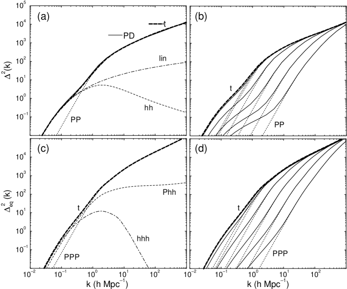
Figure 1.— Dark matter density spectra under the halo prescription. (a) Dark matter power spectrum at the present. (b) Mass cut off effects on the power spectrum. (c) Equilateral bispectrum at the present. (d) Mass cut off effects on the equilateral bispectrum. The power spectrum is compared with the PD fitting function and the linear $P(k)$ in (a). In (b) and (d), from bottom to top, the maximum mass used in the calculation is $10^{11}$, $10^{12}$, $10^{13}$, $10^{14}$, $10^{15}$ and $10^{16}$ M_☉.

2.2. Power Spectrum and Bispectrum

Following Seljak (2000), we can decompose the density power spectrum, as a function of redshift, into contributions from single halos (shot noise or “Poisson” contributions),

$$P^{{\rm P}{\rm P}}(k)=I_{2}^{0}(k,k)\,,$$ (7)

and correlations between two halos,

$$P^{{\rm h}{\rm h}}(k)=\left[I_{1}^{1}(k)\right]^{2}P(k)\,,$$ (8)

such that

$$P^{\rm t}=P^{{\rm P}{\rm P}}+P^{{\rm h}{\rm h}}\,.$$ (9)

As $k\rightarrow 0$, $P^{{\rm h}{\rm h}}\rightarrow P(k)$.

Similarly, we decompose the bispectrum into terms involving one, two and three halos (see Scherrer & Bertschinger 1991; Ma & Fry 2000b):

$$B^{\rm t} = B^{{\rm P}{\rm P}{\rm P}}+B^{{\rm P}{\rm h}{\rm h}}+B^{{\rm h}{\rm h}{\rm h}}\,,$$ (10)

where

$$B^{{\rm P}{\rm P}{\rm P}}(k_{1},k_{2},k_{3})=I_{3}^{0}(k_{1},k_{2},k_{3})\,,$$ (11)

for single halo contributions,

$$B^{{\rm P}{\rm h}{\rm h}}(k_{1},k_{2},k_{3})=I_{2}^{1}(k_{1},k_{2})I_{1}^{0}(k_{3})P(k_{3})+{\rm Perm.}$$ (12)

for double halo contributions, and

$$B^{{\rm h}{\rm h}{\rm h}}(k_{1},k_{2},k_{3}) = \left[2J(k_{1},k_{2},k_{3})I_{1}^{1}(k_{3})+I_{1}^{2}(k_{3})\right]$$

$$\times I_{1}^{1}(k_{1})I_{1}^{1}(k_{2})P(k_{1})P(k_{2})+{\rm Perm.}$$

for triple halo contributions. Here the 2 permutations are $k_{3}\leftrightarrow k_{1}$, $k_{2}$. Second order perturbation theory tells us that (Fry 1984; Bouchet et al 1992; Kamionkowski & Buchalter 1999)

$$J(k_{1},k_{2},k_{3}) = 1-\frac{2}{7}\Omega_{m}^{-2/63}+\left({k_{3}^{2}-k_{1}^{2}-k_{2}^{2}\over 2k_{1}k_{2}}\right)^{2}$$ (14)

$$\times\left[\frac{k_{1}^{2}+k_{2}^{2}}{k_{3}^{2}-k_{1}^{2}-k_{2}^{2}}+\frac{2}{7}\Omega_{m}^{-2/63}\right]\,.$$

As $k\rightarrow 0$, $B^{{\rm h}{\rm h}{\rm h}}\rightarrow B^{\rm PT}$, where $B^{\rm PT}$ is the bispectrum predicted by second-order perturbation theory

$$B^{\rm PT}(k_{1},k_{2},k_{3}) = 2J(k_{1},k_{2},k_{3})P(k_{1})P(k_{2})+{\rm Perm.}\,,$$

with permutations following $k_{3}\leftrightarrow k_{1}$, $k_{2}$.

2.3. Halo Profiles

To apply the halo prescription for the power spectrum and bispectrum, we need to know the profile of the halos. We take the NFW profile (Navarro et al 1996) with a density distribution

$$\rho(r,M)=\frac{\rho_{s}}{(r/r_{s})(1+r/r_{s})^{2}}\,.$$ (16)

The density profile can be integrated and related to the total dark matter mass of the halo within $r_{v}$

$$M=4\pi\rho_{s}r_{s}^{3}\left[\log(1+c)-\frac{c}{1+c}\right]\,,$$ (17)

where the concentration, $c$, is defined as $r_{v}/r_{s}$. Choosing $r_{v}$ as the virial radius of the halo, spherical collapse tells us that $M=4\pi r_{v}^{3}\Delta(z)\rho_{b}/3$, where $\Delta(z)$ is the overdensity of collapse (see e.g. Henry 2000) and $\rho_{b}$ is the background matter density today. We use comoving coordinates throughout. By equating these two expressions, one can eliminate $\rho_{s}$ and describe the halo by its mass $M$ and concentration $c$.

Following Cooray et al (2000b), we take the concentration of dark matter halos to be

$$c(M,z)=a(z)\left[\frac{M}{M_{*}(z)}\right]^{-b(z)}\,,$$ (18)

where $a(z)=10.3(1+z)^{-0.3}$ and $b(z)=0.24(1+z)^{-0.3}$. Here $M_{*}(z)$ is the non-linear mass scale at which the peak-height threshold, $\nu(M,z)=1$. The above concentration is chosen so that dark matter halos provide a reasonable match to the the non-linear density power spectrum as predicted by the Peacock & Dodds (1996); it extends the treatment of Seljak (2000) to the redshifts of interest for lensing. We caution the reader that eqn. (18) is only a good fit for the $\Lambda$CDM model assumed.

2.4. Results

In Fig. 1(a-b), we show the density field power spectrum today ($z=0$), written such that $\Delta^{2}(k)=k^{3}P(k)/2\pi^{2}$ is the power per logarithmic interval in wavenumber. In Fig 1(a), we show individual contributions from the single and double halo terms and a comparison to the non-linear power spectrum as predicted by the Peacock & Dodds (1996) fitting function. In Fig. 1(b), we show the dependence of density field power as a function of maximum mass used in the calculation.

Since the bispectrum generally scales as the square of the power spectrum, it is useful to define

$$\Delta_{\rm eq}^{2}(k)\equiv\frac{k^{3}}{2\pi^{2}}\sqrt{B(k,k,k)}\,,$$ (19)

which represents equilateral triangle configurations, and its ratio to the power spectrum

$$Q_{\rm eq}(k)\equiv{1\over 3}\left[{\Delta_{\rm eq}^{2}(k)\over\Delta^{2}(k)}\right]^{2}\,.$$ (20)

In second order perturbation theory,

$$Q_{\rm eq}^{\rm PT}=1-\frac{3}{7}\Omega_{m}^{-2/63}$$ (21)

and under hyper-extended perturbation theory (HEPT; Scoccimarro & Frieman 1999),

$$Q_{\rm eq}^{\rm HEPT}(k)=\frac{4-2^{n(k)}}{1+2^{n(k)+1}}\,,$$ (22)

which is claimed to be valid in the deeply nonlinear regime. Here, $n(k)$ is the linear power spectral index at $k$.

In Fig. 1(c-d), we show $\Delta_{\rm eq}^{2}(k)$ separated into its various contributions (c) and as a function of maximum mass (d). Since the power spectra and equilateral bispectra share similar features, it is more instructive to examine $Q_{\rm eq}(k)$ (see Fig. 2). Here we also compare it with the second order perturbation theory (PT) and the HEPT prediction. In the halo prescription, $Q_{\rm eq}$ at $k\gtrsim 10k_{\rm nonlin}\sim 10h$Mpc^-1 arises mainly from the single halo term. The HEPT prediction exceeds the halo prediction on larger scales and falls short on smaller scales.

2.5. Discussion

Even though the dark matter halo formalism provides a physically motivated means for calculating the statistics of the dark matter density field, there are several limitations of the approach that should be borne in mind when interpreting the results.

The approach assumes all halos to be spherical with a single profile shape. Any variations in the profile through halo mergers and resulting substructure can affect the power spectrum and higher order correlations. Also, real halos are not perfectly spherical which affects the configuration dependence of the bispectrum.

Furthermore, there are parameter degeneracies in the formalism that prevent a straightforward interpretation of observations in terms of halo properties. For example, one might think that the power spectrum and bispectrum can be used to measure any mean deviation from the assumed NFW profile form. However as pointed out by Seljak (2000), changes in the slope of the inner profile can be compensated by changing the concentration as a function of mass; this degeneracy is also preserved in the bispectrum.

We do not expect these issues to affect our qualitative results. However, if this technique is to be used for precision studies of cosmological parameters, more work will be required in testing it quantitatively against simulations. Studies by Ma & Fry (2000a) and Scoccimarro et al. (2000) show that the bispectrum predictions of the halo formalism are in good agreement with simulations, at least when averaged over configurations. The replacement of individual halos found in numerical simulations with synthetic smooth halos with NFW profiles by Ma & Fry (2000b) show that the smooth profiles can regenerate the measured power spectrum and bispectrum in simulations. This agreement, at least at scales less than 10$k_{\rm nonlin}$, suggests that mergers and substructures may not be important at such scales.

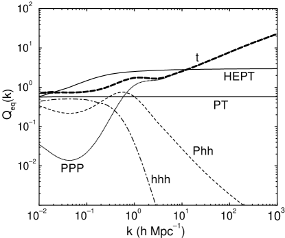
Figure 2.— $Q_{\rm eq}(k)$ at present broken into individual contributions under the halo description and compared with second order perturbation theory (PT) and hyper-extended perturbation theory (HEPT).

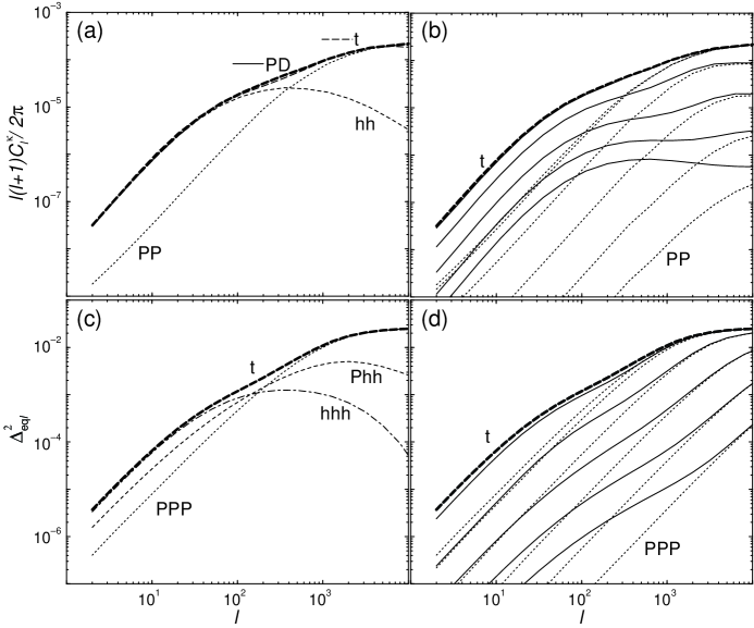
Figure 3.— Weak lensing convergence spectra under the halo description. (a) Angular power spectrum broken into individual contributions. (b) Mass cut off effects on the angular power spectrum. (c) Equilateral bispectrum broken into individual contributions. (d) Mass cut off effects on the equilateral bispectrum. Also shown in (a) is the prediction from the PD nonlinear power spectrum fitting function. The mass cuts are the same as in Fig. 1 and we have assumed that all sources are at $z_{s}=1$.

3. Convergence Power Spectrum and Bispectrum

3.1. Power Spectrum and Variance

The angular power spectrum of the convergence is defined in terms of the multipole moments $\kappa_{lm}$ as

$$\left<\kappa_{lm}^{*}\kappa_{l^{\prime}m^{\prime}}\right>=C_{l}^{\kappa}\delta_{ll^{\prime}}\delta_{mm^{\prime}}\,.$$ (23)

$C_{l}$ is numerically equal to the flat-sky power spectrum in the flat sky limit. It is related to the dark matter power spectrum by (Kaiser 1992; 1998)

$$C^{\kappa}_{l}=\int dr\frac{W(r)^{2}}{d_{A}^{2}}P^{\rm t}\left(\frac{l}{d_{A}};r\right)\,,$$ (24)

where $r$ is the comoving distance and $d_{A}$ is the angular diameter distance. When all background sources are at a distance of $r_{s}$, the weight function becomes

$$W(r)=\frac{3}{2}\Omega_{m}\frac{H_{0}^{2}}{c^{2}a}\frac{d_{A}(r)d_{A}(r_{s}-r)}{d_{A}(r_{s})}\,;$$ (25)

for simplicity, we will assume $r_{s}=r(z_{s}=1)$ throughout. In deriving Eq. (24), we have used the Limber approximation (Limber 1954) by setting $k=l/d_{A}$ and the flat-sky approximation. In Cooray et al (2000b), we used the projected mass of individual halos to construct the weak lensing power spectrum directly. The two approaches are essentially the same since the order in which the projection is taken does not matter.

In Fig. 3, we show the convergence power spectrum of the dark matter halos compared with that predicted by the Peacock & Dodds (1996) power spectrum. The lensing power spectrum due to halos has the same behavior as the dark matter power spectrum. At large angles ($l\lesssim 100$), the correlations between halos dominate. The transition from linear to non-linear is at $l\sim 500$ where halos of mass similar to $M_{\star}(z)$ contribute. The single halo contributions start dominating at $l>1000$.

As shown in Fig. 3(b), and discussed in Cooray et al (2000b), if there is a lack of massive halos in the observed fields convergence measurements will be biased low compared with the cosmic mean. The lack of massive halos affect the single halo contribution more than the halo-halo correlation term, thereby changing the shape of the total power spectrum in addition to decreasing the overall amplitude.

Similar statements apply to variance statistics (second moments) in real space. The variance of a map smoothed with a window is related to the power spectrum by

$$\left<\kappa^{2}(\sigma)\right>={1\over 4\pi}\sum_{l}(2l+1)C_{l}^{\kappa}W_{l}^{2}(\sigma)\,.$$ (26)

where $W_{l}$ are the multipole moments (or Fourier transform in a flat-sky approximation) of the window. For simplicity, we will choose a window which is a two-dimensional top hat in real space with a window function in multipole space of $W_{l}(\sigma)=2J_{1}(x)/x$ with $x=l\sigma$.

In Fig. 4(a-b), we show the second moment as a function of smoothing scale $\sigma$. Here, we have considered angular scales ranging from 5^′ to 90^′, which are likely to be probed by ongoing and upcoming weak lensing experiments. As shown, most of the contribution to the second moment comes from the double halo correlation term and is mildly affected by a mass cut off.

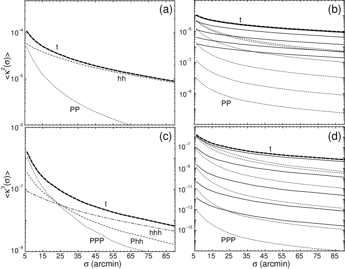
Figure 4.— Moments of the convergence field as a function of top-hat smoothing scale $\sigma$. (a) Second moment broken into individual contributions. (b) Mass cut off effects on the second moments. (a) Third moment broken into individual contributions. (b) Mass cut off effects on the third moments. The mass cuts are the same as in Fig. 1.

3.2. Bispectrum and Skewness

The angular bispectrum of the convergence is defined as

$$\left<\kappa_{l_{1}m_{1}}\kappa_{l_{2}m_{2}}\kappa_{l_{3}m_{3}}\right>=\left(\begin{array}[]{ccc}l_{1}&l_{2}&l_{3}\\ m_{1}&m_{2}&m_{3}\end{array}\right)B_{l_{1}l_{2}l_{3}}^{\kappa}\,.$$ (27)

Extending our derivation of the SZ bispectrum in Cooray et al (2000b), we can write the angular bispectrum of the convergence as

$$B_{l_{1}l_{2}l_{3}}^{\kappa} = \sqrt{(2l_{1}+1)(2l_{2}+1)(2l_{3}+1)\over 4\pi}\left(\begin{array}[]{ccc}l_{1}&l_{2}&l_{3}\\ 0&0&0\end{array}\right)$$ (31)

$$\times\left[\int dr{[W(r)]^{3}\over d_{A}^{4}}B^{\rm t}\left({l_{1}\over d_{A}},{l_{2}\over d_{A}},{l_{3}\over d_{A}};r\right)\right]\,.$$

The more familiar flat-sky bispectrum is simply the expression in brackets (Hu 2000). The basic properties of Wigner-3$j$ symbol introduced above can be found in Cooray et al (2000a).

Similar to the density field bispectrum, we define

$$\Delta^{2}_{{\rm eq}l}=\frac{l^{2}}{2\pi}\sqrt{B^{\kappa}_{lll}}\,,$$ (32)

involving equilateral triangles in $l$-space.

In Fig. 3(c-d), we show $\Delta^{2}_{{\rm eq}l}$. The general behavior of the lensing bispectrum can be understood through the individual contributions to the density field bispectrum: at small multipoles, the triple halo correlation term dominates, while at high multipoles, the single halo term dominates. The double halo term contributes at intermediate $l$’s corresponding to angular scales of a few tens of arcminutes.

In Fig. 5, we show the configuration dependence

$$R_{l_{1}l_{2}}^{l_{3}}={l_{1}l_{2}\over 2\pi}{\sqrt{B^{\kappa}_{l_{1}l_{2}l_{3}}}\over\Delta_{{\rm eq}l}^{2}}\,$$ (33)

as a function of $l_{1}$ and $l_{2}$ when $l_{3}=1000$. The surface, and associated contour plot, shows the contribution to bispectrum from triangular configurations in $l$ space relative to that from the equilateral configuration. Due to the triangular conditions associated with $l$’s, only the upper triangular region of $l_{1}$-$l_{2}$ space contribute to the bispectrum. The symmetry about $l_{1}=l_{2}$ line is due to the intrinsic symmetry associated with the bispectrum. Though the weak lensing bispectrum peaks for equilateral configurations, the configuration dependence is weak.

The skewness is simply one, easily measured, aspect of the bispectrum. It is associated with the third moment of the smoothed map (c.f. eqn. [26])

$$\left<\kappa^{3}(\sigma)\right> = {1\over 4\pi}\sum_{l_{1}l_{2}l_{3}}\sqrt{(2l_{1}+1)(2l_{2}+1)(2l_{3}+1)\over 4\pi}$$ (36)

$$\times\left(\begin{array}[]{ccc}l_{1}&l_{2}&l_{3}\\ 0&0&0\end{array}\right)B_{l_{1}l_{2}l_{3}}^{\kappa}W_{l_{1}}(\sigma)W_{l_{2}}(\sigma)W_{l_{3}}(\sigma)\,.$$

We then construct the skewness as

$$S_{3}(\sigma)=\frac{\left<\kappa^{3}(\sigma)\right>}{\left<\kappa^{2}(\sigma)\right>^{2}}\,.$$ (38)

The effect of the mass cut off is dramatic in the third moment. As shown in Fig 4(c-d), most of the contributions to the third moment come from the single halo term, with those involving halo correlations contributing significantly only at angular scales greater than $\sim$ 25^′. With a mass cut off, the total third moment decreases rapidly and is suppressed by more than three orders of magnitude when the maximum mass drops to $10^{13}$ M_☉. The skewness only saturates when the maximum mass is raised to a few times $10^{15}$ M_☉. Even though a small change in the maximum mass does not greatly change the convergence power spectrum (Fig. 3 of Cooray et al 2000b), the third moment, or the bispectrum, is strongly sensitive to the rarest or most massive dark matter halos.

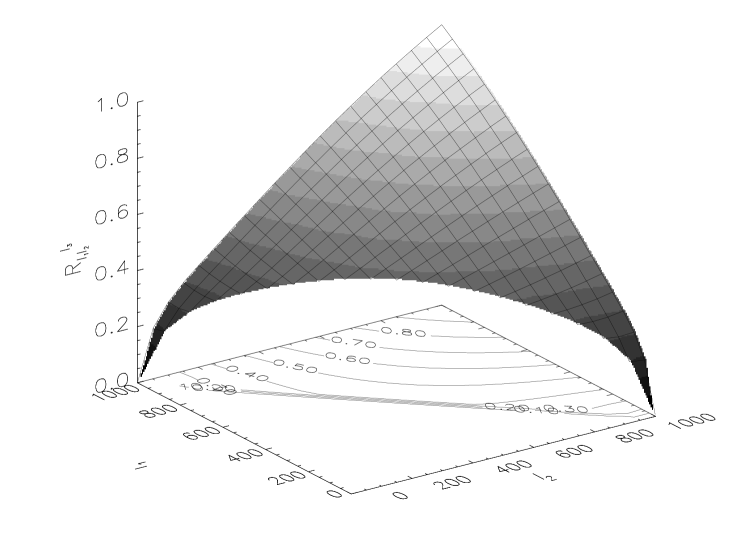
Figure 5.— The bispectrum configuration dependence $R_{l_{1}l_{2}}^{l_{3}}$ as a function of $l_{1}$ and $l_{2}$ with $l_{3}=1000$. Due to triangular conditions associated with $l$’s, only the upper triangular region in $l_{1}$-$l_{2}$ space contribute to the bispectrum.

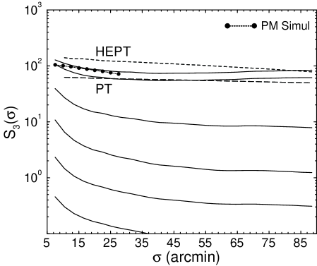
Figure 6.— The skewness, $S_{3}(\sigma)$, as a function of angular scale. Shown here is the skewness values with varying maximum mass as in Fig. 1. For comparison, we also show skewness values as measured in particle-mesh (PM) simulations of White & Hu (1999), as predicted by hyper-extended perturbation theory (HEPT; dashed line) and second-order perturbation theory (PT; long-dashed line).

In Fig. 6 we plot the skewness as a function of maximum mass, ranging from $10^{11}$ to $10^{16}$ M_☉. Our total maximum skewness agrees with what is predicted by numerical particle mesh simulations (White & Hu 1999) and yields a value of $\sim$ 116 at 10^′. However, it is lower than predicted by HEPT arguments and simulations of Jain et al (2000), which suggest a skewness of $\sim$ 140 at angular scales of 10^′. The skewness based on second-order PT is factor of $\sim$ 2 lower than the maximum skewness predicted by halo calculation. As shown, the PT skewness decreases slightly from angular scales of few arcmins to 90^′ and increases thereafter.

The effect of maximum mass on the skewness is interesting. When the maximum mass is decreased to $10^{15}$ M_☉ from the maximum mass value where skewness saturates ($\sim 3\times 10^{15}$ M_☉), the skewness decreases from $\sim$ 116 to 98 at an angular scale of 10^′, though the convergence power spectrum only changes by less than few percent when the same change on the maximum mass used is made. When the maximum mass used in the calculation is $10^{13}$ M_☉, the skewness at 10^′ is $\sim 8$, which is roughly a factor of 15 decrease in the skewness from the total.

The variation in skewness as a function of angular scale is due to the individual contribution to the second and third moments. The increase in the skewness at angular scales less than $\sim$ 30^′ is due to the single halo contributions for the third moment. The triple halo correlation terms dominate angular scales greater than 50^′, leading to a slight increase toward large angles, e.g. from $\sim$ 74 at 40^′ to $\sim$ 85 at 90^′. However, this increase is not present when the maximum mass used in the calculation is less than $\sim 10^{14}$ M_☉. Even though mass cut off affects the single halo contributions more than the halo contribution, at such masses, the change in halo contribution with mass cut off prevents an increase in skewness at large angular scales.

The absence of rare and massive halos in observed fields will certainly bias the skewness measurement from the cosmological mean. One therefore needs to exercise caution in using the skewness to constrain cosmological models Hui 1999). In Cooray et al (2000b), we suggested that lensing observations in a field of $\sim$ 30 deg² may be adequate for an unbiased measurement of the convergence power spectrum. For the skewness, observations within a similar area may be biased by as much as $\sim$ 25%. This is consistent with the sampling errors found in numerical simulations: 1$\sigma$ errors of 24% at $10^{\prime}$ with a 36 deg² field (White & Hu 1999). To obtain the skewness within few percent of the total, one requires a fair sample of halos out to $\sim 3\times 10^{15}$ M_☉, requiring observations of $\sim$ 1000 deg², which is within the reach of upcoming lensing surveys involving wide-field cameras, such as the MEGACAM at Canada-France-Hawaii-Telescope (Boulade et al 1998), and proposed dedicated telescopes (e.g., Dark Matter Telescope; Tyson, private communication).

Still, this does not mean that non-Gaussianity measured in smaller fields will be useless. With this halo approach one can calculate the expected skewness if one knows that the most massive halos are not present in the observed fields. This knowledge may come from external information such as X-ray data and Sunyaev-Zel’dovich measurements or internally from the lensing data.

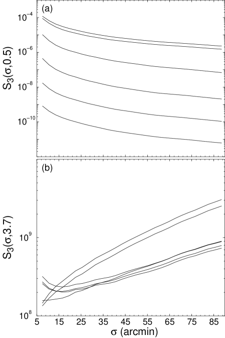
Figure 7.— Generalized skewness statistic $S_{3}(\sigma,m)$. (a) $m=1/2$ following Jain et al (2000). (b) $m=3.7$ chosen to minimize the mass cut off dependence.

3.3. Related Statistics

The halo description in general allows one to test the effect of rare massive halos on any statistic related to the two and three point functions. In particular, it can be used to design more robust statistics.

Generalized three point statistics have been considered previously by Jain et al (2000) following Nusser & Dekel (1993) and Juszkiewicz et al (1995). One such statistic is the $\left<\kappa|\kappa|\right>_{\kappa>0}$, which is expected to reduce the sampling variance from rare and massive halos (see, Jain et al 2000 for details). This statistic is proportional to $\left<\kappa^{3}\right>/\left<\kappa^{2}\right>^{1/2}$. In Fig. 7(a), we show this statistic as a function of maximum mass used in the calculation. We still find strong variations with changes to the maximum mass. Similar variations were also present in other statistics considered by Jain et al (2000).

Consider instead the generalized statistic

$$S_{3}(\sigma,m)=\left<\kappa^{3}\right>/\left<\kappa^{2}\right>^{m}\,$$ (39)

where $m$ is an arbitary index. We varied $m$ such that the effect of mass cuts are minimized on skewness. In Fig. 7(b), we show such an example with $m=3.7$. Here, the values are separated to two groups involving with most massive and rarest halos and another with halos of masses $10^{14}$ M_☉ or less. Though the values from the two groups agree with each other on small angular scales, they depart significantly above $25^{\prime}$ reaching a difference of 2.5 at 80^′. Statistics involving such a high index $m$, weight the single halo contributions highly when the most massive halos are present, whereas they weight the halo correlation terms more strongly for $M<10^{14}$ M_☉. To some extent this may be useful to identify the presence of rare halos in the observations.

However the consequence of using these generalized statistics is that one progressively loses their independence on the details of the cosmological model, e.g. the shape and amplitude of the underlying density power spectrum, as one departs from $m=2$, thereby contaminating the probe of dark matter and dark energy. Further work is necessary find the optimal trade off between robustness and cosmological independence of these and other generalized statistics.

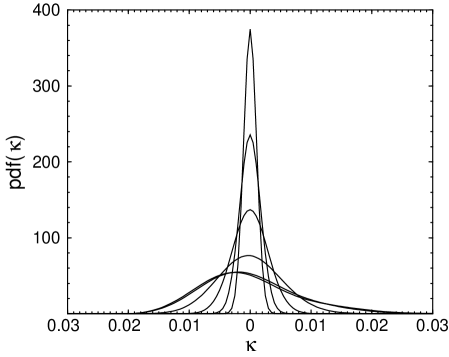
Figure 8.— The probability distribution function of the weak lensing convergence as a function of maximum mass used in the calculation at an angular scale of $12^{\prime}$. From top to bottom, the curves range from $10^{11}$ to $10^{16}$ M_☉.

Another observable statistic is the probability distribution function (pdf) of the convergence maps smoothed on the scale $\sigma$. This possibility has been recently studied by Jain & van Waerbeke (1999), where the reconstruction of pdf using peak statistics were considered. Using the Edgeworth expansion to capture small deviations from Gaussianity, one can write the pdf of convergence to second order as

$$p(\kappa) = \frac{1}{\sqrt{2\pi\left<\kappa^{2}(\sigma)\right>}}\;e^{-\kappa(\sigma)^{2}/2\left<\kappa^{2}(\sigma)\right>}$$

$$\times\left[1+\frac{1}{6}S_{3}(\sigma)\sqrt{\left<\kappa^{2}(\sigma)\right>}H_{3}\left(\frac{\kappa(\sigma)}{\sqrt{\left<\kappa^{2}(\sigma)\right>}}\right)\right]\,,$$

where $H_{3}(x)=x^{3}-3x$ is the third order Hermite polynomial (see, Juszkiewicz et al 1995 for details).

In Fig. 8, we show the pdf of convergence at 12^′ as a function of maximum mass used in the calculation. As shown, the greatest departures from Gaussianity begin to occur when the maximum mass included is greater than $10^{14}$ M_☉. Given that we have only constructed the pdf using terms out to skewness, the presented pdfs should only be considered as approximate. With increasing non-Gaussian behavior, the approximated pdfs are likely to depart from this form especially in the tails. As studied in Jain & van Waerbeke (1999), the measurement of the full pdf can potentially be used a a probe of cosmology. Its low order properties describe deviations from Gaussianity near the peak as opposed to the skewness which is more weighted to the tails.

4. Summary & Conclusions

We have presented an efficient method to calculate the non-Gaussian statistics of lensing convergence at the three point level based on a description of the underlying density field in terms of dark matter halos. The bispectrum contains all of the three point information, including the skewness. The prior attempts at calculating lensing bispectrum and skewness were limited by the accuracy of perturbative approximations and the dynamic range and sample variance of simulations.

Though the present technique provides a clear and an efficient method to calculate the statistics of the convergence field, it has its own shortcomings. Halos are not all spherical, which can to some extent affect the configuration dependence in moments higher than the two point level. Substructures due to mergers of halos can also introduce scatter. Though such effects unlikely to dominate our calculations, further work using numerical simulations will be necessary to determine to what extent present method can be used as a precise tool to study the higher order statistics associated with weak gravitational lensing.

The dark matter halo approach also allows one to study possible selection effects that may be present in weak lensing observations due to the presence or absence of rare massive halos in the small fields that are observed. We have shown that the weak lensing skewness is mostly due to the most massive and rarest dark matter halos in the universe. The effect of such halos is stronger at the three point level than the two point level. The absence of massive halos, with masses greater than $10^{14}$ M_☉, leads to a strong decrease in skewness, suggesting that a straightforward use of measured skewness values as a test of cosmological models may not be appropriate unless prior observations are available on the distribution of masses in observed lensing fields.

One can correct for such biases using the halo approach, however. To implement such a correction in practice, further work will be needed to calibrate the technique precisely against simulations across a wide range of cosmologies. Efficient techniques to correct for mass biases both in the lensing power spectrum and bispectrum will be needed. Alternatively, this technique can be used to search for generalized three point statistics that are more robust to sampling issues. Given the great potential to study the dark matter distribution through weak lensing, this issues merit further study.

References

- (1) Bacon, D., Refregier, A., Ellis R. 2000, MNRAS submitted, astro-ph/0003008
- (2) Bartelmann, M., Schnerider, P. 2000, Physics Reports in press, astro-ph/9912508
- (3) Bernardeau, F., van Waerbeke, L., Mellier, Y. 1997, A&A, 322, 1
- (4) Blandford, R. D., Saust, A. B., Brainerd, T. G., Villumsen, J. V. 1991, MNRAS 251, 60
- (5) Bouchet, F. R., Juszkiewicz, R., Colombi, S. Pellat, R. 1992, ApJ, 394, L5
- (6) Boulade, O., Vigroux, L., Charlot, X. et al. 1998, SPIE, 3355.
- (7) Bunn, E. F., White, M. 1997, ApJ, 480, 6
- (8) Cooray, A. R. 1999, A&A, 348, 673
- (9) Cooray, A., Hu, W., Tegmark, M. 2000a, ApJ in press, astro-ph/0002238
- (10) Cooray, A., Hu, W., Miralda-Escudé, J. 2000b, ApJ in press, astro-ph/0003205
- (11) Eisenstein, D.J. & Hu, W. 1999, ApJ, 511, 5
- (12) Fry, J. N. 1984, ApJ, 279, 499
- (13) Henry, J. P. 2000, ApJ in press, astro-ph/0002365
- (14) Hu W., Tegmark M. 1999, ApJ 514, L65
- (15) Hu, W. 2000, PRD submitted, astro-ph/0001303
- (16) Hui, L. 1999, ApJ, 519, L9
- (17) Jain B., Seljak U. 1997, ApJ 484, 560
- (18) Jain B., van Waerbeke, L. 1999, ApJ in press, astro-ph/9910459
- (19) Jain, B., Seljak, U. & White, M. 2000, ApJ 530, 547
- (20) Juszkiewicz, R., Weinberg, D. H., Amsterdamski, P., Chodorowski, M., Bouchet, F. 1995, ApJ, 442, 39
- (21) Kaiser, N. 1992, ApJ, 388, 286
- (22) Kaiser, N. 1998, ApJ, 498, 26
- (23) Kaiser, N., Wilson, G., Luppino, G.A., 2000, ApJ submitted, astro-ph/0003338
- (24) Kamionkowski, M., Buchalter, A. 1999, ApJ, 514, 7
- (25) Limber, D. 1954, ApJ, 119, 655
- (26) Ma, C.-P., Fry, J. N. 2000a, ApJ, 531, L87
- (27) Ma, C.-P., Fry, J. N. 2000b, ApJ submitted, astro-ph/0003343
- (28) Miralda-Escudé J. 1991, ApJ 380, 1
- (29) Mo, H. J., White, S. D. M. 1996, MNRAS, 282, 347
- (30) Mo, H. J., Jing, Y. P., White, S. D. M. 1997, MNRAS, 284, 189
- (31) Munshi, D. & Jain, B. 1999, MNRAS submitted, astro-ph/9911502
- (32) Navarro, J., Frenk, C., White, S. D. M., 1996, ApJ, 462, 563
- (33) Nusser, A. & Dekel, A. 1993, ApJ, 405, 437
- (34) Peacock, J.A., Dodds, S.J. 1996, MNRAS, 280, L19
- (35) Press, W. H., Schechter, P. 1974, ApJ, 187, 425
- (36) Scherrer, R.J., Bertschinger, E. 1991, ApJ, 381, 349
- (37) Scoccimarro, R. & Frieman, J. 1999, ApJ, 520, 35
- (38) Scoccimarro, R., Sheth, R., Hui, L. & Jain, B. 2000, in preparation.
- (39) Schneider P., van Waerbeke, L., Jain, B., Guido, K. 1998, MNRAS, 296, 873
- (40) Seljak, U. 2000, PRD submitted, astro-ph/0001493
- (41) Van Waerbeke, L., Bernardeau, F., Mellier, Y. 1999, A&A, 342, 15
- (42) Van Waerbeke, L., Mellier, Y., Erben, T. et al. 2000, A&A submitted, astro-ph/0002500
- (43) Viana, P. T. P., Liddle, A. R. 1999, MNRAS, 303, 535
- (44) White, M., Hu, W. 1999, ApJ, in press, astro-ph/9909165
- (45) Wittman, D. M., Tyson, J. A., Kirkman, D., Dell’Antonio, I., Bernstein, G. 2000, Nature submitted, astro-ph/0003014