Properties of cosmologies with dynamical pseudo Nambu–Goldstone bosons

Abstract

We study observational constraints on cosmological models with a quintessence field in the form of a dynamical pseudo Nambu–Goldstone boson. After reviewing the properties of the solutions, from a dynamical systems phase space analysis, we consider the constraints on parameter values imposed by luminosity distances from the 60 type Ia supernovae published by Perlmutter et al., and also from gravitational lensing statistics of distant quasars. In the case of the type Ia supernovae we explicitly allow for the possibility of evolution of the peak luminosities of the supernovae sources, using simple empirical models which have been recently discussed in the literature. We find weak evidence to suggest that the models with supernovae evolution fit the data better in the context of the quintessence models in question. If source evolution is a reality then the greatest challenge facing these models is the tension between current value of the expansion age, $H_{0}t_{0}$, and the fraction of the critical energy density, $\Omega_{\phi 0}$, corresponding to the scalar field. Nonetheless there are ranges of the free parameters which fit all available cosmological data.

I Introduction

Scalar fields have played a central role in models of the very early universe for the past 20 years. In the past few years attention has turned to models in which a scalar field plays a dynamical role at late times, rather than simply being frozen in as a static relic vacuum energy. Such models, which have been dubbed “quintessence” models [3], could in principle provide a dynamical solution to the cosmological constant problem – namely the question of why the magnitude of the vacuum energy at the present epoch is so much smaller than one might naïvely expect from particle physics models such as various supergravity theories. A dynamical ‘solution’ of the cosmological constant problem would amount to a demonstration that a particular dynamical evolution of the scalar quintessence field is a natural consequence of the cosmological field equations without fine-tuning of parameters, given some reasonable physical assumptions about the initial conditions.

The most notable recent observational evidence which has driven the theoretical interest is the measurement of the apparent magnitude-redshift relationship using type Ia supernovae (SNe Ia) [4]. These results have been interpreted, in the context of a cosmological model containing pressureless dust and a cosmological constant, $\Lambda$, as evidence that the universe is undergoing accelerated expansion at the present epoch (see [5, 6] and references therein). The validity of this conclusion is currently open to some doubt, however. In particular, a recent analysis by Riess et al. [7] indicates that the sample of type Ia supernovae shows a possible evolution in rise times from moderate ($z\mathop{\sim}\limits 0.3$) to large ($z\mathop{\sim}\limits 1$) redshifts. Although the statistical significance of this result has been diminished – from the $5.8\sigma$ level [7] to the $1.5\sigma$ level [8] – upon a more rigorous treatment of the uncertainties in the data [8], it remains true that while a systematic evolution in the rise times of the supernovae is not conclusively ruled in, neither is it conclusively ruled out.

Given that an evolution in the shape of the light curves of the supernovae measured in their rest frame remains a real possibility, it would not be surprising if the peak luminosity – which is the effective standard candle used – were also to evolve. Riess et al. [7] conclude that the type Ia supernovae data could conceivably be explained entirely within the context of an open Friedmann-Robertson-Walker universe together with a reasonable astrophysical evolution model, e.g., a consequence of a time variation of the abundances of relevant heavy elements in the environment of the white dwarf supernovae progenitors. Detailed astrophysical modelling – see, e.g., [9] – should hopefully eventually resolve the issue, although at this stage the difference between our theoretical understanding and the observations remains quite substantial [10].

In many recent papers it has been commonly assumed that the dynamical scalar field, $\phi$, should obey an effective equation of state $P_{\phi}\simeq w\rho_{\phi}$ with $-1<w<0$, at the present epoch, in order to obtain a cosmological acceleration, i.e., a negative deceleration parameter $q_{0}$. Indeed, the condition that $-1<w<0$ is often taken as a defining characteristic of “quintessence” [3]. The broad picture in this cosmological scenario is that the universe is currently in the early stage of an epoch of inflationary expansion. The motivation for this is that one could then hope to have a model cosmology in which observations such as the type Ia supernovae apparent magnitude–redshift relation could be explained by a cosmological acceleration in a similar fashion to models with a cosmological constant, but with the possibility of explaining why the magnitude of the vacuum energy density and the energy density in ordinary pressureless matter, $\rho_{m}$, are comparable at the present epoch – the so-called “cosmic coincidence problem” [11].

One attractive feature of homogeneous isotropic cosmological models with dynamical scalar fields is that many of them possess “cosmological scaling solutions” [12], namely solutions which at late times have energy density components which depend on the cosmic scale factor according to $\rho\propto a^{-m_{1}}$ and $\rho_{\phi}\propto a^{-m_{2}}$ simultaneously, and which act as attractors in the phase space. If $m_{2}<m_{1}$, which is the case, for example, for simple power-law potentials with inverse powers [13, 14] $V(\phi)\propto\phi^{-\alpha}$, or for certain power-law potentials with positive powers [12] then the scalar field dominates at late times, producing a quintessence-dominated cosmology with accelerated expansion at late times. If $m_{1}=m_{2}$, which is the case for exponential potentials [15, 16, 17, 18, 19, 20, 21, 22], then the scaling solutions are “self-tuning” [18] – i.e., the dynamics of the scalar field follows that of the other dominant energy component, with a dependence $\rho_{\phi}\propto a^{-4}$ in the radiation–dominated era and a dependence $\rho_{\phi}\propto a^{-3}$ in the matter–dominated era.

Even if the ultimate late-time behaviour properties of the solutions is not precisely “self-tuning” in the above sense, models such as those with inverse power law potentials can still effectively act as “tracking solutions”, since for a wide range of initial conditions, the solutions rapidly converge to a common, cosmic evolutionary track [14]. Thus there are a number of ways in which one might hope to solve the “cosmic coincidence problem”, though in practice a degree of tuning of the parameters has been necessary in all models studied to date.

In this paper, we consider a form of quintessence, an ultra-light pseudo Nambu-Goldstone-boson (PNGB) [23] which is still relaxing to its vacuum state. From the viewpoint of quantum field theory PNGB models are the simplest way to have naturally ultra-low mass, spin-$0$ particles and hence perhaps the most natural candidate for a presently-existing minimally-coupled scalar field. The effective potential of a PNGB field $\phi$ can be taken to be of the form [24]

$$V(\phi)=M^{4}[\cos(\phi/f)+1]\ ,$$ (1)

where the constant term is to ensure that the vacuum energy vanishes at the minimum of the potential. This potential is characterized by two mass scales, a purely spontaneous symmetry breaking scale $f$ and an explicit symmetry breaking scale $M$.

The effective PNGB mass is $m_{\phi}\mathop{\sim}\limits M^{2}/f$. To obtain solutions with $\Omega_{\phi}\mathop{\sim}\limits 1$, the energy scales are essentially fixed [23] to values $M\mathop{\sim}\limits 10^{-3}\;\hbox{eV}\;$, interestingly close to the neutrino mass scale for the MSW solution to the solar neutrino problem, and $f\mathop{\sim}\limits m_{PL}\simeq 10^{19}\;\hbox{GeV}\;$, the Planck scale. Since these two energy scales have values which are reasonable from the viewpoint of particle physics, one might hope to explain the coincidence that the vacuum energy is dynamically important at the present epoch.

The cosmology of PNGB models has already been extensively studied in the literature [19, 20, 22, 24, 25, 26]. In particular, a number of constraints have been placed on the parameters $M$ and $f$ by various sets of observational data [19, 20, 25, 26]. Most recently, Frieman and Waga [26] have set bounds based on the SNe Ia data of Riess et al.[6] (hereafter R98) on the one hand, and gravitational lensing surveys on the other. Comparing these bounds is of interest, since the SnIa data have been interpreted as favouring a cosmological constant, whereas gravitational lensing data has been used to place upper bounds on $\Lambda$ [27, 28, 29]. They therefore provide complementary tests of the parameter spaces of models with a non-trivial vacuum energy.

In this paper it is our intention to critically study these bounds. Firstly, we will consider how the bounds are affected by the initial value of the scalar field at the beginning of the matter–dominated epoch. Secondly, we wish to investigate how such bounds might be affected in the case of the PNGB model if the observed apparent faintness of type Ia supernovae is at least partly due to an intrinsic evolution of the sources over cosmological time scales, which in view of the results of [7] would appear to be a very real possibility. The reason for focusing on the PNGB models in such an investigation is suggested by the fact that whereas many quintessence models have been singled out in the literature, perhaps somewhat artificially, simply because they have the property of yielding an accelerated expansion, many different possibilities arise in the PNGB case. Indeed, at very late times, the apparent magnitude–redshift relation for PNGB models ultimately coincides with that of the Einstein–de Sitter model, even though the density of ordinary matter can be low in the PNGB cosmologies. The requirement that the faintness of type Ia supernovae is entirely due to their cosmological distances places rather strong restrictions on the values of the parameters $M$ and $f$ [26], because it requires us to exist at an epoch of the PNGB cosmologies which is still quite far removed from our ultimate destiny. If these restrictions are relaxed because of evolutionary effects, then it is quite plausible that other regions of the parameter space of the PNGB models become viable alternatives. Since PNGB cosmologies could therefore still solve the “missing energy problem”, even if the evidence for a cosmological acceleration proves to be ephemeral, we believe it is important to investigate this possibility quantitatively.

We will begin the paper with a qualitative analysis of the solutions, to provide some general insights which will help to guide our quantitative discussion. Although these properties are no doubt already known, to the best of our knowledge an analysis of the phase space of the solutions has never been presented in the literature. Having completed this analysis in Sec. II we will go on to discuss a number of issues relating to numerical integration in Sec. III, and relate the properties of the solutions found numerically to the exact analysis of Sec. II. In Sec. IV we present the main analysis of the constraints imposed on the $(M,f)$ parameter space, allowing for the possibility of evolution of peak luminosities in the type Ia supernova sources. Bounds from gravitational lensing statistics are updated in Sec. V, and the implications of our results are discussed at greater length in Sec. VI.

II Phase-Space Analysis

We will begin by performing an analysis of the differential equations governing the cosmological evolution in a manner similar to previous studies in inflationary and quintessential models [12, 16, 17, 21, 22].

The classical action for gravity coupled to a scalar field $\phi$ has the form

$$S=\int d^{4}x\sqrt{-g}\left[\left({R\over 2\kappa^{2}}-{1\over 2}g^{\mu\nu}\partial_{\mu}\phi\,\partial_{\nu}\phi-V(\phi)\right)+{\cal L}\right],$$ (2)

where $\kappa$ is the Planck constant, $R$ is the Ricci scalar, $g\equiv\det{g_{\mu\nu}}$, and $L$ is the Lagrangian density of non-relativistic matter and radiation. For simplicity, we assume $\phi$ is minimally coupled to the curvature, and we work in units in which $\hbar=c=1$.

Consider a spatially-flat Friedmann-Robertson-Walker (FRW) universe containing a fluid with barotropic equation of state $P_{\gamma}=(\gamma-1)\rho_{\gamma}$, where $\gamma$ is a constant, $0\leq\gamma\leq 2$, such as radiation ($\gamma=4/3$) or dust ($\gamma=1$). There is a self-interacting scalar field with the PNGB potential energy density (1) evolving in this universe. The total energy density of this homogeneous scalar field is $\rho_{\phi}=\dot{\phi}^{2}/2+V(\phi)$. The governing equations are given by

$$\dot{H} = -{\kappa^{2}\over 2}\left(\rho_{\gamma}+P_{\gamma}+\dot{\phi}^{2}\right)\ ,$$ (3)

$$\dot{\rho_{\gamma}} = -3H(\rho_{\gamma}+P_{\gamma})\ ,$$ (4)

$$\ddot{\phi} = -3H\dot{\phi}-{dV\over d\phi}\ ,$$ (5)

subject to the Friedmann constraint

$$H^{2}={\kappa^{2}\over 3}\left(\rho_{\gamma}+{1\over 2}\dot{\phi}^{2}+V\right)\ ,$$ (6)

where $\kappa^{2}\equiv 8\pi G$, $H=\dot{a}/a$ is the Hubble parameter, and an overdot denotes ordinary differentiation with respect to time $t$.

We may rewrite the Friedmann constraint as

$$\Omega_{\gamma}+\Omega_{\phi}=1$$ (7)

where

$$\Omega_{\gamma} = {\kappa^{2}\rho_{\gamma}\over 3H^{2}}\ ,$$ (8)

$$\Omega_{\phi} = {\kappa^{2}\over 3H^{2}}\left({1\over 2}\dot{\phi}^{2}+V\right)$$ (9)

are the ratios of the energy densities of the barotropic matter and the quintessence field as fraction of the critical density respectively.

In contrast to the case of the cosmologies with an exponential potential [16, 17, 21] where the dynamics can be reduced to a 2-dimensional autonomous phase plane, for the system (3) - (6) the simplest phase space appears to be 3-dimensional in the full four-dimensional phase space.

There are two alternative choices of variables which are useful to describe the dynamics, which we will discuss in turn.

A Field Variables

The first choice is to simply use the Hubble parameter, H, the scalar field and its first derivative as the elementary variables. These are of course simply the variable $u$, $v$, $w$ of Frieman and Waga [20] up to an overall scaling. By defining

$$I\equiv{\phi\over f}={\kappa\phi\over{\cal F}}\ ;\qquad J\equiv\kappa\dot{\phi}\ ;\qquad$$ (10)

we therefore obtain the system

$$\dot{H} = -{3\gamma\over 2}H^{2}+{\gamma m^{2}\over 2}(\cos{I}+1)-{(2-\gamma)\over 4}J^{2}\ ,$$ (11)

$$\dot{I} = {J\over{\cal F}}\ ,$$ (12)

$$\dot{J} = -3HJ+{m^{2}\over{\cal F}}\sin{I}\ ,$$ (13)

where for notational simplicity we define $m^{2}=\kappa^{2}M^{4}$, and ${\cal F}=\kappa f$. so that ${\cal F}$ is dimensionless, while $m$ has dimensions inverse time. The constraint equation becomes

$$\kappa^{2}\rho_{\gamma}=3H^{2}-m^{2}(\cos{I}+1)-{1\over 2}J^{2}\ .$$ (14)

From Eq. (4), it follows that $\dot{\rho_{\gamma}}=0$ if $\rho_{\gamma}=0$. Therefore trajectories do not cross the 2-dimensional $\rho_{\gamma}=0$ surface, which is a hyperboloid in the variables $H$, $\cos(I/2)$, and $J$. Physical trajectories with $\rho_{\gamma}>0$ are forced to lie within the volume of the $H$, $I$, $J$ phase space bounded by the $\rho_{\gamma}=0$ surface.

The only critical points of the system (11)-(13) at finite values of $H$, $I$, $J$ occur at

1. ${\rm C}_{1\pm}$ at $H=\pm{H_{1}}$, $I=0$ mod $2\pi$, $J=0$; and

2. ${\rm C}_{2}$ at $H=0$, $I=\pi$ mod $2\pi$, $J=0$,

where

$${H_{1}}\equiv\sqrt{\frac{2}{3}}\,m$$ (15)

Both of these points in fact lie on the $\rho_{\gamma}=0$ surface. Furthermore, this surface intersects the $H=0$ plane only at the isolated points ${\rm C}_{2}$. The $H>0$ and $H<0$ subspaces are thus physically distinct, and the $H<0$ subspace simply correspond to the time-reversal of the $H>0$ subspace. Therefore we can take $H>0$ without loss of generality.

The pattern of trajectories close to the $\rho_{\gamma}=0$ surface can be ascertained by continuity to the $\rho_{\gamma}=0$ solutions, even though the latter are not physical. The $\rho_{\gamma}=0$ subspace is obtained, for example, by regarding (14) as a quadratic equation for $H$, and using the solution to eliminate $H$, thereby obtaining a 2-dimensional system for $I$ and $J$ given by (12) and (13).

We plot the resulting $H>0$ pattern of trajectories in Fig. 1 for values of $I\in[0,2\pi)$. Since the potential, $V(\phi)$, is periodic the same pattern of trajectories repeats itself as we extend $I$ to $\pm\infty$, with trajectories crossing from one “cell” to another at the cell boundaries.

FIG. 1.: The projection of the trajectories within the $\rho_{\gamma}=0$ subspace on the $I$ – $J$ plane for values of $I\in[0,2\pi)$. Within this subspace, ${\rm C}_{1+}$ is a saddle point and ${\rm C}_{2}$ is a stable spiral.

The trajectories which occupy the lower half of Fig. 1 are obtained from those in the upper half by the symmetry $I\rightarrow 2\pi-I$, $J\rightarrow-J$ of the differential equations (11) - (14). Physically this simply corresponds to the scalar field rolling from the maximum to the right of the minimum as opposed to the one to the left.

An analysis of small perturbations about the critical points ${\rm C}_{1}$ and ${\rm C}_{2}$ yield eigenvalues

1. $\lambda=-\sqrt{6}m\gamma,-{m\over 2}\left(\sqrt{6}\pm\sqrt{6+4/{\cal F}^{2}}\right)$ at ${\rm C}_{1+}$,

2. $\lambda=0,\pm{im\over{\cal F}}$ at ${\rm C}_{2}$.

Thus ${\rm C}_{1+}$ attracts a two-dimensional bunch of trajectories but is a saddle point with respect to trajectories lying in the $\rho_{\gamma}=0$ surface, as is evident from Fig. 1. The 2-dimensional bunch of trajectories which approach ${\rm C}_{1+}$ are found to correspond to inflationary solution with $a\propto\exp(\sqrt{2/3}mt)$ as $t\rightarrow\infty$ and $\phi\rightarrow$ const $=2n\pi{\cal F}$, $n\in$ Z. The possible role of scalar fields with PNGB potentials in driving an inflationary expansion of the early universe has been discussed in [30].

The point ${\rm C}_{2}$ is a degenerate case, in particular with regard to perturbations orthogonal to the $\rho_{\gamma}=0$ surface, (i.e. into the surface $\rho_{\gamma}>0$ region), for which the eigenvalue is zero. It is a centre with respect to the trajectories lying in the $\rho_{\gamma}=0$ surface, and when perturbations of higher order are considered it becomes a stable spiral point in the $\rho_{\gamma}=0$ surface as can be seen in Fig. 1. Since there is a degeneracy, however, an alternative choice of phase space variables is desirable. We will defer a discussion of the late time behaviour of the solution near ${\rm C}_{2}$ to Sec. II B.

The points ${\rm C}_{1\pm}$ correspond to models with a scalar field sitting at the maximum of the potential, whereas ${\rm C}_{2}$ corresponds to the scalar field sitting at the bottom of the potential well. The separatrices in Fig. 1 which join ${\rm C}_{1\pm}$ to ${\rm C}_{2}$ correspond to the field rolling from the maximum to the minimum. It would appear from Fig. 1 trajectories which spiral into ${\rm C}_{2}$ become arbitrarily close to the separatrix at late times.

The separatrices which join the points ${\rm C}_{1\pm}$ to points at infinity correspond to solutions for which the scalar field reaches the top of the potential hill as $t\rightarrow\pm\infty$, (e.g., the rightmost trajectory in Fig. 1). Finally, there are also straight line separatrices parallel to the $H$-axis at each of the points ${\rm C}_{1\pm}$, extending from $H=\pm H_{1}$ to infinity, which represent solutions with a static scalar field sitting on top of the potential hill.

To examine the critical points at infinity it is convenient to transform to spherical polar coordinates $r$, $\theta$, and $\phi$ by defining

$$H = r\cos\theta\ ,$$ (16)

$$I = r\sin\theta\sin\phi\ ,$$ (17)

$$J = r\sin\theta\cos\phi,$$ (18)

and to bring the sphere at infinity to a finite distance from the origin by the transformation $r=\rho/(1-\rho)$, $0\leq\rho\leq 1$ [31].

Although the trajectories on the sphere at infinity do not represent physical cosmologies, it is useful to plot them since the form of the trajectories which lie just within the sphere will be similar. On the sphere $\rho=1$ we find

$${d\theta\over d\xi} = \sin\theta\cos^{2}\theta\left[3\sin^{2}\phi+{2-\gamma\over 4}(\tan^{2}\theta\cos^{2}\phi-6)\right],$$ (19)

$${d\phi\over d\xi} = {3\over 2}\cos\theta\sin{2\phi},$$ (21)

where $\xi$ is a new time coordinate defined by $d\xi=rdt$. The resulting integral curves are plotted in Fig. 2. By (14) the projection of the physical region $\rho_{\gamma}>0$ onto the sphere at infinity leads to the condition

$$\cot^{2}\theta>{1\over 6}\cos^{2}\phi.$$ (22)

Values of $\theta$ and $\phi$ which violate this inequality lie in the shaded region.

FIG. 2.: The projection of trajectories within the sphere at infinity on the $\phi$ – $\theta$ plane. The unphysical region is shaded.

The critical points on the sphere at infinity are

1. ${\rm A}_{1\pm}^{\infty}$, ${\rm A}_{2\pm}^{\infty}$: four points at

   $(\theta,\phi)\in\{(\pm\tan^{-1}\sqrt{6},0),(\pm\tan^{-1}\sqrt{6},\pi)\}$ or

   $H=\pm\infty$, $I/H=0$, and $J/H=\pm\sqrt{6}$.

2. ${\rm B}_{\pm}^{\infty}$: two points at

   $H=\pm\infty$, $I/H=0$, and $J/H=0$.

   Since the projection onto spherical polar coordinates (16) - (18) is degenerate at the north and south poles $\theta=0,\pi$, these points are excluded from the chart $(\theta,\phi)$ but can be included using an alternative hemispherical projection (see Fig. 3).

3. ${\rm C}_{1,2}^{\infty}$: two points at

   $(\theta,\phi)\in\{(\pi/2,\pi/2),(\pi/2,3\pi/2)\}$ or

   $I=\pm\infty$, $H/I=0$, and $J/I=0$.

FIG. 3.: The projection of trajectories within the $I>0$ and $I<0$ hemispheres at infinity on the $H$ – $J$ plane. The unphysical region is shaded.

TABLE I.: The critical points on the sphere at infinity and their eigenvalues.

Critical points	Eigenvalues (with degeneracies)
${\rm A}_{1\pm}^{\infty}$, ${\rm A}_{2\pm}^{\infty}$	$\pm 3$ (2), $\pm 3(2-\gamma)$
${\rm B}_{\pm}^{\infty}$	$\pm{3\gamma\over 2}$ (2), $\mp{3\over 2}(2-\gamma)$
${\rm C}_{1,2}^{\infty}$	0 (3)

An analysis of small perturbations shows that the points ${\rm A}_{1+,2+}^{\infty}$ are repellors in all directions of the phase space (cf., Table I), while ${\rm A}_{1-,2-}^{\infty}$ are attractors. This therefore represents the most ‘typical’ early behaviour of solutions. For $H>0$, ${\rm A}_{1+,2+}^{\infty}$ correspond to the limit $t\rightarrow 0$. We find that $H\mathop{\sim}\limits{1\over 3t}$ or $a\propto t^{1/3}$, while $\kappa\phi\mathop{\sim}\limits\pm\sqrt{2/3}\ln t$, for these solutions. The points ${\rm A}_{1-,2-}^{\infty}$ with $H<0$ represent the time-reversed solutions.

The point ${\rm B}_{+}^{\infty}$ (${\rm B}_{-}^{\infty}$) repels (attracts) a 2-dimensional bunch of trajectories travelling to (from) finite values of $H$, $I$, $J$, but is a saddle point with respect to directions on the sphere at infinity. The points are found to correspond to $t\rightarrow 0$ with $H\mathop{\sim}\limits{2\over 3\gamma t}$ or $a\propto t^{2/3\gamma}$ while $\kappa\phi\propto t^{n}$, $n>0$.

The points ${\rm C}_{1,2}^{\infty}$ are the projection of the points ${\rm C}_{1\pm}$ and ${\rm C}_{2}$ into the sphere at infinity. The degenerate eigenvalues simply reflect the degeneracy of the projection.

${\rm B}_{+}^{\infty}$ acts as a repellor for trajectories with $\dot{\phi}\simeq 0$, $\phi\simeq$ const as $t\rightarrow 0$. As shown in Fig. 3, trajectories are driven towards ${\rm B}_{+}^{\infty}$ before they reach ${\rm C}_{1}^{\infty}$. This is consistent with the property that when $H$ is large ($3H\geq m_{\phi}$), the field evolution is over-damped by the expansion, and the field is effectively frozen to its initial value ($\dot{\phi}\rightarrow 0$).

B Energy Density Variables

In view of the eigenvalue degeneracy encountered above, we can alternatively choose to represent the system by the variables $H$, $x$, and $y$, where

$$x \equiv {\kappa\dot{\phi}\over\sqrt{6}H}={J\over\sqrt{6}H}\ ,$$ (23)

$$y \equiv {\kappa\sqrt{V}\over\sqrt{3}H}={\sqrt{2}m\cos(I/2)\over\sqrt{3}H}\ .$$ (24)

These are the same variables used by Copeland, Liddle and Wands [21] for the model with an exponential potential. As above, we will consider $H>0$ only. The field equations then take the form

$$\dot{H} = -{3\over 2}H^{2}\mu\ ,$$ (25)

$$\dot{x} = \pm{my\over{\cal F}}\sqrt{1-{3y^{2}H^{2}\over 2m^{2}}}+{3\over 2}Hx(\mu-2)\ ,$$ (26)

$$\dot{y} = \mp{mx\over{\cal F}}\sqrt{1-{3y^{2}H^{2}\over 2m^{2}}}+{3\over 2}Hy\mu\ ,$$ (27)

where

$$\mu(x,y)\equiv\gamma(1-y^{2})+(2-\gamma)x^{2}\ .$$ (28)

We note that in these variables

$$x^{2}+y^{2}=\Omega_{\phi}$$ (29)

which is why we have adopted the terminology “energy density variables”. The physical region of the phase space will be constrained to lie within the cylinder $x^{2}+y^{2}\leq 1$ since $\Omega_{\phi}\leq 1$. In the case of the exponential potential analysed in Ref. [21], one of the differential equations decoupled, and the dynamics was effectively described by a phase plane with trajectories bounded by the circle $x^{2}+y^{2}=1$. In the present case, however, no such simplification arises.

The physical region of phase space is further restricted by the requirement that $y^{2}\leq\frac{2}{3}m^{2}/H^{2}\equiv{H_{1}}^{2}/H^{2}$, which is equivalent to $\cos^{2}\left(I/2\right)\leq 1$ in terms of the field variables. For values of $H>{H_{1}}$ each $H=\hbox{const}$ slice of the cylinder $x^{2}+y^{2}\leq 1$ is cut off in the $y$-direction above and below the $y=\pm{H_{1}}/H$ lines. Thus the “fundamental cell” of the phase space can be considered to be a cylinder for $0\leq H\leq{H_{1}}$, capped by a horn for $H>{H_{1}}$, which tapers off to a line segment $-1\leq x\leq 1$ on the $x$-axis as $H\rightarrow\infty$ (see Fig. 4). In fact, the phase space consists of an infinite number of copies of the fundamental cell of Fig. 4 as a result of the periodic structure of the potential. These cells, ${\cal C}_{n}$, can be labelled by an integer, $n$, with the variable $I$ lying in the range $2n\pi\leq I<2(n+1)\pi$ for each $n$. For cells with even $n$ the dynamics is described by (25)–(28) with the upper sign in (26) and (27), while for odd $n$ one must take the lower sign.

FIG. 4.: The “fundamental cell” of the phase space in terms of the energy density variables. On the $y^{2}=H_{1}^{2}/H^{2}$ planes (The shaded planes), only one trajectory is possible as shown. It corresponds to the scalar field lying on top of the potential hill all along. On the $H=0$ plane, the trajectories are concentric circles with centre at the origin.

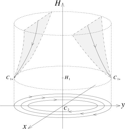
Within the horn portion of each phase space cell the motion of most trajectories is roughly circular in $H=\hbox{const}$ slices, in a clockwise sense in even cells, ${\cal C}_{2n}$, and anti-clockwise in odd cells ${\cal C}_{2n+1}$. However, trajectories can cross from one cell to another along the $y=\pm{H_{1}}/H$ boundaries of their horns, which correspond to the surfaces $I=2n\pi$ in terms of the field variables. For even cells, ${\cal C}_{2n}$, trajectories join the cell ${\cal C}_{2n}$ along the $y={H_{1}}/H$ surface and the cell ${\cal C}_{2n+1}$ along the $y=-{H_{1}}/H$ surface. Below the $H={H_{1}}$ plane solutions cannot cross from one cell to another, but remain confined within the cylinder $x^{2}+y^{2}\leq 1$.

When $H=0$ we see from (25) - (28) that $\dot{x}=my/{\cal F}$ and $\dot{y}=-mx/{\cal F}$, so that trajectories which lie in the $H=0$ surface are purely concentric circles. Since $\dot{a}=0$ in the $H=0$ plane, these do not represent physically interesting cosmologies, but by continuity the behaviour of the trajectories just above the plane will be of a spiral nature.

The origin $H=x=y=0$ is in fact the critical point corresponding to ${\rm C}_{2}$. The nature of the critical point is altered by the change of variables, however. In particular, whereas the eigenvalues for linear perturbations are unchanged, when higher order corrections are considered the point is no longer always an asymptotically stable spiral as was the case in Fig. 1.

Asymptotically as $t\rightarrow\infty$ we have

$$x=A(t)\sin{mt\over{\cal F}}\ ,$$ (30)

$$y=A(t)\cos{mt\over{\cal F}}\ ,$$ (31)

where the amplitude is governed by the equation

$${d\over dt}(A^{2})=3HA^{2}\left(\gamma-2\sin^{2}{mt\over{\cal F}}\right)(1-A^{2})\ .$$ (32)

The nature of ${\rm C}_{2}$ is now found to depend on $\gamma$:

1. If $\gamma<1$ we find that over a cycle the average value of the r.h.s. of (32) is negative and $A^{2}$ decreases so that ${\rm C}_{2}$ is an asymptotically stable spiral. Furthermore to leading order $H\mathop{\sim}\limits{2\over 3\gamma t}$ as $t\rightarrow\infty$ or $a\propto t^{2/3\gamma}$ and $A(t)$ is given by

   $$A(t)=Bt^{(\gamma-1)/\gamma}\exp\left[-{1\over\gamma}\int^{\infty}_{t}{{dt^{\prime}\over t^{\prime}}\cos\left({mt^{\prime}\over{\cal F}}\right)}\right]$$ (33)

   with $B$ constant. The late-time attractor has $\Omega_{\phi}=0$ and $\Omega_{\gamma}=1$

2. If $\gamma>1$ then over a cycle the average value of the r.h.s. of (32) is positive and $A^{2}$ increases until it reaches a limit cycle $A^{2}=1$, i.e. $x^{2}+y^{2}=1$ or $\Omega_{\phi}=1$, $\Omega_{\gamma}=0$. In this case

   $$A(t)=1-\bar{B}t^{2(1-\gamma)}\exp\left[-2\int^{\infty}_{t}{{dt^{\prime}\over t^{\prime}}\cos\left({mt^{\prime}\over{\cal F}}\right)}\right]\ .$$ (34)

3. If $\gamma=1$, which corresponds physically to an ordinary matter-dominated universe, then an intermediate situation obtains. Essentially any of the concentric circles in the $H=0$ plane of Fig. 4 can be approached asymptotically giving a universe for which $\Omega_{\phi}\rightarrow\alpha_{1}$ and $\Omega_{\phi}\rightarrow 1-\alpha_{1}$ where $\alpha_{1}$ is a constant in the range $0<\alpha_{1}<1$, which depends on the initial conditions and the parameters $m$ and ${\cal F}$.

We observe that for all values of $\gamma$,

$$\rho_{\phi}\propto{1\over a^{3}}$$ (35)

at late times. Since $\rho_{\gamma}\propto a^{-3\gamma}$, the three different late time behaviours can thus be understood as a consequence of the scalar field either decreasing more rapidly than the barotropic fluid ($\gamma<1$), less rapidly ($\gamma>1$), or at the same rate ($\gamma=1$). The scalar field thus eventually dominates if $\gamma>1$, while the barotropic fluid dominates if $\gamma<1$. In the interesting critical case of dust filled models ($\gamma=1$) both the scalar field and ordinary matter are of cosmologically significant density at late times.

One simplification that is often made in studying quintessence models is to assume that at late times the quintessence field obeys an equation of state

$$P_{\phi}=\left(\gamma_{\phi}-1\right)\rho_{\phi}$$ (36)

with $\gamma_{\phi}$ effectively constant. While such an assumption is justified in the case of models with a slowly varying scalar field, it does not apply in the present case. In particular, since the effective barotropic index of the scalar field is [17]

$$\gamma_{\phi}={2x^{2}\over x^{2}+y^{2}},$$ (37)

we see that $\gamma_{\phi}\simeq\sin^{2}\left(mt/{\cal F}\right)$ at late times, so that it remains truly variable, varying from $0$ to $2$ over each cycle. It follows from (26)–(29) that the scalar energy density parameter obeys the equation

$${\dot{\Omega}}_{\phi}=3H\Omega_{\phi}\left(1-\Omega_{\phi}\right)\left(\gamma-\gamma_{\phi}\right)$$ (38)

so that ${\dot{\Omega}}_{\phi}\rightarrow 0$ as $t\rightarrow\infty$, which accords with the late time properties of the solutions observed above.

III Numerical Integration

We will now consider the extent to which models based on the PNGB potential are constrained by the latest observational evidence. This work extends the studies previously undertaken by various authors [19, 20, 25, 26]. In the most recent analysis, Frieman and Waga have compared the constraints imposed by the high redshift supernovae luminosity distance on the one hand and gravitational lensing bounds on the other. The two measures provide tests which are potentially in opposition. Here we will perform a similar analysis for the PNGB models, but also taking into account the possibility of luminosity evolution which has not been considered in previous studies [20, 26]. We are therefore considering the model of the previous section with $\gamma=1$.

To proceed it is necessary to integrate the equations numerically. To do this we introduce the dimensionless variables

$$u = {J\over H_{0}}={\kappa\dot{\phi}\over H_{0}}\ ,$$ (39)

$$v = \Omega_{m0}^{1/3}(1+z)\ ,$$ (40)

$$w = I={\kappa\phi\over{\cal F}}\ .$$ (41)

where $\Omega_{m0}$ is the fractional energy density of matter at the present epoch, $t_{0}$. The dynamical system then becomes

$$u^{\prime} = -3{H\over H_{0}}u+{m^{2}\over{\cal F}H_{0}^{2}}\sin w\ ,$$ (42)

$$v^{\prime} = -v{H\over H_{0}}\ ,$$ (43)

$$w^{\prime} = {u\over{\cal F}},$$ (44)

where the Hubble parameter is defined implicitly according to

$${H\over H_{0}}\equiv\left[v^{3}+{1\over 6}u^{2}+{m^{2}\over 3H_{0}^{2}}(\cos w+1)\right]^{1\over 2}\ ,$$ (45)

and prime denotes a derivative with respect to the dimensionless time parameter $\tau\equiv H_{0}t$. Only the variable $v$ differs from those used by Frieman and Waga [20]. Our reason for making the choice (40) is that it allows us to integrate the Friedman equation directly rather than a second order equation (11) which follows from the other equations by virtue of the Bianchi identity. This may possibly lead to better numerical stability since it is not necessary to implement the Friedmann constraint separately.

We begin the integration at initial values of $u$, $v$, and $w$ chosen to correspond to initial conditions expected in the early matter-dominated era. The integration proceeds then until the r.h.s. of (45) is equal to 1, thereby determining the value of the present epoch, $t_{0}$, to be the time at which $H=H_{0}$. We are then also able to determine $\Omega_{m0}$, since according to (40)

$$\Omega_{m0}=v^{3}(t_{0})\ .$$ (46)

The choice of appropriate initial conditions has been previously discussed [25, 19, 20]. In particular, since the Hubble parameter is large at early times, it effectively acts as a damping term in Eq. (3), driving the scalar field to a state with $\dot{\phi}=0$ initially, i.e. $u=0$. We take $v=1101$ initially, which in view of relation (40) and the fact that $\Omega_{m0}\mathop{\sim}\limits 0.1-1$ corresponds to the early matter dominated era $1100\leq z\mathop{\hbox{${\lower 3.8pt\hbox{$<$}}\atop{\raise 0.2pt\hbox{$\sim$}}$}}3000$. Results of the integration do not change significantly if $v$ is altered to values within the same order of magnitude.

The initial value of the scalar field variable, $w_{i}\equiv w(t_{i})$, can lead to some variability in predicted cosmological parameters at the present epoch. A few different values of $w(t_{i})$ have been considered by different authors [25, 19, 20]. However, the only systematic studies of bounds in the $M$,$f$ parameter space have been performed [20, 26] for one particular initial value, $w_{i}=1.5$. One must bear in mind that such bounds are also dependent on $w_{i}$, the value of which is not greatly restricted. Given that we are starting with $u(t_{i})\simeq 0$, so that the kinetic energy of the scalar field is initially negligible, the only physical restriction on the value of $w_{i}$ comes from the requirement that the scalar field should be sufficiently far from the minimum of the potential, $V(\phi)$, that $\Omega_{\phi}(t_{i})$ is small. Thus will ensure that $w_{i}$ is consistent with a scalar field that has emerged from the radiation dominated era with $\Omega_{\phi}$ sufficiently small that is consistent with bounds set by primordial nucleosynthesis, and by structure formation models. This still leaves considerable latitude for the choice of $w_{i}$, however.

FIG. 5.: Contours of $\Omega_{\phi 0}$ in the $M$,$f$ parameter space for two choices of initial values: (a) $w_{i}=1.5$; (b) $w_{i}=0.5$

FIG. 6.: Contours of $H_{0}t_{0}$ in the $M$,$f$ parameter space for two choices of initial values: (a) $w_{i}=1.5$; (b) $w_{i}=0.5$

FIG. 7.: Contours of $q_{0}$ in the $M$,$f$ parameter space for two choices of initial values: (a) $w_{i}=1.5$; (b) $w_{i}=0.5$. Values $q_{0}<0$, corresponding to a universe whose expansion is accelerating at the present epoch, are shaded.

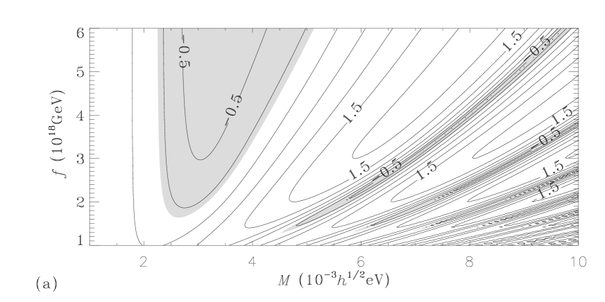
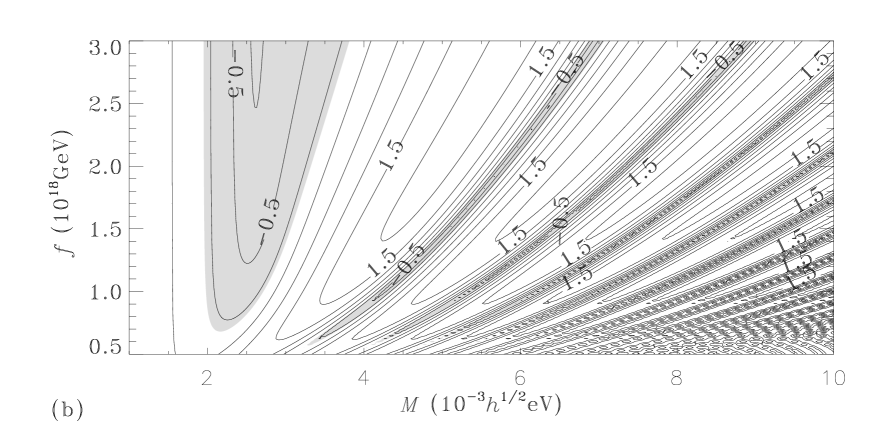
In Figs. 5 and 6 we display contour plots of $\Omega_{\phi 0}$ and $H_{0}t_{0}$ in the $M$,$f$ parameter space for two values $w_{i}=1.5$ and $w_{i}=0.5$. Similar figures have been given by Frieman and Waga [20] in the $w_{i}=1.5$ case, although our resolution is somewhat better. As $w_{i}$ decreases the contour plots do not change significantly in terms of their overall features, but contours with equivalent values shift to lower values of the $f$ parameter. For example, for large values of $M$ the $\Omega_{\phi 0}=0.7$ contour lies at a value $f\simeq 2.05\times 10^{18}\;\hbox{GeV}\;$ if $w_{i}=1.5$, while the same contour lies at $f\simeq 0.94\times 10^{18}\;\hbox{GeV}\;$ if $w_{i}=0.5$.

The other principal feature of the plots 5 and 6, which was not commented on in Ref. [20], is the wave-like properties of the contours at larger values of $M$. These features can be readily understood by considering the corresponding plots of the deceleration parameter, $q_{0}$, which is defined in terms of $u(t_{0})$, $v(t_{0})$, and $w(t_{0})$ by

$$q_{0} = {3\over 2}v^{3}(t_{0})+{1\over 2}u^{2}(t_{0})-1\ ,$$ (47)

$$= \frac{1}{2}\left(1+3\Omega_{\phi 0}-6{y_{0}}^{2}\right)\ .$$ (48)

We display contour plots of $q_{0}$ in the $M$,$f$ parameter space in Fig. 7. Essentially, as $M$ increases for roughly fixed $f$ for sufficiently large $M$, the value of $q_{0}$ oscillates over negative and positive values, from a minimum of $q_{0}=\frac{1}{2}\left(1-3\Omega_{\phi 0}\right)$ to a maximum $q_{0}=\frac{1}{2}\left(1+3\Omega_{\phi 0}\right)$ about a mean of $q_{0}=0.5$. This corresponds to the scalar field, $\phi$, having undergone more and more oscillations by the time of the present epoch. The minimum value of $q_{0}$ is attained when $\dot{\phi}=0$ instantaneously, while the maximum value of $q_{0}$ is attained when $\phi$ is instantaneously passing through the minimum of its potential.

For smaller values of $M$ to the left of the plots the scalar field has only relatively recently become dynamical, whereas for larger values of $M$, the scalar can already have undergone several oscillations by the time of the present epoch, particularly if $f$ is small. This variation can be understood in terms of the asymptotic period of oscillation of solutions which approach ${\rm C}_{1}$, which by Eqs. (30), (31) is

$$t_{a}=2\pi{\cal F}/m=2\pi f/M^{2}.$$ (49)

The period $t_{a}$ is shorter for larger $M$, or for smaller $f$. Since the final $f$ values plotted in the $w_{i}=0.5$ case are a factor of 2 smaller than the $w_{i}=1.5$ case, this also explains why points with the same value of $M$ have undergone more oscillations up to the present epoch for the smaller value of $w_{i}$.

The value of $H_{0}t_{0}$ oscillates as $M$ increases for roughly fixed $f$, according to whether the universe has been accelerating or decelerating in the most recent past, with more rapid variation for parameter values with shorter asymptotic periods, $t_{a}$.

The wiggles in the $\Omega_{\phi 0}$ contours are a residual effect of the oscillation of the scalar field as $\Omega_{\phi}$ settles down to a constant value according to (38). The variation in the value of $\Omega_{\phi 0}$ with the value of $w_{i}$ can be understood from the fact that for smaller values of $w_{i}$ the scalar field begins its evolution in the matter-dominated era closer to the critical points, ${\rm C}_{1+}$, corresponding to the maximum of the potential, $V(\phi)$. For fixed $M$ and $f$ the period of quasi-inflationary expansion is therefore longer, and the present value of $\Omega_{\phi 0}$ larger.

IV Constraints from High-redshift type IA Supernovae

Empirical calibration of the light curve - luminosity relationship of type Ia supernovae provides absolute magnitudes that can be used as distance indicators. Since the luminosity distance of a light source, $d_{L}$, is defined by

$${H_{0}d_{L}\over c}=(z+1)\int^{\tau_{0}}_{\tau}(z+1)\,d\tau,$$ (50)

with $\tau=H_{0}t$, it is convenient to define an additional variable

$$r=-\int^{\tau}_{\tau_{0}}v\,d\tau\ ,$$ (51)

which is proportional to the comoving coordinate distance

$$r_{\text{comoving}}={r\over H_{0}a(t_{0})v(t_{0})}\,.$$ (52)

We then adjoin a differential equation

$$r^{\prime}=-v$$ (53)

to the differential equations (39)-(41) when performing the numerical integration. In terms of $r$ and $v$, the luminosity distance is then determined according to

$${H_{0}d_{L}\over c}={v\over\Omega_{m0}^{2/3}}(r-r(t_{0}))\ ,$$ (54)

and can be used in the appropriate distance modulus to compare with the supernovae data.

Frieman and Waga [26] have recently considered constraints on PNGB models from supernovae data (without source evolution) using the data set of Riess et al. [6]. We will perform a similar analysis, but we will make use of the largest available data set, namely the 60 supernovae published by Perlmutter et al. [5] (hereafter P98). Of these, 18 low redshift SNe Ia were discovered and measured in the Calán-Tololo survey [33], and the Supernova Cosmology Project discovered 42 new SNe Ia at redshifts between 0.17 and 0.83. The peak magnitudes of the supernovae are corrected using the “stretch factor” light curve fitting method [5, 34]. This method is based on fitting a time-stretched version of a single standard template to the observed light curve. The stretch factor is then used to estimate the absolute magnitude.

A Models without evolution

FIG. 8.: Confidence limits on $M$,$f$ parameter values, with $w_{i}=1.5$ and no evolution of sources, for the 60 supernovae Ia in the P98 dataset. Parameter values excluded at the 95.4% level are darkly shaded, while those excluded at the 68.3% level are lightly shaded.

We use the stretch-luminosity corrected effective $B$-band peak magnitude in Table 1 of P98 as the absolute magnitude and denote it as $m^{\text{eff}}_{B}$. The distant modulus of a supernova is defined as $m^{\text{eff}}_{B}+{\cal M}_{0}$, where ${\cal M}_{0}$ is the fiducial absolute magnitude which has not been given in the literatures. A fitting method to obtain ${\cal M}_{0}$, using only the 18 Calán/Tololo supernovae, can be found in [35, 36]. Perlmutter et al.[5] calculate the confidence regions by simply integrating over ${\cal M}_{0}$. In this paper, we will perform an analytic marginalization over ${\cal M}_{0}$ and obtain the marginal likelihood.

Similarly to the $\chi^{2}$ statistic used by Riess et al. [6], we define the quadratic form

$$\chi^{2}(M,f)=\sum^{60}_{i=1}{(m^{\text{eff}}_{B,i}+{\cal M}_{0}-\mu_{i})^{2}\over\sigma_{i}^{2}}$$ (55)

where $\mu_{i}(z_{i};H_{0},M,f)$ is the predicted distance modulus for model parameters $(M,f)$, and

$$\sigma_{i}^{2}=\sigma^{2}_{m^{\text{eff}}_{B,i}}+\left({5\log{\rm e}\over z_{i}}\sigma_{z,i}\right)^{2}\ .$$ (56)

The predicted distance modulus is

$$\mu_{i}=5\log{d_{L}(z_{i})}+25\ ,$$ (57)

if the luminosity distance, $d_{L}$, as defined by (50) or (54), is given in units of Megaparsecs.

In order to perform analytic marginalization over $H_{0}$ as well as over ${\cal M}_{0}$ we separate out the $H_{0}$ and ${\cal M}_{0}$ dependence from $\mu_{i}$ into a quantity, $\nu$, which we define by

$$\mu_{i}-{\cal M}_{0}=g_{i}+\nu$$ (58)

where $g_{i}(z_{i};M,f)$ depends implicitly only on $M$ and $f$. We then follow the statistical procedures adopted by Drell, Loredo and Wasserman [37, 38] and marginalize over $\nu$ using a flat prior that is bounded over some range $\Delta\nu$.

The marginal likelihood is

$${\cal L}(M,f)={1\over\Delta\nu}\int{d\nu\;{\rm e}^{-\chi^{2}/2}}={s\sqrt{2\pi}\over\Delta\nu}{\rm e}^{-Q/2}\$$ (59)

where

$$Q(M,f)=\sum^{60}_{i=1}{(m^{\text{eff}}_{B,i}-g_{i}-\hat{\nu})^{2}\over\sigma_{i}^{2}}$$ (60)

and $\hat{\nu}(M,f)$ is the best-fit value of $\nu$ given $M$ and $f$, with conditional uncertainty $s$. We identify $1/s^{2}$ as the coefficient of $\nu^{2}$ in (55),

$${1\over s^{2}}=\sum^{60}_{i=1}{1\over\sigma_{i}^{2}}\ ,$$ (61)

and $\hat{\nu}$ as $s^{2}$ times the coefficient of $-\nu$, viz.

$$\hat{\nu}(M,f)=s^{2}\sum^{60}_{i=1}{m^{\text{eff}}_{B,i}-g_{i}\over\ \sigma_{i}^{2}}\ .$$ (62)

The quadratic form (60) is what one would obtain by calculating the “maximum likelihood” for $M$ and $f$. Since $s$ is independent of $M$ and $f$, it follows from Eq. (59) that the marginal likelihood is proportional to the maximum likelihood in this case.

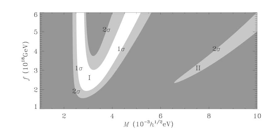
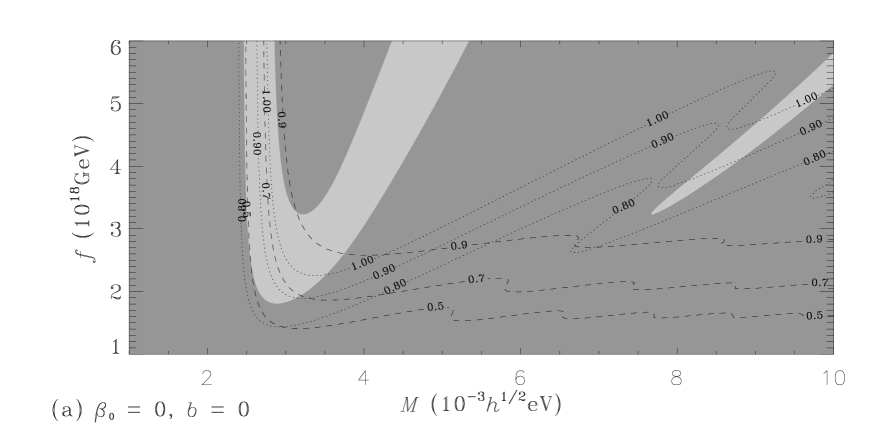
Fig. 8 shows the 68.3% and 95.4% joint credible regions for $M$ and $f$, and is a direct analogue of Fig. 1 of Ref. [26], where a similar analysis was performed on 37 supernovae given in R98. The position of the region of parameters which are included at both the 68.3% and 95.4% confidence levels is broadly similar to that obtained from the R98 data [26]. Although Frieman and Waga [26] did not include the parameter region $M>0.004h\;\hbox{eV}\;$, we have redone their analysis on the R98 data and find that the parameter values to the right of Fig. 8 which are admitted at the 95.4% level but excluded at the 68.3% level for the P98 dataset, (labelled region II in Fig. 8), are in fact excluded also at the 95.4% confidence level if the 37 supernovae of the R98 dataset are used. It is possible that this discrepancy has its origin in the different techniques used by Riess et al. [6] to determine the distance moduli. Possible systematic discrepancies in the “stretch factor” method of P98 versus the “multi-colour light curve” and “template fitting methods” of R98 have been discussed in some detail in Ref. [37].

The importance of the $2\sigma$ included parameter region to right of Fig. 8 diminishes, however, if one compares it with Figs. 5 and 6, since it largely corresponds to parameter values with $\Omega_{\phi 0}\mathop{\hbox{${\lower 3.8pt\hbox{$>$}}\atop{\raise 0.2pt\hbox{$\sim$}}$}}0.9$, which can be discounted by dynamical measurements of $\Omega_{m0}$, where $\Omega_{m0}+\Omega_{\phi 0}=1$. Furthermore, the few allowed values below the $\Omega_{\phi 0}=0.9$ contour in this part of the parameter space have unacceptably small values for the age of the Universe, $H_{0}t_{0}$.

The parameter region $0.002h\;\hbox{eV}\;<M<0.003h\;\hbox{eV}\;$ which from Fig. 8 is admitted at both the 68.3% and 95.4% levels, (labelled region I), by contrast, corresponds to acceptable values of both $\Omega_{\phi 0}$ and $H_{0}t_{0}$. Comparing with Fig. 7, we see that this region has $-0.1\mathop{\hbox{${\lower 3.8pt\hbox{$<$}}\atop{\raise 0.2pt\hbox{$\sim$}}$}}q_{0}\mathop{\hbox{${\lower 3.8pt\hbox{$<$}}\atop{\raise 0.2pt\hbox{$\sim$}}$}}-0.6$, corresponding to a Universe with a scalar field still in an early stage of rolling down the potential $V(\phi)$. The label I is thus indicative of the fact that the scalar field is rolling down the potential for the first time (from left to right), while in region II the scalar field is rolling down the potential for the second time (from right to left). In region II $q_{0}$ is positive – however, it corresponds to parameter values for which there would have been a cosmological acceleration at modest redshifts in the past, e.g., at $z\mathop{\sim}\limits 0.2$, well within the range of the current supernovae dataset.

Since conclusions regarding statistically preferred regions of the parameter space can change if evolution of the sources occurs, we think it is important that this possibility is also examined, as we will now do.

B Models with evolution

FIG. 9.: Confidence limits on $M$,$f$ parameter values in the best-fit $\beta_{0}=0.414$ slice of the $(M,f,\beta_{0})$ parameter space, with $w_{i}=1.5$, for the 60 supernovae Ia in the P98 dataset. Parameter values excluded at the 95.4% level are darkly shaded, while those excluded at the 68.3% level are lightly shaded. For reference, contours of $\Omega_{\phi 0}$ and $H_{0}t_{0}$ are superposed as dashed and dotted lines respectively.

FIG. 10.: Confidence limits on $M$,$f$ parameter values in the $\beta_{0}=0$ slice of the $(M,f,\beta_{0})$ parameter space relative to a best-fit value $\beta^{*}\simeq 0.414$, for the 60 supernovae Ia in the P98 dataset, with $w_{i}=1.5$. Parameter values excluded at the 95.4% level are darkly shaded, while those excluded at the 68.3% level are lightly shaded. For reference, contours of $\Omega_{\phi 0}$ and $H_{0}t_{0}$ are superposed as dashed and dotted lines respectively.

FIG. 11.: Confidence limits on $M$,$f$ parameter values in the $\beta_{0}=0$ slice of the $(M,f,\beta_{0})$ parameter space relative to a best-fit value $\beta^{*}\simeq 0.435$, for the 60 supernovae Ia in the P98 dataset, with $w_{i}=0.2$. Parameter values excluded at the 95.4% level are darkly shaded, while those excluded at the 68.3% level are lightly shaded. For reference, contours of $\Omega_{\phi 0}$ and $H_{0}t_{0}$ are superposed as dashed and dotted lines respectively.

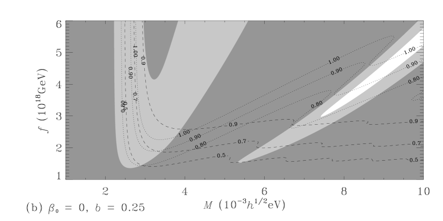
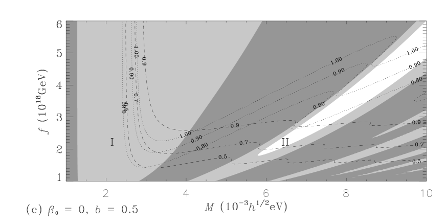
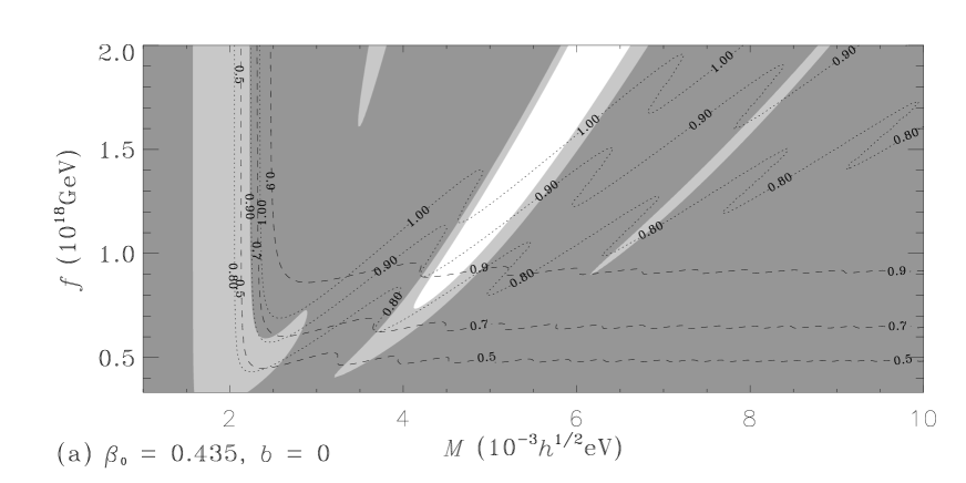
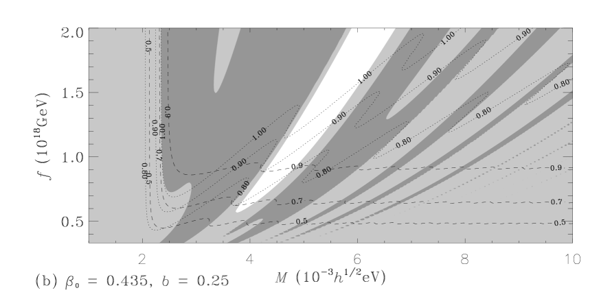
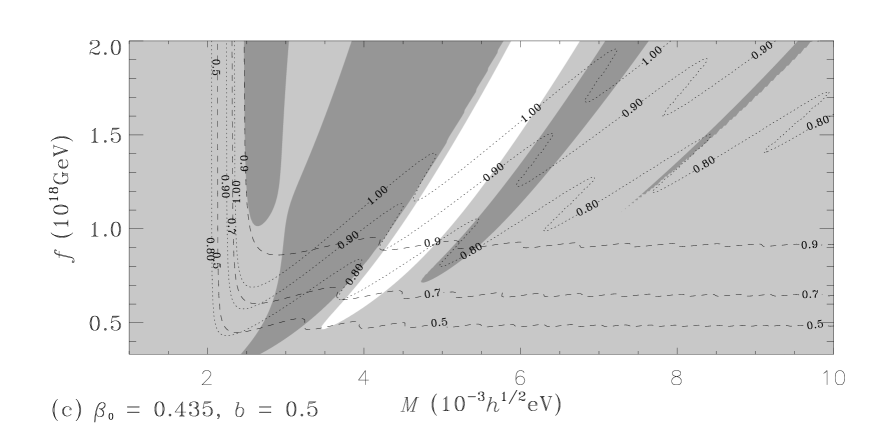
In view of the recent results of Refs. [7, 8], supernovae Ia may exhibit some evolutionary behaviour, at least as far as their rise times are concerned. A possible evolution in the peak luminosity is therefore a possibility which must be seriously investigated.

In the absence of a detailed physical model to explain precisely how the source peak luminosities vary with redshift, one approach is to assume some particular empirical form for the source evolution, and to examine the consequences. Such an analysis has been recently preformed by Drell, Loredo and Wasserman [37] in the case of Friedmann-Lemaître models with constant vacuum energy. We will undertake an equivalent analysis for the case of PNGB quintessential cosmologies.

Following Drell, Loredo and Wasserman [37] we will assume that the intrinsic luminosities of SNe Ia scale as a power of $1+z$ as a result of evolution. This model introduces a continuous magnitude shift of the form $\beta\ln(1+z)$ to the SNe Ia sample. Eq. (55) then becomes

$$\chi^{2}(M,f)=\sum^{60}_{i=1}{(m^{\text{eff}}_{B,i}-g_{i}-\nu-\beta\ln(1+z_{i}))^{2}\over\sigma_{i}^{2}}\ .$$ (63)

The parameter $\beta$ will be assumed to have a Gaussian prior distribution with mean $\beta_{0}$ and standard deviation $b$. Physically the parameter $\beta_{0}$ represents a redshift-dependent evolution of the peak luminosity of the supernovae sources, which might be expected to arise as a result of the chemical evolution of the environment of the supernovae progenitors as abundances of heavier elements increase with cosmic time. Ultimately, one should hope to account for this evolution with astrophysical modelling of the supernovae explosions [9]. The parameter $b$ would then account for a local variability in the supernovae environments between regions of individual galaxies at the same redshift which are richer or poorer in metals, or with progenitor populations of different ages and masses etc.

We now have two parameters to marginalize over, $\nu$ and $\beta$. As in the case of models with no evolution, we will marginalize over $\nu$ using a flat prior. We use a Gaussian prior for $\beta$ with mean $\beta_{0}$ and standard deviation $b$, so that

$$p(\beta^{\prime})={1\over b\sqrt{2\pi}}{\rm e}^{-\beta^{\prime 2}/2b^{2}}$$ (64)

where

$$\beta^{\prime}=\beta-\beta_{0}\ .$$ (65)

The marginal likelihood is calculated by multiplying the prior (64) by the likelihood resulting from Eq. (59), and integrating over $\beta$. The resulting likelihood is

$${\cal L}(M,f) = {1\over\Delta\nu}\int{d\beta^{\prime}\;\int{d\nu\;p(\beta^{\prime}){\rm e}^{-\chi^{2}/2}}}$$ (66)

$$= {s{\bar{\sigma}}\sqrt{2\pi}\over\Delta\nu b}{\rm e}^{-Q/2}$$ (67)

where

$$Q(M,f) = -{\hat{\beta}^{2}\over{\bar{\sigma}}^{2}}+\sum^{60}_{i=1}{(h_{i}-s^{2}{\cal H})^{2}\over\sigma_{i}^{2}}\ ,$$ (68)

$$h_{i}(z_{i};M,f) = m^{\text{eff}}_{B,i}-g_{i}-\beta_{0}\ln(1+z_{i})\ ,$$ (69)

$${\cal H}(M,f) = \sum^{60}_{i=1}{h_{i}\over\sigma_{i}^{2}}\ .$$ (70)

The conditional best-fit of $\beta^{\prime}$ is given by

$$\hat{\beta}(M,f) = {\bar{\sigma}}^{2}\sum^{60}_{i=1}{h_{i}[\ln(1+z_{i})-s^{2}{\cal G}]\over\sigma_{i}^{2}}\ ,$$ (71)

$${\cal G} = \sum^{60}_{i=1}{\ln(1+z_{i})\over\sigma_{i}^{2}}\ ,$$ (72)

and the $\beta^{\prime}$ uncertainity, ${\bar{\sigma}}$, is given by

$${1\over{\bar{\sigma}}^{2}}={1\over b^{2}}-s^{2}{\cal G}^{2}+\sum^{60}_{i=1}{\ln^{2}(1+z_{i})\over\sigma_{i}^{2}}\ .$$ (73)

Although ${\bar{\sigma}}$ is independent of $M$ and $f$, the marginal likelihood is no longer proportional to the profile likelihood because $Q$ is now given by (68) rather than by the chi-square type statistic (60).

We have performed a detailed numerical analysis on the P98 dataset, varying $\beta_{0}$, $b$ and $w_{i}$. As a result we find a best-fit value of $\beta_{0}\equiv\beta^{*}\simeq 0.414$, for $w_{i}=1.5$ in the PNGB models. This would correspond to supernovae being intrinsically dimmer by $0.17$ magnitudes at a redshift of $z=0.5$, which is an effect of the typical order of magnitude being addressed in current attempts to better model the supernova explosions [9]. Furthermore, we find that inclusion of a non-zero variance, $b^{2}$, does not alter the prediction of the best-fit value of $\beta_{0}$, although it naturally does lead to a broadening of the areas of parameter space included at the $2\sigma$ level. There is relatively little broadening of the region of parameter values included at the $1\sigma$ level in the $\beta_{0}=\beta^{*}$ plane, however, which is no doubt a consequence of the steepness of the $q_{0}$ contours in Fig. 7(a) in the area corresponding to region II.

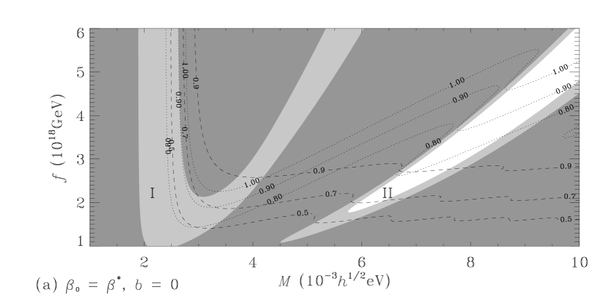
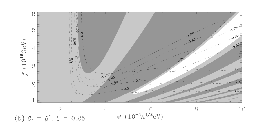
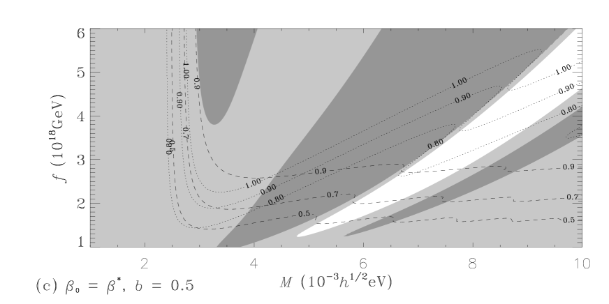
In Figs. 9 and 10 we display the joint credible regions for $M$ and $f$, for two slices through the 3-dimensional $(M,f,\beta_{0})$ parameter space for $w_{i}=1.5$: (a) the best-fit case $\beta_{0}=\beta^{*}$; and (b) $\beta_{0}=0$. Analogously, the best-fit case is shown in Fig. 11 for $w_{i}=0.2$. We see from Fig. 10 that once the likelihood is normalized relative to $\beta^{*}$ no regions remain in the $\beta=0$ parameter plane which are admitted at the $1\sigma$ level when $b=0$. Furthermore, even when a non-zero standard deviation, $b$, is included, region II of the $(M,f)$ parameter plane is favoured at the $1\sigma$ level, in contrast to Fig. 8.

We have also undertaken an analysis of the models with $\beta_{0}=0$ but variable $b$, similarly to the study of Ref. [37]. In that case, we once again find that region II of the $(M,f)$ parameter plane is admitted at the $1\sigma$ level if $b=0.25$ or $b=0.5$. The dependence of the value of

$$\bar{Q}\equiv-2\ln\left({\cal L}\Delta\nu\right)=Q-2\ln\left(\sqrt{2\pi}\,s{\bar{\sigma}}\over b\right)$$ (74)

on the value of $b$ is displayed in Fig. 12, for $\beta_{0}=0$ as compared with the best-fit case $\beta_{0}=\beta^{*}$. The quantity $\bar{Q}$ is analagous to the chi-square statistic of the maximum likelihood method. We see that the $\beta_{0}=0$ models favour a non-zero value of $b\simeq 0.36$ by a very small margin as compared to the $b=0$ case. For $b=0.36$ the points of greatest likelihood lie mainly in region II, in contrast to the $b=0$ case in Fig. 8.

FIG. 12.: Variation of the least value of $\bar{Q}=-2\ln\left({\cal L}\Delta\nu\right)$ as a function of the standard deviation $b$ of the prior distribution for $\beta_{0}$ for values $\beta_{0}=0$ and $\beta_{0}=\beta^{*}$.

Varying the inital condition $w_{i}$ does not appear to affect the best-fit value of $\beta_{0}$ significantly. For $w_{i}=0.2$ (cf.,Fig. 11), for example, the best-fit value was $\beta^{*}=0.435$, a difference of 5% from the $w_{i}=1.5$ case. Furthermore, the numerical value of the least value of $\bar{Q}$ was only 0.2% greater in the $w_{i}=0.2$ case. We have not attempted to find a best-fit value for $w_{i}$.

V Constraints from Lensing Statistics

FIG. 13.: Confidence limits from gravitational lensing statistics: (a) $w_{i}=1.5$; (b) $w_{i}=0.2$. Parameter values excluded at the 95.4% level are darkly shaded, while those excluded at the 68.3% level are lightly shaded. For reference, contours of $\Omega_{\phi 0}$ and $H_{0}t_{0}$ are superposed as dashed and dotted lines respectively.

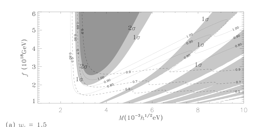
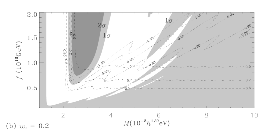
Gravitational lensing of distant light sources due to the accumulation of matter along the line of sight provide another relatively sensitive constraint on the cosmological models of interest. For cosmology the situation of most interest is the lensing of high luminosity quasars by intervening galaxies. The abundance of multiply imaged quasars and the observed separation of the images to the source puts constraint on the luminosity–redshift relation and hence the model parameters. Basically, if the volume of space to a given redshift is larger then on average one can expect more lensing events. This leads to a statistical test, which has been used to put bounds on $\Lambda$ [27, 28, 29] and to test properties of some decaying $\Lambda$ or quintessence models [32, 39].

Gravitational lensing statistics are useful since they provide a tests which potentially provides opposing constraints to those obtained from supernovae magnitude–redshift tests. In particular, in the case of models with a vacuum energy provided by a cosmological constant, the high redshift supernovae have been interpreted as favouring relatively large values of $\Omega_{\Lambda}$ - Perlmutter et al. [5] give a value of $\Omega_{\Lambda}=0.72$ at $1\sigma$ level - whereas the gravitational lensing data leads to upper bounds on $\Omega_{\Lambda}$: Kochanek [27] quotes $\Omega_{\Lambda}<0.66$ at the $2\sigma$ level. A combined likelihood analysis has been performed by various authors [26, 29, 32].

Gravitational lensing constraints on the PNGB models have been very recently given by Frieman and Waga [26] for $w_{i}=1.5$. However, Frieman and Waga considered a more retricted range of parameter space, $M<0.005h\;\hbox{eV}\;$, since they did not consider the possibility of source evolution in the case of the type Ia supernovae and therefore took values of $M>0.005h\;\hbox{eV}\;$ to be ruled out. We wish to extend the range of $M$ for the gravitational lensing statistcs to consider parameter values corresponding to region II in the supernovae constraint graphs, Figs. 8, 10, so as to compare the constraints from different tests.

We have thus simply followed the calculation described by Waga and Miceli [32], who performed a statistical lensing analysis of optical sources described earlier by Kochanek [27]. They used a total of 862 ($z>1$) high luminosity quasars plus 5 lenses from seven major optical surveys [40]. (Another alternative not considered here is to analyse data from radio surveys – see, e.g., [28, 29].) Undertaking a similar analysis for the increased parameter range, we arrive at Fig. 13, which shows the 68.3% and 95.4% joint credible regions for $M$ and $f$, for two values of $w_{i}$. We refer the reader to Refs. [27, 32] for details of the calculation. The only regions of parameter space excluded at the $2\sigma$ level turn out to be areas of parameter space for which the deceleration is presently negative (cf., Fig. 7), with the scalar field still commencing its first oscillation at the present epoch.

VI Discussion

Let us now consider the overall implications of the constraints observed above.

Firstly, since empirical models with source evolution do appear to fit the data somewhat better, it would appear that we do have weak evidence for an underlying evolution of the peak luminosity of the type Ia supernovae sources, at least in the context of the PNGB quintessence models. It might be interesting to compare the case of other quintessence models, or the case of a cosmological constant. However, the PNGB model is qualitatively different from such models since its final state corresponds to one in which the ultimate destiny of the universe is to expand at the same rate as a spatially flat Friedmann–Robertson–Walker model, rather than to undergo an accelerated expansion. This is of course precisely why we chose the PNGB models as the basis of our investigation, rather than models in which a late–time accelerated expansion had been built in by hand. If we wish to test the hypothesis that the faintness of the type Ia supernovae is at least partly due to an intrinsic variation of their peak luminosities – which is a very real possibility in view of the results of [7] – then a quintessence model which possesses a variety of possibilities for the present–day variation of the scale factor is probably the best type of model to investigate.

If only supernovae luminosity distances, (cf., Fig. 9, and gravitational lensing statistics, (cf., Fig. 13), are compared then we see that there is a remarkable concordance between the two tests – region II of Fig. 9 coincides with a region included at even the $1\sigma$ level in Fig. 13. This is perhaps not surprising, since in view of Fig. 7 region II corresponds to parameter values for which the present day universe has already undergone almost one complete oscillation of the scalar field about the final critical point ${\rm C}_{2}$ of Fig. 1. It is thus already well on the way towards its asymptotic behaviour, which closely resembles that of a standard spatially flat Friedmann-Robertson-Walker model.

Due to the oscillatory behaviour, parameter values in region II correspond to models in which there has been a recent cosmological acceleration, (e.g., at $z\mathop{\sim}\limits 0.2$), but with a $q(z)$ which changes sign three times over the larger range of redshifts, $0<z<4$, in the quasar lensing sample, and therefore differing significantly from Friedmann–Lemaître models over this larger redshift range. Extending the SNe Ia sample to include objects at redshifts $0.1<z<0.4$ and $z>0.85$ in substantial numbers would greatly improve the ability to decide between models in regions I and II.

There is some cause for concern, however, if we consider the favoured values of $\Omega_{\phi 0}$ and $H_{0}t_{0}$. In the case of the models with empirical evolution of the supernovae sources, we always found that the best-fit parameter values occured at the $\Omega_{\phi 0}\rightarrow 1$ boundary of the ($M,f$) parameter space. The overwhelming evidence of many astronomical observations over the past two decades [41] would tend to indicate that $\Omega_{m0}\simeq 0.2\pm 0.1$, indicating that a vacuum energy fraction of $\Omega_{\phi 0}\mathop{\sim}\limits 0.7$–$0.8$ is desirable, and $\Omega_{\phi 0}\mathop{\hbox{${\lower 3.8pt\hbox{$<$}}\atop{\raise 0.2pt\hbox{$\sim$}}$}}0.9$ in any case. Although parameter values with $\Omega_{\phi 0}<0.8$ certainly fall within both the 2$\sigma$ and 1$\sigma$ portions of region II of Fig. 9, for all values of $b$, there are potentially serious problems if we wish to simultaneously obtain large values of $H_{0}t_{0}$. In view of recent estimates of the ages of globular clusters [42], a lower bound of 12 Gyr for the age of the Universe appears to currently indicated. With $h\simeq 0.65$ this would require $H_{0}t_{0}\mathop{\hbox{${\lower 3.8pt\hbox{$>$}}\atop{\raise 0.2pt\hbox{$\sim$}}$}}0.8$. For $w_{i}=1.5$, parameter values with $H_{0}t_{0}>0.8$ coincide with values $\Omega_{\phi 0}\mathop{\hbox{${\lower 3.8pt\hbox{$>$}}\atop{\raise 0.2pt\hbox{$\sim$}}$}}0.9$ in region II, which is phenomenologically problematic.

The tension between the values of $\Omega_{\phi 0}$ and $H_{0}t_{0}$ is somewhat mitigated for lower values of $w_{i}$. For $w_{i}=0.2$, for example, we see from Figs. 11 and 13(b) that the $\Omega_{\phi 0}=0.7$ and $H_{0}t_{0}$ meet in Region II, and there is a small region of parameters there with $0.7\mathop{\hbox{${\lower 3.8pt\hbox{$<$}}\atop{\raise 0.2pt\hbox{$\sim$}}$}}\Omega_{\phi 0}\mathop{\hbox{${\lower 3.8pt\hbox{$<$}}\atop{\raise 0.2pt\hbox{$\sim$}}$}}0.9$ and $H_{0}t_{0}\mathop{\hbox{${\lower 3.8pt\hbox{$>$}}\atop{\raise 0.2pt\hbox{$\sim$}}$}}0.8$, which is also consistent with the other cosmological tests.

Even if the supernovae sources undergo evolution it is clear that parameter values in region I of 8 which are favoured in the absence of evolution of peak SnIa luminosities, are still included at the $2\sigma$ level in the models with evolution, in view of Fig. 9.

Perhaps the most significant aspect of our results is the fact that the mere introduction of an additional dispersion, $b>0.17$, in the peak luminosities while leaving their mean value fixed (cf., Fig. 12), gives rise to a change in the best-fit region of parameter space from region I to region II. (See [43] for further details.) One would imagine that an increased dispersion is likely to be a feature of many models of source evolution, even if evolutionary effects are of secondary importance. Thus even if the empirical models with non-zero $\beta$ are somewhat artificial, more sophisticated scenarios could well lead to similar changes in regard to the fitting of cosmological parameters in the PNGB model.

Much tighter bounds on the parameter space of quintessence models, including the present model, will be obtained over the next decade as more supernovae data is collected. What we wish to emphasize, however, is that an effective vacuum energy which is cosmologically significant at the present epoch should not simply be thought of in terms of a “cosmic acceleration”. A dynamical vacuum energy with a varying effective equation of state allows for many possibilities for the evolution of the universe, and overly restrictive assumptions, such as equating quintessence to models with a late period of continuous cosmological acceleration, should be avoided. If detailed astrophysical modeling of type Ia supernovae explosions ultimately shows that the dimness of distant supernova events is largely due to evolutionary effects, it does not spell the end for cosmologies with dynamical scalar fields.

REFERENCES

- [1] Electronic address: cng@physics.adelaide.edu.au
- [2] Electronic address: dlw@physics.adelaide.edu.au
- [3] R.R. Caldwell, R. Dave and P.J. Steinhardt, Phys. Rev. Lett. 80, 1582 (1998); G. Huey, L. Wang, R. Dave, R.R. Caldwell and P.J. Steinhardt, Phys. Rev. D59, 063005 (1999).
- [4] S. Perlmutter et al., Nature 391, 51 (1998); B.P. Schmidt et al., Astrophys. J. 507, 46 (1998).
- [5] S. Perlmutter et al., Astrophys. J. 517, 565 (1999).
- [6] A.G. Riess et al., Astron. J. 116, 1009 (1998).
- [7] A.G. Riess, A.V. Filippenko, W. Li and B.P. Schmidt, Astron. J. 118, 2668 (1999).
- [8] G. Aldering, R. Knop and P. Nugent, Astron. J. 119, 2110 (2000).
- [9] D. Arnett, astro-ph/9908169 (1999); P. Höflich, K. Nomoto, H. Umeda and J.C. Wheeler, Astrophys. J. 528, 590 (2000).
- [10] A.G. Riess et al., Astron. J. 118, 2675 (1999).
- [11] P. Steinhardt, in Critical Problems in Physics, eds. V.L. Fitch and D.R. Marlow (Princeton Univ. Press, 1997).
- [12] A.R. Liddle and R.J. Scherrer, Phys. Rev. D59, 023509 (1999).
- [13] P.J.E. Peebles and B. Ratra, Astrophys. J. 325, L17 (1988); Phys. Rev. D37, 3406 (1988).
- [14] I. Zlatev, L. Wang and P.J. Steinhardt, Phys. Rev. Lett. 82, 896 (1999); P.J. Steinhardt, L. Wang and I. Zlatev, Phys. Rev. D59, 123504 (1999); I. Zlatev and P.J. Steinhardt, Phys. Lett. B459, 570 (1999).
- [15] F. Lucchin and S. Matarrese, Phys. Rev. D32, 1316 (1985); Y. Kitada and K. Maeda, Class. Quantum Grav. 10, 703 (1993).
- [16] J.J. Halliwell, Phys. Lett. B185, 341 (1987); C. Wetterich, Nucl. Phys. B302, 668 (1988); A.B. Burd and J.D. Barrow, Nucl. Phys. B308, 929 (1988); A.A. Coley, J. Ibañez and R.J. van den Hoogen, J. Math. Phys. 38, 5256 (1997); P.G. Ferreira and M. Joyce, Phys. Rev. D58, 023503 (1998); S.C.C. Ng, Phys. Lett. B485, 1 (2000).
- [17] D. Wands, E.J. Copeland and A.R. Liddle, Ann. N.Y. Acad. Sci. 688, 647 (1993).
- [18] P.G. Ferreira and M. Joyce, Phys. Rev. Lett. 79, 4740 (1997).
- [19] P.T.P. Viana and A.R. Liddle, Phys. Rev. D57, 674 (1998).
- [20] J.A. Frieman and I. Waga, Phys. Rev. D57, 4642 (1998).
- [21] E.J. Copeland, A.R. Liddle and D. Wands, Phys. Rev. D57, 4686 (1998).
- [22] A. de la Macorra and G. Piccinelli, hep-ph/9909459.
- [23] C.T. Hill and G.G. Ross, Nucl. Phys. B311, 253 (1988); Phys. Lett. B203, 125 (1988).
- [24] J.A. Frieman, C.T. Hill, A. Stebbins and I. Waga, Phys. Rev. Lett. 75, 2077 (1995).
- [25] K. Coble, S. Dodelson and J.A. Frieman, Phys. Rev. D55, 1851 (1997).
- [26] I. Waga and J.A. Frieman, Phys. Rev. D62, 043521 (2000).
- [27] C.S. Kochanek, Astrophys. J. 466, 638 (1996).
- [28] E.E. Falco, C.S. Kochanek and J.A. Muñoz, Astrophys. J. 494, 47 (1998).
- [29] P. Helbig, Astron. Astrophys. 350, 1 (1999).
- [30] K. Freese, J.A. Frieman and A.V. Olinto, Phys. Rev. Lett. 65, 3233 (1990); F.C. Adams, J.R. Bond, K. Freese, J.A. Frieman and A.V. Olinto, Phys. Rev. D47, 426 (1993).
- [31] V.A. Belinsky, I.M. Khalatnikov, L.P. Grishchuk and Ya.B. Zeldovich, Sov. Phys. JETP 62, 195 (1985) [Zh. Eksp. Teor. Fiz. 89, 346 (1985)]; D.L. Wiltshire, Phys. Rev. D36, 1634 (1987).
- [32] I. Waga and A.P.M.R. Miceli, Phys. Rev. D59, 103507 (1999).
- [33] M. Hamuy et al., Astron. J. 112, 2408 (1996).
- [34] S. Perlmutter et al., Astrophys. J. 483, 565 (1997).
- [35] M. Hamuy, M.M. Philips, J. Maza, N.B. Suntzeff, R.A. Schommer and R. Aviles, Astron. J. 109, 1 (1995).
- [36] M. Hamuy, M.M. Philips, R.A. Schommer, N.B. Suntzeff, J. Maza and R. Aviles, Astron. J. 112, 2391 (1996).
- [37] P.S. Drell, T.J. Loredo and I. Wasserman, Astrophys. J. 530, 593 (2000).
- [38] Our quantity is identical to the quantity given in Appendix B of [37].
- [39] B. Ratra and A. Quillen, Mon. Not. Roy. Astron. Soc. 259, 738 (1992); L.F. Bloomfield Torres and I. Waga, Mon. Not. Roy. Astron. Soc. 279, 712 (1996); V. Silveira and I. Waga, Phys. Rev. D56, 4625 (1997); A.R. Cooray and D. Huterer, Astrophys. J. 513, L95 (1999).
- [40] D. Maoz et al., Astrophys. J. 409, 28 (1993); D. Crampton, R.D. McClure and J.M. Fletcher, Astrophys. J. 392, 23 (1992); H.K.C. Yee, A.V. Filipenko and D.H. Tang, Astron. J. 105, 7 (1993); J. Surdej et al., Astron. J. 105, 2064 (1993); E.E. Falco, in Gravitational Lenses in the Universe, eds. J. Surdej, D. Fraipont-Caro, E. Gosset, S. Refsdal and M. Remy (Univ. Liège, Liège, 1994), p. 127; C.S. Kochanek, E.E. Falco and R. Shild, Astrophys. J. 452, 109 (1995); A.O. Jaunsen, M. Jablonski, B.R. Pettersen and R. Stabell, Astron. Astrophys. 300, 323 (1995).
- [41] See, for example, J.P. Ostriker and P.J. Steinhardt, Nature 377, 600 (1995), and references therein.
- [42] L.M. Krauss, Phys. Rep. 333, 33 (2000).
- [43] D.L. Wiltshire, astro-ph/0010443 (2000).