The Bispectrum: From Theory to Observations

Abstract

The bispectrum is the lowest-order statistic sensitive to the shape of structures generated by gravitational instability and is a potentially powerful probe of galaxy biasing and the Gaussianity of primordial fluctuations. Although the evolution of the bispectrum is well understood theoretically from non-linear perturbation theory and numerical simulations, applications to galaxy surveys require a number of issues to be addressed. In this paper we consider the effect on the bispectrum of stochastic non-linear biasing, radial redshift distortions, non-Gaussian initial conditions, survey geometry and sampling.

We find that: 1) bias stochasticity does not affect the use of the bispectrum to recover the mean biasing relation between galaxies and mass, at least for models in which the scatter is uncorrelated at large scales. 2) radial redshift distortions do not change significantly the monopole power spectrum and bispectrum compared to their plane-parallel values. 3) survey geometry leads to finite-volume effects which must be taken into account in current surveys before comparison with theoretical predictions can be made. 4) sparse sampling and survey geometry correlate different triangles leading to a breakdown of the Gaussian likelihood approximation.

We develop a likelihood analysis using bispectrum eigenmodes, calculated by Monte Carlo realizations of mock surveys generated with second-order Lagrangian perturbation theory and checked against N-body simulations. In a companion paper we apply these results to the analysis of the bispectrum of IRAS galaxies.

1 Introduction

It is widely accepted that the large-scale structure of the universe routinely observed in galaxy surveys is the result of gravitational instability that operates on (initially small) fluctuations in the density distribution. Essentially, initially dense (underdense) regions contract (expand) as a consequence of the attractive nature of gravity. As a result, most of the volume of the universe is in underdense regions whereas the rest contains dense structures such as clusters, galaxies, etc. This asymmetry between underdense and overdense regions implies non-Gaussianity in the galaxy distribution. Understanding the dynamics of gravitational instability thus gives us a powerful tool that can be used to extract useful information from the non-Gaussian clustering pattern of galaxies (Peebles 1980; Fry 1984; Goroff et al. 1986; Bernardeau 1992; Bouchet et al. 1995; Scoccimarro & Frieman 1996).

A quantitative description of galaxy clustering is obtained by applying statistical methods, in particular, multi-point correlation functions (Peebles 1980). In a Gaussian field, the statistical properties are fully characterized by its two-point correlation function or power spectrum, all higher-order (connected) correlation functions being zero. Information on non-Gaussianity is thus accessible by calculating higher-order correlations functions. An alternative to multi-point correlation functions is to consider higher-order moments (i.e. smoothed multi-point correlation functions collapsed at a single point); these characterize the one-point distribution of the galaxy distribution and can be measured with larger signal to noise than the corresponding multi-point functions. However, the latter contain more information, in particular, being evaluated at three or more points they are sensitive to the shapes of large-scale structures, which is the key to disentangle degeneracies present otherwise.

The bispectrum, the three-point correlation function in Fourier space, is the lowest order statistic sensitive to the shape of structures generated by gravitational instability. It can be used to probe the nature of primordial fluctuations (Gaussian versus non-Gaussian), galaxy biasing (i.e. the relation between the galaxy distribution and the underlying dark matter distribution), and help to break the degeneracy between linear bias and the matter density parameter $\Omega_{m}$ present in power spectrum measurements in galaxy redshift surveys (Fry 1994; Hivon et al. 1995; Matarrese, Verde & Heavens 1997; Scoccimarro et al. 1998).

Pioneering work on three-point statistics from the Zwicky (Peebles & Groth 1975) and Lick (Groth & Peebles 1977; Fry & Seldner 1982) angular catalogs showed that the bispectrum, $B(k_{1},k_{2},k_{3})$, scaled in terms of the power spectrum, $P(k)$, as $B(k)\propto P(k)^{2}$. This motivatied the so-called hierarchical model and was also in agreement with the scaling at small scales inferred from the BBGKY equations of motion assuming stable clustering and self-similarity (Davis & Peebles 1977; Peebles 1980). At these small scales deep into the non-linear regime, however, limited understanding of the non-linear physics including the possibility of complicated galaxy biasing prevents using higher-order statistics to extract quantitative knowledge.

It was not until somewhat later, with the systematic development of non-linear perturbation theory (hereafter PT; Fry 1984), that it was possible to derive quantitatively how non-Gaussianity is generated by gravity. In particular, the scaling $B(k)\propto P(k)^{2}$ (and in general, the $n$-point function $\xi_{n}$ scales as $\xi_{n}\propto\xi_{2}^{n-1}$) is recovered at large scales, being simply a result of quadratic non-linearities in the equations of motion of gravitational instability. An important signature predicted by PT is that the bispectrum at large scales should be a rather strong function of triangle configuration, with the reduced bispectrum $Q_{123}$

$$Q_{123}=\frac{B_{123}}{P_{1}P_{2}+P_{2}P_{3}+P_{3}P_{1}},$$ (1)

where $B_{123}\equiv B(k_{1},k_{2},k_{3})$ and $P_{i}\equiv P(k_{i})$, showing higher amplitude for colinear configurations than equilateral configurations, corresponding to the fact that gravity generates anisotropic large-scale structures. These results have been confirmed since then by N-body simulations (Fry, Melott & Shandarin 1993; Scoccimarro et al. 1998).

These predictions hold for the density field, in order to compare with observations one must necessarily deal with the possibility of galaxy biasing. At scales larger than those relevant to galaxy formation, one can make the simplifying assumption that biasing is a local function of the underlying smoothed density field, and thus expandable perturbatively at large scales as (Fry & Gaztañaga 1993; see also Coles 1993)

$$\tilde{\delta}_{g}({\mathchoice{{\hbox{\BFd x}}}{{\hbox{\BFt x}}}{{\hbox{\BFs x}}}{{\hbox{\BFss x}}}})=\sum_{n=0}b_{n}\ \tilde{\delta}^{n}({\mathchoice{{\hbox{\BFd x}}}{{\hbox{\BFt x}}}{{\hbox{\BFs x}}}{{\hbox{\BFss x}}}}),$$ (2)

where $b_{n}$ are the bias parameters, and a tilde denotes the smoothing operation. Thus the galaxy bispectrum is calculable in terms of the density bispectrum at leading order in PT

$$Q_{g}={Q\over b_{1}}+{b_{2}\over b^{2}_{1}}$$ (3)

in terms of linear ($b_{1}$) and non-linear ($b_{2}$) biasing parameters. Basically, a large linear bias decreases the dependence of the bispectrum on triangle, whereas antibias ($b_{1}<1$) enhances the configuration dependence of the galaxy bispectrum relative to that of the density. Since the density bispectrum depends to a good approximation only on spectral index, comparison of the density and galaxy bispectrum can give constraints on the biasing parameters independent of $\Omega_{m}$ (Fry 1994). Note that $Q_{g}$ and $Q$ are functions that depend on triangle configuration; this is what allows to break the degeneracy between $b_{1}$ and $b_{2}$ present in analogous measurements of one-point moments using the skewness. Note that Eq. (3) assumes Gaussian initial conditions, otherwise there are additional contributions (Scoccimarro 2000).

A first attempt to use this procedure in the Lick catalog data, concluded that the lack of configuration dependence on the observed bispectrum required a large bias, $b_{1}\approx 3$, assuming the absence of systematic errors (Fry 1994). However, other effects such as projection (Fry & Thomas 1999; Frieman & Gaztañaga 1999; Buchalter, Kamionkowski & Jaffe 2000) and most importantly non-linear evolution (Scoccimarro et al. 1998) also wash out the configuration dependence of the bispectrum, so application of this idea to observational data had to await until the availability of larger galaxy surveys. Recent determination of the angular three-point correlation function from the APM survey (Frieman & Gaztañaga 1999) shows a configuration dependence consistent with APM galaxies being unbiased ($b_{1}\approx 1$, $b_{2}\approx 0$), but with large error bars. This result is however consistent with the determination of one-point higher-order moments in the APM (Gaztañaga 1994), which show remarkable agreement with the predictions of PT from Gaussian initial conditions and no bias (Juszkiewicz, Bouchet & Colombi 1993; Bernardeau 1994a,1994b).

Redshift surveys map the three-dimensional distribution of galaxies in a large volume, and are thus ideally suited to use the bispectrum as a probe of galaxy biasing and non-Gaussian initial conditions. In this case, the observed distribution is actually distorted by peculiar velocities along the line of sight which contribute to redshifts. However, these redshift-space distortions are now well understood, at least in the plane-parallel approximation (Hivon et al. 1995, Verde et al. 1998; Scoccimarro, Couchman & Frieman 1999). Determination of three-point statistics from redshift surveys has been carried out for the CfA survey and a sample of redshifts in the Pisces-Perseus supercluster (Baumgart & Fry 1991) and the LCRS survey (Jing & Börner 1998). In both cases, however, there is a rather limited range of scales in the weakly non-linear regime to obtain quantitative constraints on biasing and non-Gaussian initial conditions. On the other hand, the next generation of large redshift surveys such as 2dF and SDSS will provide excellent conditions for the determination of the bispectrum at large scales.

There are however a number of issues which are potentially important for current and future surveys and must be addressed to reliably use the bispectrum to extract useful cosmological information. In this paper we consider effects that can potentially influence theoretical predictions of the bispectrum in redshift surveys: stochastic biasing, radial nature of redshift distortions, finite survey volume and sparse sampling. The main result of this study is a likelihood analysis that allows extracting accurate constraints on galaxy biasing and non-Gaussian initial conditions. In this work, we consider IRAS mock surveys, which map a large enough volume in the weakly non-linear regime. Application of our results to the actual data is considered in a companion paper (Scoccimarro et al. 2000).

This paper is organized as follows. In Section 2 we briefly review the behavior of the bispectrum at large scales from PT. In Section 3 we discuss the effects of galaxy biasing, including stochasticity. In Section 4 we review second-order Lagrangian PT, and discuss its regime of validity by comparing to N-body simulations. Section 5 presents results on the effects of redshift distortions in the plane-parallel and radial case. Section 6 discusses the generation of mock catalogs and the optimal weighting for higher-order statistics. In Section 7 we discuss the effects of finite volume of the survey and sampling on the bispectrum. Section 8 develops the likelihood analysis using bispectrum eigenmodes. Finally, Section 9 offers a summary of the results and our conclusions.

2 The Bispectrum induced by Gravity

If primordial density perturbations are Gaussian, they are fully characterized by their power spectrum

$$\mathop{{}{\langle}{}}\delta({\mathchoice{{\hbox{\BFd k}}}{{\hbox{\BFt k}}}{{\hbox{\BFs k}}}{{\hbox{\BFss k}}}}_{1})\delta({\mathchoice{{\hbox{\BFd k}}}{{\hbox{\BFt k}}}{{\hbox{\BFs k}}}{{\hbox{\BFss k}}}}_{2})\mathop{{}{\rangle}{}}=[\delta_{\rm D}]_{12}\ P(k_{1}),$$ (4)

where $[\delta_{\rm D}]_{1\ldots N}\equiv(2\pi)^{3}\delta_{D}({\mathchoice{{\hbox{\BFd k}}}{{\hbox{\BFt k}}}{{\hbox{\BFs k}}}{{\hbox{\BFss k}}}}_{1}+\ldots+{\mathchoice{{\hbox{\BFd k}}}{{\hbox{\BFt k}}}{{\hbox{\BFs k}}}{{\hbox{\BFss k}}}}_{N})$, with $\delta_{D}({\mathchoice{{\hbox{\BFd x}}}{{\hbox{\BFt x}}}{{\hbox{\BFs x}}}{{\hbox{\BFss x}}}})$ the Dirac delta distribution. In this section we assume that the density field obeys statistical isotropy and homogeneity; these assumptions break down in presence of redshift-distortions, as will be discussed below. Even though the initial conditions are Gaussian, gravitational clustering is a non-linear process that induces non-Gaussianity through mode-mode coupling. In particular, the three-point cumulant in Fourier space, the bispectrum

$$\mathop{{}{\langle}{}}\delta({\mathchoice{{\hbox{\BFd k}}}{{\hbox{\BFt k}}}{{\hbox{\BFs k}}}{{\hbox{\BFss k}}}}_{1})\delta({\mathchoice{{\hbox{\BFd k}}}{{\hbox{\BFt k}}}{{\hbox{\BFs k}}}{{\hbox{\BFss k}}}}_{2})\delta({\mathchoice{{\hbox{\BFd k}}}{{\hbox{\BFt k}}}{{\hbox{\BFs k}}}{{\hbox{\BFss k}}}}_{3})\mathop{\rangle_{c}}=[\delta_{\rm D}]_{123}\ B_{123},$$ (5)

becomes non-zero, the leading order contribution arising from second-order PT (Fry (1984)). As discussed in the Introduction, since $B(k)\propto P(k)^{2}$, it is convenient to work with the reduced bispectrum $Q_{123}$ (Fry & Seldner (1982)) defined as in Eq. (1), which has the desirable property that it is time and approximately scale independent to lowest order (tree-level) in non-linear PT, i.e.

$$B_{123}=2F_{2}({\mathchoice{{\hbox{\BFd k}}}{{\hbox{\BFt k}}}{{\hbox{\BFs k}}}{{\hbox{\BFss k}}}}_{1},{\mathchoice{{\hbox{\BFd k}}}{{\hbox{\BFt k}}}{{\hbox{\BFs k}}}{{\hbox{\BFss k}}}}_{2})\ P_{1}P_{2}+{\rm cyc.},$$ (6)

with

$$\delta_{2}({\mathchoice{{\hbox{\BFd k}}}{{\hbox{\BFt k}}}{{\hbox{\BFs k}}}{{\hbox{\BFss k}}}})=\int d^{3}q\ F_{2}({\mathchoice{{\hbox{\BFd q}}}{{\hbox{\BFt q}}}{{\hbox{\BFs q}}}{{\hbox{\BFss q}}}},{\mathchoice{{\hbox{\BFd k}}}{{\hbox{\BFt k}}}{{\hbox{\BFs k}}}{{\hbox{\BFss k}}}}-{\mathchoice{{\hbox{\BFd q}}}{{\hbox{\BFt q}}}{{\hbox{\BFs q}}}{{\hbox{\BFss q}}}})\ \delta_{1}({\mathchoice{{\hbox{\BFd q}}}{{\hbox{\BFt q}}}{{\hbox{\BFs q}}}{{\hbox{\BFss q}}}})\delta_{1}({\mathchoice{{\hbox{\BFd k}}}{{\hbox{\BFt k}}}{{\hbox{\BFs k}}}{{\hbox{\BFss k}}}}-{\mathchoice{{\hbox{\BFd q}}}{{\hbox{\BFt q}}}{{\hbox{\BFs q}}}{{\hbox{\BFss q}}}}),$$ (7)

$$F_{2}({\mathchoice{{\hbox{\BFd k}}}{{\hbox{\BFt k}}}{{\hbox{\BFs k}}}{{\hbox{\BFss k}}}}_{1},{\mathchoice{{\hbox{\BFd k}}}{{\hbox{\BFt k}}}{{\hbox{\BFs k}}}{{\hbox{\BFss k}}}}_{2})=\frac{5}{7}+\frac{{\mathchoice{{\hbox{\BFd k}}}{{\hbox{\BFt k}}}{{\hbox{\BFs k}}}{{\hbox{\BFss k}}}}_{1}\cdot{\mathchoice{{\hbox{\BFd k}}}{{\hbox{\BFt k}}}{{\hbox{\BFs k}}}{{\hbox{\BFss k}}}}_{2}}{2k_{1}k_{2}}\left(\frac{k_{1}}{k_{2}}+\frac{k_{2}}{k_{1}}\right)+\frac{2}{7}\left(\frac{{\mathchoice{{\hbox{\BFd k}}}{{\hbox{\BFt k}}}{{\hbox{\BFs k}}}{{\hbox{\BFss k}}}}_{1}\cdot{\mathchoice{{\hbox{\BFd k}}}{{\hbox{\BFt k}}}{{\hbox{\BFs k}}}{{\hbox{\BFss k}}}}_{2}}{k_{1}k_{2}}\right)^{2},$$ (8)

where $\delta_{2}({\mathchoice{{\hbox{\BFd k}}}{{\hbox{\BFt k}}}{{\hbox{\BFs k}}}{{\hbox{\BFss k}}}})$ denotes the solution to the equations of motion of gravitational instability to second order in PT (Fry (1984); Goroff et al. (1986)). The result in Eq. (8) is for an Einstein-de Sitter model, but an important property of the kernel $F_{2}$ is its very weak dependence on density parameter $\Omega_{m}$. A good approximation is to replace $5/7\rightarrow(1+\kappa)/2$ and $2/7\rightarrow(1-\kappa)/2$, where for an open Universe $\kappa\approx\frac{3}{7}\Omega_{m}^{-2/63}$, and for a flat Universe with cosmological constant, $\kappa\approx\frac{3}{7}\Omega_{m}^{-1/143}$ (Bouchet et al. (1992, 1995)). For scale-free initial conditions ($P(k)\propto k^{n}$), the density field reduced bispectrum at large scales thus becomes a function of only the spectral index $n$, and the shape of the triangle through e.g. the ratio between two sides $k_{1}/k_{2}$ and the angle between them.

So far we have discussed results for Gaussian initial conditions. When this assumption is relaxed, higher-order correlation functions are non-zero from the begining and the evolution of three-point statistics beyond linear PT is non-trivial (Fry & Scherrer (1994); Scoccimarro 2000). To illustrate this consider the tree-level evolution of the bispectrum from arbitrary non-Gaussian initial conditions

$$B_{123}^{(0)} = B_{123}^{I}+B_{123}^{G}+\int d^{3}q\ F_{2}({\mathchoice{{\hbox{\BFd k}}}{{\hbox{\BFt k}}}{{\hbox{\BFs k}}}{{\hbox{\BFss k}}}}_{1}+{\mathchoice{{\hbox{\BFd k}}}{{\hbox{\BFt k}}}{{\hbox{\BFs k}}}{{\hbox{\BFss k}}}}_{2}-{\mathchoice{{\hbox{\BFd q}}}{{\hbox{\BFt q}}}{{\hbox{\BFs q}}}{{\hbox{\BFss q}}}},{\mathchoice{{\hbox{\BFd q}}}{{\hbox{\BFt q}}}{{\hbox{\BFs q}}}{{\hbox{\BFss q}}}})\ T_{4}^{I}({\mathchoice{{\hbox{\BFd k}}}{{\hbox{\BFt k}}}{{\hbox{\BFs k}}}{{\hbox{\BFss k}}}}_{1},{\mathchoice{{\hbox{\BFd k}}}{{\hbox{\BFt k}}}{{\hbox{\BFs k}}}{{\hbox{\BFss k}}}}_{2},{\mathchoice{{\hbox{\BFd k}}}{{\hbox{\BFt k}}}{{\hbox{\BFs k}}}{{\hbox{\BFss k}}}}_{1}+{\mathchoice{{\hbox{\BFd k}}}{{\hbox{\BFt k}}}{{\hbox{\BFs k}}}{{\hbox{\BFss k}}}}_{2}-{\mathchoice{{\hbox{\BFd q}}}{{\hbox{\BFt q}}}{{\hbox{\BFs q}}}{{\hbox{\BFss q}}}},{\mathchoice{{\hbox{\BFd q}}}{{\hbox{\BFt q}}}{{\hbox{\BFs q}}}{{\hbox{\BFss q}}}}),$$ (9)

where $B_{123}^{I}$ denotes the contribution of the initial bispectrum, scaled to the present time using linear PT, $B_{123}^{G}$ represents the usual gravitationally induced bispectrum, and the last term represents the contribution coming from the initial trispectrum linearly evolved to the present, $T_{4}^{I}$ given by

$$\left<\delta^{I}({\mathchoice{{\hbox{\BFd k}}}{{\hbox{\BFt k}}}{{\hbox{\BFs k}}}{{\hbox{\BFss k}}}}_{1})\delta^{I}({\mathchoice{{\hbox{\BFd k}}}{{\hbox{\BFt k}}}{{\hbox{\BFs k}}}{{\hbox{\BFss k}}}}_{2})\delta^{I}({\mathchoice{{\hbox{\BFd k}}}{{\hbox{\BFt k}}}{{\hbox{\BFs k}}}{{\hbox{\BFss k}}}}_{3})\delta^{I}({\mathchoice{{\hbox{\BFd k}}}{{\hbox{\BFt k}}}{{\hbox{\BFs k}}}{{\hbox{\BFss k}}}}_{4})\right>_{c}\equiv[\delta_{\rm D}]_{1234}\ T_{4}^{I}.$$ (10)

In this work we will consider one particular model of non-Gaussian initial conditions, the $\chi^{2}$ model (e.g. Kofman et al. 1989; Antoniadis et al. 1997, Linde & Muhanov 1997; Peebles 1997).

3 Galaxy Biasing: Effects of Stochasticity

As discussed in the Introduction, when interpreting clustering statistics measured in galaxy surveys, one must necessarily deal with the issue of galaxy biasing. Equation (2) assumes not only that the bias is local (which seems a reasonable assumption at large scales) but also deterministic; that is, the galaxy distribution is completely determined by the underlying mass distribution. In practice, however, it is likely that galaxy formation depends on other variables besides the density field, and that consequently the relation between $\tilde{\delta}_{g}({\mathchoice{{\hbox{\BFd x}}}{{\hbox{\BFt x}}}{{\hbox{\BFs x}}}{{\hbox{\BFss x}}}})$ and $\tilde{\delta}({\mathchoice{{\hbox{\BFd x}}}{{\hbox{\BFt x}}}{{\hbox{\BFs x}}}{{\hbox{\BFss x}}}})$ is not deterministic but rather stochastic,

$$\tilde{\delta}_{g}({\mathchoice{{\hbox{\BFd x}}}{{\hbox{\BFt x}}}{{\hbox{\BFs x}}}{{\hbox{\BFss x}}}})=\sum_{n=0}b_{n}\ \tilde{\delta}^{n}({\mathchoice{{\hbox{\BFd x}}}{{\hbox{\BFt x}}}{{\hbox{\BFs x}}}{{\hbox{\BFss x}}}})+\varepsilon_{\delta}({\mathchoice{{\hbox{\BFd x}}}{{\hbox{\BFt x}}}{{\hbox{\BFs x}}}{{\hbox{\BFss x}}}}),$$ (11)

where the random field $\varepsilon_{\delta}({\mathchoice{{\hbox{\BFd x}}}{{\hbox{\BFt x}}}{{\hbox{\BFs x}}}{{\hbox{\BFss x}}}})$ denotes the scatter in the biasing relation at a given $\delta$ due to the fact that $\tilde{\delta}({\mathchoice{{\hbox{\BFd x}}}{{\hbox{\BFt x}}}{{\hbox{\BFs x}}}{{\hbox{\BFss x}}}})$ does not completely determine $\tilde{\delta}_{g}({\mathchoice{{\hbox{\BFd x}}}{{\hbox{\BFt x}}}{{\hbox{\BFs x}}}{{\hbox{\BFss x}}}})$. Recent work has focussed on the effects of stochasticity on one-point statistics, the two-point correlation function and power spectrum (Scherrer & Weinberg 1998; Dekel & Lahav 1999). Clearly, if the field $\varepsilon({\mathchoice{{\hbox{\BFd x}}}{{\hbox{\BFt x}}}{{\hbox{\BFs x}}}{{\hbox{\BFss x}}}})$ is arbitrary, the effects on clustering statistics could be rather strong. However, at large enough scales, we expect the field $\varepsilon_{\delta}({\mathchoice{{\hbox{\BFd x}}}{{\hbox{\BFt x}}}{{\hbox{\BFs x}}}{{\hbox{\BFss x}}}})$ to be weakly correlated; that is, at large smoothing scales the scatter about the mean bias relation should be local. This means that $\mathop{{}{\langle}{}}\varepsilon_{\delta}({\mathchoice{{\hbox{\BFd x}}}{{\hbox{\BFt x}}}{{\hbox{\BFs x}}}{{\hbox{\BFss x}}}}_{1})\varepsilon_{\delta}({\mathchoice{{\hbox{\BFd x}}}{{\hbox{\BFt x}}}{{\hbox{\BFs x}}}{{\hbox{\BFss x}}}}_{2})\mathop{{}{\rangle}{}}\approx\sigma_{\varepsilon}^{2}\Theta(a-|{\mathchoice{{\hbox{\BFd x}}}{{\hbox{\BFt x}}}{{\hbox{\BFs x}}}{{\hbox{\BFss x}}}}_{1}-{\mathchoice{{\hbox{\BFd x}}}{{\hbox{\BFt x}}}{{\hbox{\BFs x}}}{{\hbox{\BFss x}}}}_{2}|)$, where $\Theta(x)=1$ if $x>0$ and zero otherwise, $a$ is the correlation “range” of the scatter and $\sigma_{\varepsilon}^{2}$ its strength. In this case, the power spectrum reads

$$P_{g}(k)=b_{1}^{2}P(k)+\sigma_{\varepsilon}^{2}V_{a}W_{\rm TH}(ka),$$ (12)

where $V_{a}=4\pi a^{3}/3$, and $W_{\rm TH}(x)=3(\sin x-x\cos x)/x^{3}$ is the Fourier transform of the top-hat window. Here we used that, by definition, $\mathop{{}{\langle}{}}\varepsilon\delta^{n}\mathop{{}{\rangle}{}}=0$. So, at large scales, $ka\ll 1$, stochastic bias leads to a constant offset to the power spectrum (Scherrer & Weinberg 1998; Dekel & Lahav 1999), similarly to Poisson fluctuations due to shot noise. However, in principle, the scatter at a given $\delta$ could be non-Poissonian (e.g. see Sheth & Lemson 1999). As long as the second term in Eq. (12) is small enough, the effect of local scatter should not very important. In this paper we do not explore general models of stochastic bias (see e.g. Scherrer & Weinberg 1998; Dekel & Lahav 1999; Blanton et al. 1999; Matsubara 1999), but rather test whether stochasticity affects the determination of bias parameters from bispectrum measurements that assume Eq. (3) in simple models where the scatter is local but not negligible when the “galaxy” density field is smoothed with a Gaussian filter of radius $R_{s}\approx 10$ Mpc/h. A similar approach in the context of higher-order one-point moments is given by Narayanan, Berlind, & Weinberg (2000), who also consider the effect of some non-local models of galaxy biasing.

We follow Cole et al. (1998) and generate non-linearly stochastic biased density fields by selecting dark matter particles to be “galaxies” with a probability function (see also Mann, Peacock, & Heavens 1998)

$$P(\nu) \propto \exp(a\nu+b\nu^{3/2})\ \ \ \ \ (\nu\geq 0)$$ (13)

$$P(\nu) \propto \exp(a\nu)\ \ \ \ \ (\nu<0),$$ (14)

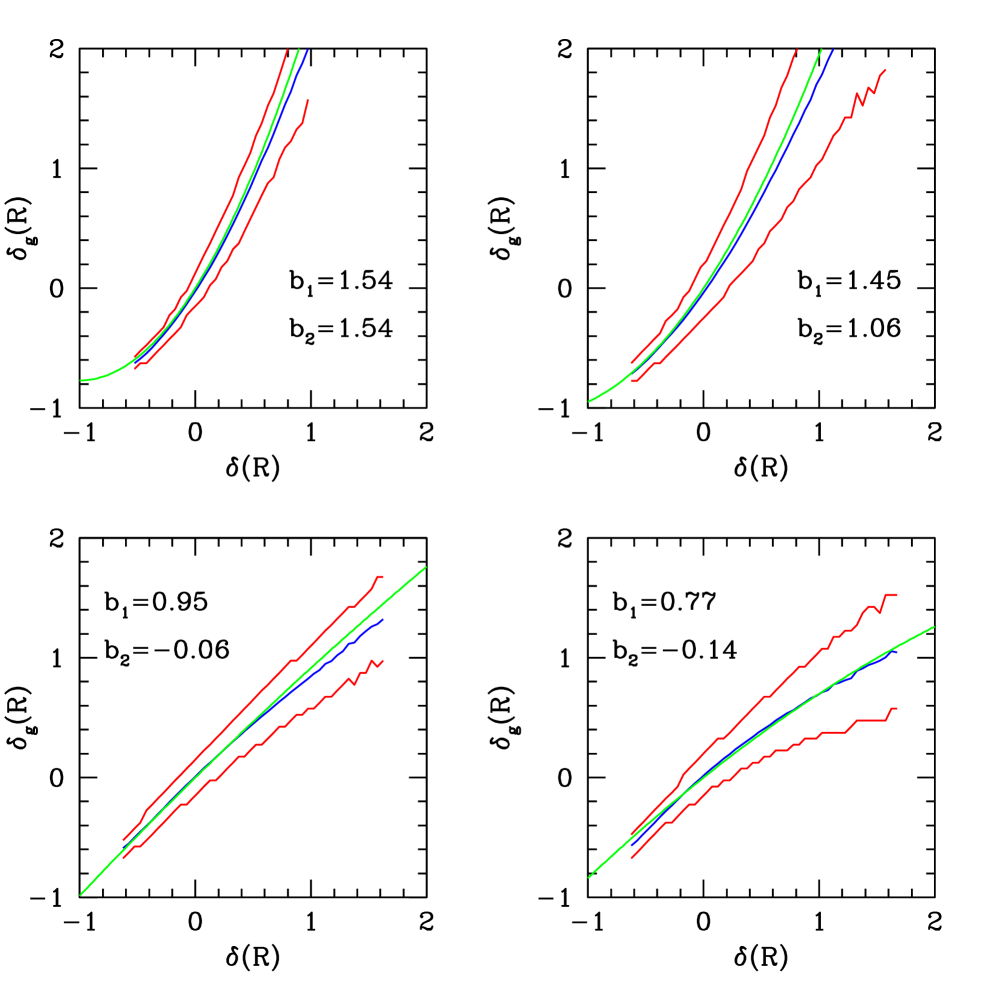
where $\nu({\mathchoice{{\hbox{\BFd x}}}{{\hbox{\BFt x}}}{{\hbox{\BFs x}}}{{\hbox{\BFss x}}}})\equiv\tilde{\delta}({\mathchoice{{\hbox{\BFd x}}}{{\hbox{\BFt x}}}{{\hbox{\BFs x}}}{{\hbox{\BFss x}}}})/\sigma$ is the local normalized smoothed density field. The model has two free parameters $a$ and $b$ that can be adjusted to generate stochastic biased fields that are preferentially weighted towards low or high density regions. The mass density field is generated using 2LPT (see description in Section 4.2 below) in a 300 Mpc/h box, with a $128^{3}$ grid. The smoothed density field in Eqs.(13-refproba) then corresponds to about 3 Mpc/h smoothing. For a given particle, we choose the nearest grid point to evaluate $\nu({\mathchoice{{\hbox{\BFd x}}}{{\hbox{\BFt x}}}{{\hbox{\BFs x}}}{{\hbox{\BFss x}}}})$, thus the biasing scheme is effectively non-local at scales of about 3 Mpc/h.

Figure 1 shows four examples of such a procedure. The top panels correspond to bias towards high density regions, with $b_{1}=b_{2}=1.54$ (left panel) and $b_{1}=1.45$, $b_{2}=1.06$ (right panel), whereas the bottom panels show examples of bias that preferentially select low density regions with $b_{1}=0.95$, $b_{2}=-0.06$ (left panel) and $b_{1}=0.77$, $b_{2}=-0.14$ (right panel). All except the bottom right panel are from $\Lambda$CDM realizations ($\Omega_{m}=0.3$, $\Omega_{\Lambda}=0.7$) with $\sigma_{8}=0.70$ for the dark matter. The bottom right panel corresponds to a $\tau$CDM realization ($\Omega_{m}=1$) with same normalization and power spectrum shape. The two right panels have roughly the same redshift distortions parameter $\beta\equiv\Omega_{m}^{0}.6/b_{1}\approx 0.65$, and thus will be nearly equal in terms of their redshift-space power spectrum. These bias parameter values in Figure 1 have been obtained by measuring the bispectrum for the “galaxy” distribution and comparing to the mass bispectrum using Eq. (3), and are plotted in each panel as the continuous solid line. The actual mean of the relation and its 90% confidence region for smoothed fields with Gaussian filter radius $R_{s}=10$Mpc/h show that even when the $\delta-\delta_{g}$ relation has considerable scatter, the bispectrum recovers the mean of the biasing relation quite accurately. Below, we shall discuss whether this result is also valid when dealing with noisy data such as in a galaxy survey, including the effects of survey geometry and sampling.

4 Numerical Implementation of PT: Comparison with N-body Simulations

4.1 The Need for Numerical PT

In order to understand how geometry and sampling affects statistics such as the bispectrum, we need to simulate galaxy catalogs and measure their statistical properties to compare with the ideal case known from analytical PT calculations and N-body simulations. As we shall see, it will be become very valuable to make a large number (a few hundred to a thousand) of mock catalogs for different cosmological models and survey selection functions. As a result, it would be very expensive to proceed with N-body simulations, even with PM simulations. Since we are interested in the large-scale properties of clustering, where PT applies, it is natural to resort to a numerical implementation of PT.

Lagrangian PT is the natural choice. In this formulation, particles are displaced from their initial positions by a displacement field that is found order by order perturbatively from the equations of motion. The linear solution is the well-known Zel’dovich (1970) approximation (ZA), and higher-order corrections have been well studied in the literature (Moutarde et al. (1991); Buchert et al. (1994); Bouchet et al. (1995)). Although the ZA is the least expensive of them, it does not reproduce very accurately the statistical properties of clustering even at large scales (Grinstein & Wise (1987); Juszkiewicz et al. (1993); Bernardeau 1994b ; Catelan & Moscardini (1994); Juszkiewicz et al. (1995)). In particular, we are interested in studying the bispectrum, and the ZA overestimates its configuration dependence and underestimates its overall amplitude. The situation becomes even worse as higher-order statistics are considered. To illustrate this, Table 1 shows the ratio of the $S_{p}$ parameters in the ZA to their exact values at large scales as a function of spectral index $n$. The $S_{p}$ parameters characterize the one-point PDF of the smoothed density field at scale $R$ (Goroff et al. (1986))

$$S_{p}\equiv\frac{\mathop{{}{\langle}{}}\tilde{\delta}^{p}\mathop{\rangle_{c}}}{\mathop{{}{\langle}{}}\tilde{\delta}^{2}\mathop{{}{\rangle}{}}^{p-1}},$$ (15)

and Table 1 shows $r_{p}\equiv S_{p}^{\rm ZA}/S_{p}$, where $S_{p}$ is the exact value calculated in full PT (Juszkiewicz et al. (1993); Bernardeau 1994a ; Bernardeau 1994b ). We see that for $p=3$ the skewness is poorly reproduced as the spectral index becomes positive, in the relevant range for CDM models at large scales. As a result, using the ZA to generate mock catalogs to study the statistical properties of the bispectrum could result in serious quantitative error.

The next level of accuracy is second-order Lagrangian PT (2LPT), which reproduces the three-point statistics (skewness and bispectrum) exactly, and gives reasonable values for higher-order statistics as well, in remarkable improvement over the ZA (Juszkiewicz et al. (1995)). Table 2 shows the analogous results for $r_{p}$ in 2LPT (Scoccimarro (1998)). Given the small additional computational expense of 2LPT over ZA (see discussion below), it is a very convenient scheme to implement for mock catalog production. It is still orders of magnitude faster than a PM simulation. The question then arises, is it worth to consider going beyond 2LPT? At third-order, 3LPT recovers four-point statistics exactly (see Table 3), but it involves an appreciable increase in complexity compared to 2LPT, requiring to solve three additional Poisson’s equations (Buchert et al. (1994)). For this reason, we consider 2LPT the optimal choice between speed and accuracy. We now briefly discuss 2LPT and its implementation.

4.2 Second-Order Lagrangian PT (2LPT)

In Lagrangian PT, the object of interest is the displacement field ${\bf\Psi}({\mathchoice{{\hbox{\BFd q}}}{{\hbox{\BFt q}}}{{\hbox{\BFs q}}}{{\hbox{\BFss q}}}})$ which maps the initial particle positions q into the final Eulerian particle positions x,

$${\mathchoice{{\hbox{\BFd x}}}{{\hbox{\BFt x}}}{{\hbox{\BFs x}}}{{\hbox{\BFss x}}}}={\mathchoice{{\hbox{\BFd q}}}{{\hbox{\BFt q}}}{{\hbox{\BFs q}}}{{\hbox{\BFss q}}}}+{\bf\Psi}({\mathchoice{{\hbox{\BFd q}}}{{\hbox{\BFt q}}}{{\hbox{\BFs q}}}{{\hbox{\BFss q}}}}).$$ (16)

The equation of motion for particle trajectories ${\mathchoice{{\hbox{\BFd x}}}{{\hbox{\BFt x}}}{{\hbox{\BFs x}}}{{\hbox{\BFss x}}}}(\tau)$ is

$$\frac{d^{2}{\mathchoice{{\hbox{\BFd x}}}{{\hbox{\BFt x}}}{{\hbox{\BFs x}}}{{\hbox{\BFss x}}}}}{d\tau^{2}}+{\cal H}(\tau)\ \frac{d{\mathchoice{{\hbox{\BFd x}}}{{\hbox{\BFt x}}}{{\hbox{\BFs x}}}{{\hbox{\BFss x}}}}}{d\tau}=-\nabla\Phi,$$ (17)

where $\Phi$ denotes the gravitational potential, and $\nabla$ the gradient operator in Eulerian coordinates x. Taking the divergence of this equation we obtain

$$J({\mathchoice{{\hbox{\BFd q}}}{{\hbox{\BFt q}}}{{\hbox{\BFs q}}}{{\hbox{\BFss q}}}},\tau)\ \nabla\cdot\Big{[}\frac{d^{2}{\mathchoice{{\hbox{\BFd x}}}{{\hbox{\BFt x}}}{{\hbox{\BFs x}}}{{\hbox{\BFss x}}}}}{d\tau^{2}}+{\cal H}(\tau)\ \frac{d{\mathchoice{{\hbox{\BFd x}}}{{\hbox{\BFt x}}}{{\hbox{\BFs x}}}{{\hbox{\BFss x}}}}}{d\tau}\Big{]}=\frac{3}{2}\Omega_{m}{\cal H}^{2}(J-1),$$ (18)

where we have used Poisson equation together with the fact that $1+\delta({\mathchoice{{\hbox{\BFd x}}}{{\hbox{\BFt x}}}{{\hbox{\BFs x}}}{{\hbox{\BFss x}}}})=J^{-1}$, and the Jacobian $J({\mathchoice{{\hbox{\BFd q}}}{{\hbox{\BFt q}}}{{\hbox{\BFs q}}}{{\hbox{\BFss q}}}},\tau)$ is the determinant

$$J({\mathchoice{{\hbox{\BFd q}}}{{\hbox{\BFt q}}}{{\hbox{\BFs q}}}{{\hbox{\BFss q}}}},\tau)\equiv{\rm Det}\Big{(}\delta_{ij}+\Psi_{i,j}\Big{)},$$ (19)

where $\Psi_{i,j}\equiv\partial\Psi_{i}/\partial{\mathchoice{{\hbox{\BFd q}}}{{\hbox{\BFt q}}}{{\hbox{\BFs q}}}{{\hbox{\BFss q}}}}_{j}$. Equation (18) can be fully rewritten in terms of Lagrangian coordinates by using that $\nabla_{i}=(\delta_{ij}+\Psi_{i,j})^{-1}\nabla_{q_{j}}$, where $\nabla_{q}\equiv\partial/\partial{\mathchoice{{\hbox{\BFd q}}}{{\hbox{\BFt q}}}{{\hbox{\BFs q}}}{{\hbox{\BFss q}}}}$ denotes the gradient operator in Lagrangian coordinates. The resulting non-linear equation for ${\bf\Psi}({\mathchoice{{\hbox{\BFd q}}}{{\hbox{\BFt q}}}{{\hbox{\BFs q}}}{{\hbox{\BFss q}}}})$ is then solved perturbatively, expanding about its linear solution, the Zel’dovich (1970) approximation

$$\nabla_{q}\cdot{\bf\Psi}^{(1)}=-D_{1}(\tau)\ \delta({\mathchoice{{\hbox{\BFd q}}}{{\hbox{\BFt q}}}{{\hbox{\BFs q}}}{{\hbox{\BFss q}}}}),$$ (20)

which incorporates the kinematic aspect of the collapse of fluid elements in Lagrangian space. Here $\delta({\mathchoice{{\hbox{\BFd q}}}{{\hbox{\BFt q}}}{{\hbox{\BFs q}}}{{\hbox{\BFss q}}}})$ denotes the (Gaussian) density field imposed by the initial conditions and $D_{1}(\tau)$ is the linear growth factor. The solution to second order describes the correction to the ZA displacement due to gravitational tidal effects and reads

$$\nabla_{q}\cdot{\bf\Psi}^{(2)}=\frac{1}{2}D_{2}(\tau)\sum_{i\neq j}(\Psi_{i,i}^{(1)}\Psi_{j,j}^{(1)}-\Psi_{i,j}^{(1)}\Psi_{j,i}^{(1)}),$$ (21)

(e.g., Bouchet et al. 1995) where $D_{2}(\tau)$ denotes the second-order growth factor, which for $0.1\leq\Omega_{m}\leq 3$ ($\Lambda=0$) obeys

$$D_{2}(\tau)\approx-\frac{3}{7}D_{1}^{2}(\tau)\ \Omega_{m}^{-2/63}\approx-\frac{3}{7}D_{1}^{2}(\tau)$$ (22)

to better than 0.5% and 7%, respectively (Bouchet et al. 1995), whereas for flat models with non-zero cosmological constant $\Lambda$ we have for $0.01\leq\Omega_{m}\leq 1$

$$D_{2}(\tau)\approx-\frac{3}{7}D_{1}^{2}(\tau)\ \Omega_{m}^{-1/143}\approx-\frac{3}{7}D_{1}^{2}(\tau),$$ (23)

to better than 0.6% and 2.6%, respectively (Bouchet et al. 1995). Since Lagrangian solutions up to second-order are curl-free, it is convenient to define Lagrangian potentials $\phi^{(1)}$ and $\phi^{(2)}$ so that in 2LPT

$${\mathchoice{{\hbox{\BFd x}}}{{\hbox{\BFt x}}}{{\hbox{\BFs x}}}{{\hbox{\BFss x}}}}({\mathchoice{{\hbox{\BFd q}}}{{\hbox{\BFt q}}}{{\hbox{\BFs q}}}{{\hbox{\BFss q}}}})={\mathchoice{{\hbox{\BFd q}}}{{\hbox{\BFt q}}}{{\hbox{\BFs q}}}{{\hbox{\BFss q}}}}-D_{1}\ \nabla_{q}\phi^{(1)}+D_{2}\ \nabla_{q}\phi^{(2)},$$ (24)

and the velocity field then reads ($t$ denotes cosmic time)

$${\bf v}\equiv\frac{d{\mathchoice{{\hbox{\BFd x}}}{{\hbox{\BFt x}}}{{\hbox{\BFs x}}}{{\hbox{\BFss x}}}}}{dt}=-D_{1}\ f_{1}\ H\ \nabla_{q}\phi^{(1)}+D_{2}\ f_{2}\ H\ \nabla_{q}\phi^{(2)},$$ (25)

where $H$ is the Hubble constant, and the logarithmic derivatives of the growth factors $f_{i}\equiv(d\ln D_{i})/(d\ln a)$ can be approximated for open models with $0.1\leq\Omega_{m}\leq 1$ by

$$f_{1}\approx\Omega_{m}^{3/5},\ \ \ \ \ f_{2}\approx 2\ \Omega_{m}^{4/7},$$ (26)

to better than 2% (Peebles 1976) and 5% (Bouchet et al. 1995), respectively. For flat models with non-zero cosmological constant $\Lambda$ we have for $0.01\leq\Omega_{m}\leq 1$

$$f_{1}\approx\Omega_{m}^{5/9},\ \ \ \ \ f_{2}\approx 2\ \Omega_{m}^{6/11},$$ (27)

to better than 10% and 12%, respectively (Bouchet et al. 1995). The accuracy of these two fits improves significantly for $\Omega_{m}\geq 0.1$, in the range relevant for the present purposes. The time-independent potentials in Eqs. (24) and (25) obey the following Poisson equations (Buchert et al. 1994)

$$\nabla_{q}^{2}\phi^{(1)}({\mathchoice{{\hbox{\BFd q}}}{{\hbox{\BFt q}}}{{\hbox{\BFs q}}}{{\hbox{\BFss q}}}}) = \delta({\mathchoice{{\hbox{\BFd q}}}{{\hbox{\BFt q}}}{{\hbox{\BFs q}}}{{\hbox{\BFss q}}}}),$$ (28)

$$\nabla_{q}^{2}\phi^{(2)}({\mathchoice{{\hbox{\BFd q}}}{{\hbox{\BFt q}}}{{\hbox{\BFs q}}}{{\hbox{\BFss q}}}}) = \sum_{i>j}[\phi_{,ii}^{(1)}({\mathchoice{{\hbox{\BFd q}}}{{\hbox{\BFt q}}}{{\hbox{\BFs q}}}{{\hbox{\BFss q}}}})\ \phi_{,jj}^{(1)}({\mathchoice{{\hbox{\BFd q}}}{{\hbox{\BFt q}}}{{\hbox{\BFs q}}}{{\hbox{\BFss q}}}})-(\phi_{,ij}^{(1)}({\mathchoice{{\hbox{\BFd q}}}{{\hbox{\BFt q}}}{{\hbox{\BFs q}}}{{\hbox{\BFss q}}}}))^{2}],$$ (29)

4.3 Regime of Validity

In order to assess the validity of 2LPT, we have run N-body simulations using the Hydra adaptive P³M code (Couchman, Thomas & Pearce (1995)). We have run 4 realizations of $\Lambda$CDM ($\Omega_{m}=0.3$, $\Omega_{\Lambda}=0.7$, $\sigma_{8}=0.90$) and 2 realizations of SCDM ($\sigma_{8}=0.61$), using a 300 Mpc/h box, with $128^{3}$ particles and softening length $\epsilon=0.25$ Mpc/h. The 2LPT realizations were made using in most cases $256^{3}$ particles in a 600 Mpc/h box (identical results are obtained using 300 Mpc/h boxes).

We now use the results of these simulations to check the regime of validity of 2LPT. We shall concentrate on power spectrum and bispectrum statistics, in real and redshift space. When dealing with Lagrangian PT, a signature of its breakdown is the amount of shell crossing; the fact that the Jacobian in Eq. (19) becomes zero at the regions where particles (initially at different positions) cross each other. This effect is well-known in the ZA, and leads to the “thickening of pancakes”, that is, to significant smoothing of high density regions. A way of characterizing this effect is to recall that the density field in the ZA is given by

$$1+\delta({\mathchoice{{\hbox{\BFd x}}}{{\hbox{\BFt x}}}{{\hbox{\BFs x}}}{{\hbox{\BFss x}}}})=\frac{1}{J({\mathchoice{{\hbox{\BFd q}}}{{\hbox{\BFt q}}}{{\hbox{\BFs q}}}{{\hbox{\BFss q}}}},\tau)}=\frac{1}{\prod_{i=1}^{3}(1+\lambda_{i}({\mathchoice{{\hbox{\BFd q}}}{{\hbox{\BFt q}}}{{\hbox{\BFs q}}}{{\hbox{\BFss q}}}},\tau))},$$ (30)

where $\lambda_{i}$ denotes the eigenvalues of the first-order deformation tensor $\Psi_{i,j}^{(1)}$ at point q and time $\tau$ [see Eq. 19]. The condition for shell-crossing can then be explicitly written as $1+\lambda_{i}({\mathchoice{{\hbox{\BFd q}}}{{\hbox{\BFt q}}}{{\hbox{\BFs q}}}{{\hbox{\BFss q}}}},\tau)=0$, for any $i=1,2,3$. At these points, one expects not only a breakdown of the ZA, but also of higher-order Lagrangian PT, in particular 2LPT. An alternative indicator of the breakdown of 2LPT, as in any perturbative approach, is to compare the magnitude of the second-order to the first-order displacement field. One expects 2LPT will break down when the second-order contribution becomes significant compared to the ZA.

Table 4 shows these indicators in 2LPT realizations as described above for $\Lambda$CDM with normalization $\sigma_{8}=0.7$. In order to investigate the dependence of the breakdown of 2LPT with the amount of small-scale power, we include a cutoff in the linear power spectrum so that $P_{lin}(k)=0$ for $k>k_{c}$. As more high-frequency waves are included in the representation of the linear density field, one expects 2LPT to break down at larger scales. On the other hand, not enough waves lead to lack of mode-coupling, and therefore inaccurate representation of the density field one is trying to simulate. Thus there is an “optimum” cutoff; here we considered models with $k_{c}=0.3,0.4,0.5,\infty$ h/Mpc.

In Table 4 we show much shell crossing is developed as a function of $k_{c}$, in terms of the quantity $x_{sc}\equiv 100\times N_{sc}/N_{grid}^{3}$, where $N_{sc}$ is the number of grid points that obeyed the shell-crossing condition ($|\lambda_{i}|\geq 1$ for at least one $i=1,2,3$), and $N_{grid}$ is the total number of grid points (where particles are initially located, $N_{par}=N_{grid}^{3}$). Obviously, $x_{sc}$ is an increasing function of $k_{c}$. The remaining column in Table 4 shows the ratio of mean second to first-order displacement field magnitudes. Again, this ratio increases with $k_{c}$, as expected. We see that even though this ratio is always less than unity, significant shell crossing develops (e.g. for $k_{c}>0.5$), so breakdown of 2LPT is nonetheless expected to happen. In the following we use 2LPT realizations with $k_{c}=0.5$ h/Mpc, which we found reproduces clustering statistics in redshift space very well.

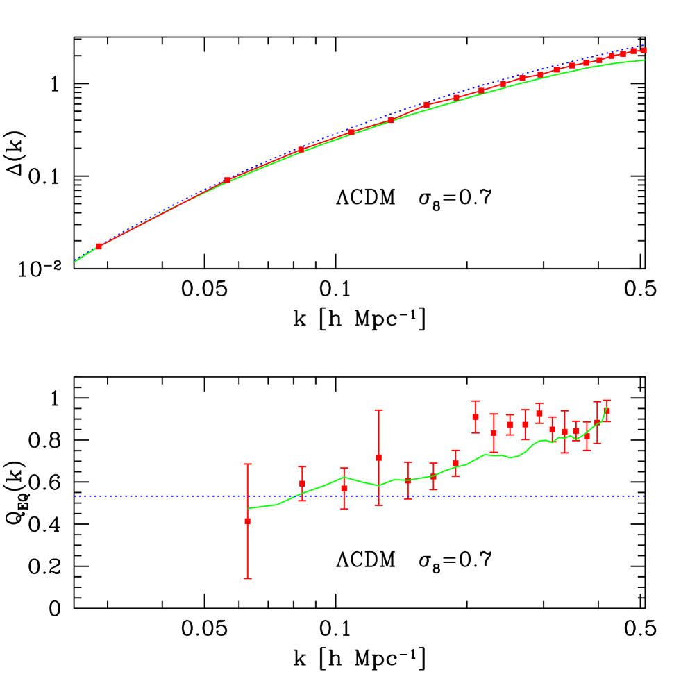
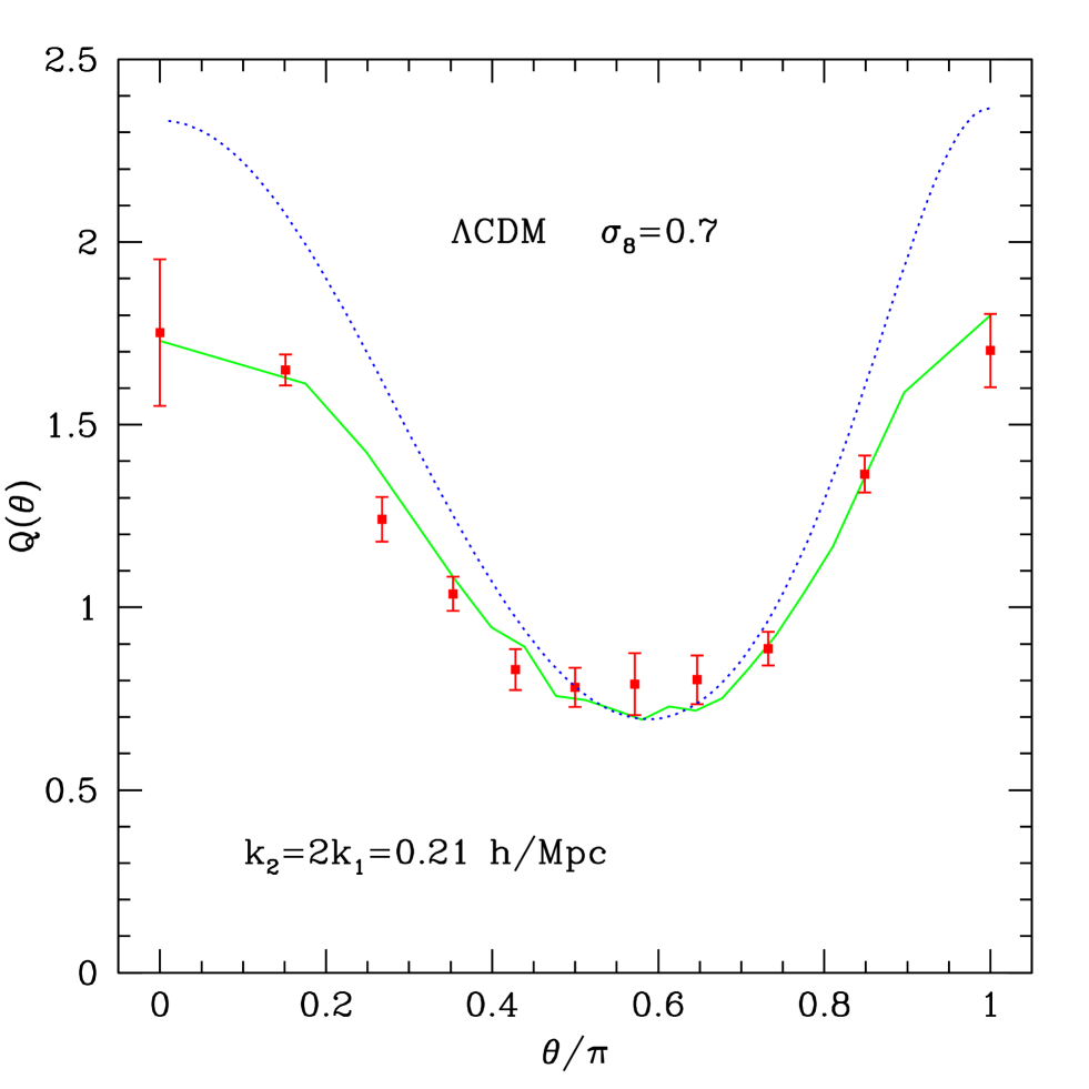
In Figure 2 we show a comparison of 2LPT (solid lines) with N-body simulations (symbols) in redshift space. The top panel shows the power spectrum (in terms of $\Delta(k)=4\pi k^{3}P(k)$) as a function of scale, the dotted line corresponds to linear PT, Eq. 33 below (Kaiser 1987). At large scales, $k<0.2$ h/Mpc, 2LPT reproduces the suppresion of power compared to linear PT; at smaller scales the supression is overestimated, as we approach the cutoff scale of the power spectrum and also shell crossing starts playing a role. The bottom panel shows a similar comparison for the equilateral bispectrum, the dotted line now corresponds to the redshift space prediction at large scales from tree-level PT (Scoccimarro et al. 1999). We see that although tree-level PT breaks down at about $k\approx 0.2$ h/Mpc, 2LPT continues to hold at smaller scales, $k\leq 0.4$ h/Mpc. Figure 3 shows a comparison for the redshift space bispectrum for configurations in which $k_{2}=2k_{1}=0.21$ h/Mpc as a function of the angle $\theta$ between ${\mathchoice{{\hbox{\BFd k}}}{{\hbox{\BFt k}}}{{\hbox{\BFs k}}}{{\hbox{\BFss k}}}}_{1}$ and ${\mathchoice{{\hbox{\BFd k}}}{{\hbox{\BFt k}}}{{\hbox{\BFs k}}}{{\hbox{\BFss k}}}}_{2}$. The dotted line shows the prediction of tree-level PT (Hivon et al. 1995). As noted before (Scoccimarro et al 1999), the predictions of tree-level PT in redshift space break down at relatively large scales, due to the non-perturbative nature of the redshift-space mapping. Fortunately, since 2LPT performs the mapping exactly, the agreement with the numerical simulations is very good down to scales $k\approx 0.4$ h/Mpc. For our purposes, we are interested in studying statistics at large scales, $k\leq 0.2$ h/Mpc (with $k_{nl}>0.2$ h/Mpc), so the use of 2LPT is well justified.

5 Redshift Distortions

5.1 Plane-Parallel Approximation

In redshift space, the radial coordinate s of a galaxy is given by its observed radial velocity, a combination of its Hubble flow plus “distortions” due to peculiar velocities. The mapping from real-space position x to redshift space is given by:

$${\mathchoice{{\hbox{\BFd s}}}{{\hbox{\BFt s}}}{{\hbox{\BFs s}}}{{\hbox{\BFss s}}}}={\mathchoice{{\hbox{\BFd x}}}{{\hbox{\BFt x}}}{{\hbox{\BFs x}}}{{\hbox{\BFss x}}}}-f\ {\hbox{$u_{z}$}}({\mathchoice{{\hbox{\BFd x}}}{{\hbox{\BFt x}}}{{\hbox{\BFs x}}}{{\hbox{\BFss x}}}}){\hat{z}},$$ (31)

where $f(\Omega_{m})\approx\Omega_{m}^{0.6}$ is the logarithmic growth rate of linear perturbations, and ${\mathchoice{{\hbox{\BFd u}}}{{\hbox{\BFt u}}}{{\hbox{\BFs u}}}{{\hbox{\BFss u}}}}({\mathchoice{{\hbox{\BFd x}}}{{\hbox{\BFt x}}}{{\hbox{\BFs x}}}{{\hbox{\BFss x}}}})\equiv-{\mathchoice{{\hbox{\BFd v}}}{{\hbox{\BFt v}}}{{\hbox{\BFs v}}}{{\hbox{\BFss v}}}}({\mathchoice{{\hbox{\BFd x}}}{{\hbox{\BFt x}}}{{\hbox{\BFs x}}}{{\hbox{\BFss x}}}})/({\cal H}f)$, where ${\mathchoice{{\hbox{\BFd v}}}{{\hbox{\BFt v}}}{{\hbox{\BFs v}}}{{\hbox{\BFss v}}}}({\mathchoice{{\hbox{\BFd x}}}{{\hbox{\BFt x}}}{{\hbox{\BFs x}}}{{\hbox{\BFss x}}}})$ is the peculiar velocity field, and ${\cal H}(\tau)\equiv(1/a)(da/d\tau)=Ha$ is the conformal Hubble parameter (with FRW scale factor $a(\tau)$ and conformal time $\tau$). In Eq. (31), we have assumed the “plane-parallel” approximation, so that the line-of-sight is taken as a fixed direction, denoted by ${\hat{z}}$. Using this mapping, the Fourier transform of the density field contrast in redshift space reads (Scoccimarro et al. (1999))

$$\delta_{s}({\mathchoice{{\hbox{\BFd k}}}{{\hbox{\BFt k}}}{{\hbox{\BFs k}}}{{\hbox{\BFss k}}}})=\int\frac{d^{3}x}{(2\pi)^{3}}{\rm e}^{-i{\mathchoice{{\hbox{\BFd k}}}{{\hbox{\BFt k}}}{{\hbox{\BFs k}}}{{\hbox{\BFss k}}}}\cdot{\mathchoice{{\hbox{\BFd x}}}{{\hbox{\BFt x}}}{{\hbox{\BFs x}}}{{\hbox{\BFss x}}}}}{\rm e}^{ifk_{z}{\hbox{$u_{z}$}}({\mathchoice{{\hbox{\BFd x}}}{{\hbox{\BFt x}}}{{\hbox{\BFs x}}}{{\hbox{\BFss x}}}})}\Big{[}\delta({\mathchoice{{\hbox{\BFd x}}}{{\hbox{\BFt x}}}{{\hbox{\BFs x}}}{{\hbox{\BFss x}}}})+f\nabla_{z}{\hbox{$u_{z}$}}({\mathchoice{{\hbox{\BFd x}}}{{\hbox{\BFt x}}}{{\hbox{\BFs x}}}{{\hbox{\BFss x}}}})\Big{]}.$$ (32)

This equation describes the fully non-linear density field in redshift space in the plane-parallel approximation. In linear perturbation theory, the exponential factor becomes unity, and we recover the well known formula (Kaiser (1987))

$$\delta_{s}({\mathchoice{{\hbox{\BFd k}}}{{\hbox{\BFt k}}}{{\hbox{\BFs k}}}{{\hbox{\BFss k}}}})=\delta({\mathchoice{{\hbox{\BFd k}}}{{\hbox{\BFt k}}}{{\hbox{\BFs k}}}{{\hbox{\BFss k}}}})\ (1+f\mu^{2}).$$ (33)

Given the general formula, Eq. (32), and the local biasing scheme in Eq. (2) (with $\varepsilon({\mathchoice{{\hbox{\BFd x}}}{{\hbox{\BFt x}}}{{\hbox{\BFs x}}}{{\hbox{\BFss x}}}})=0$), it is easy to work out the perturbative solutions order by order (Scoccimarro et al. (1999)). Let’s write the Fourier components of the density field in redshift space as

$$\delta_{s}({\mathchoice{{\hbox{\BFd k}}}{{\hbox{\BFt k}}}{{\hbox{\BFs k}}}{{\hbox{\BFss k}}}}) = \sum_{n=1}^{\infty}D_{1}^{n}\int[\delta_{\rm D}]_{n}\ Z_{n}({\mathchoice{{\hbox{\BFd k}}}{{\hbox{\BFt k}}}{{\hbox{\BFs k}}}{{\hbox{\BFss k}}}}_{1},\ldots,{\mathchoice{{\hbox{\BFd k}}}{{\hbox{\BFt k}}}{{\hbox{\BFs k}}}{{\hbox{\BFss k}}}}_{n})\ \prod_{i=1}^{n}\delta_{1}({\mathchoice{{\hbox{\BFd k}}}{{\hbox{\BFt k}}}{{\hbox{\BFs k}}}{{\hbox{\BFss k}}}}_{i})\ d^{3}k_{i},$$

where $Z_{n}$ are dimensionless, symmetric, scalar functions of their arguments, $D_{1}$ is the linear growth factor of the density field, and $[\delta_{\rm D}]_{n}\equiv\delta_{D}({\mathchoice{{\hbox{\BFd k}}}{{\hbox{\BFt k}}}{{\hbox{\BFs k}}}{{\hbox{\BFss k}}}}-{\mathchoice{{\hbox{\BFd k}}}{{\hbox{\BFt k}}}{{\hbox{\BFs k}}}{{\hbox{\BFss k}}}}_{1}\ldots-{\mathchoice{{\hbox{\BFd k}}}{{\hbox{\BFt k}}}{{\hbox{\BFs k}}}{{\hbox{\BFss k}}}}_{n})$. In particular the first and second-order PT kernels are (Hivon et al. (1995); Verde et al. (1998); Scoccimarro et al. (1999))

$$Z_{1}({\mathchoice{{\hbox{\BFd k}}}{{\hbox{\BFt k}}}{{\hbox{\BFs k}}}{{\hbox{\BFss k}}}}) = (b_{1}+f\mu^{2})$$ (35)

$$Z_{2}({\mathchoice{{\hbox{\BFd k}}}{{\hbox{\BFt k}}}{{\hbox{\BFs k}}}{{\hbox{\BFss k}}}}_{1},{\mathchoice{{\hbox{\BFd k}}}{{\hbox{\BFt k}}}{{\hbox{\BFs k}}}{{\hbox{\BFss k}}}}_{2}) = \frac{b_{2}}{2}+b_{1}F_{2}({\mathchoice{{\hbox{\BFd k}}}{{\hbox{\BFt k}}}{{\hbox{\BFs k}}}{{\hbox{\BFss k}}}}_{1},{\mathchoice{{\hbox{\BFd k}}}{{\hbox{\BFt k}}}{{\hbox{\BFs k}}}{{\hbox{\BFss k}}}}_{2})+f\mu^{2}G_{2}({\mathchoice{{\hbox{\BFd k}}}{{\hbox{\BFt k}}}{{\hbox{\BFs k}}}{{\hbox{\BFss k}}}}_{1},{\mathchoice{{\hbox{\BFd k}}}{{\hbox{\BFt k}}}{{\hbox{\BFs k}}}{{\hbox{\BFss k}}}}_{2})+\frac{f\mu k}{2}\Big{[}\frac{\mu_{1}}{k_{1}}(b_{1}+f\mu_{2}^{2})+\frac{\mu_{2}}{k_{2}}(b_{1}+f\mu_{1}^{2})\Big{]},$$ (36)

where we denote $\mu\equiv{\mathchoice{{\hbox{\BFd k}}}{{\hbox{\BFt k}}}{{\hbox{\BFs k}}}{{\hbox{\BFss k}}}}\cdot{\hat{z}}/k$, with ${\mathchoice{{\hbox{\BFd k}}}{{\hbox{\BFt k}}}{{\hbox{\BFs k}}}{{\hbox{\BFss k}}}}\equiv{\mathchoice{{\hbox{\BFd k}}}{{\hbox{\BFt k}}}{{\hbox{\BFs k}}}{{\hbox{\BFss k}}}}_{1}+\ldots+{\mathchoice{{\hbox{\BFd k}}}{{\hbox{\BFt k}}}{{\hbox{\BFs k}}}{{\hbox{\BFss k}}}}_{n}$, and $\mu_{i}\equiv{\mathchoice{{\hbox{\BFd k}}}{{\hbox{\BFt k}}}{{\hbox{\BFs k}}}{{\hbox{\BFss k}}}}_{i}\cdot{\hat{z}}/k_{i}$. As in Eq. (7), $G_{2}$ denotes the second-order kernels for the velocity-divergence field, given by Eq. (8) after replacing $5/7\rightarrow 3/7$ and $2/7\rightarrow 4/7$. We can now write the power spectrum and bispectrum in redshift-space,

$$P_{s}({\mathchoice{{\hbox{\BFd k}}}{{\hbox{\BFt k}}}{{\hbox{\BFs k}}}{{\hbox{\BFss k}}}})=Z_{1}({\mathchoice{{\hbox{\BFd k}}}{{\hbox{\BFt k}}}{{\hbox{\BFs k}}}{{\hbox{\BFss k}}}})^{2}\ P(k),$$ (37)

$$B_{123}=2Z_{2}({\mathchoice{{\hbox{\BFd k}}}{{\hbox{\BFt k}}}{{\hbox{\BFs k}}}{{\hbox{\BFss k}}}}_{1},{\mathchoice{{\hbox{\BFd k}}}{{\hbox{\BFt k}}}{{\hbox{\BFs k}}}{{\hbox{\BFss k}}}}_{2})Z_{1}({\mathchoice{{\hbox{\BFd k}}}{{\hbox{\BFt k}}}{{\hbox{\BFs k}}}{{\hbox{\BFss k}}}}_{1})Z_{1}({\mathchoice{{\hbox{\BFd k}}}{{\hbox{\BFt k}}}{{\hbox{\BFs k}}}{{\hbox{\BFss k}}}}_{2})\ P(k_{1})P(k_{2})+{\rm cyc.}$$ (38)

Note that both statistics do now depend on the direction of the wave vectors with respect to the line of sight, since the redshift-space mapping in the plane-parallel approximation breaks statistical isotropy. One can proceed to decompose these statistics in multipole moments; however, in this paper we will be dealing exclusively with their monopoles. The resulting reduced bispectrum $Q$, defined as in Eq. (1) in terms of monopole quantities, now becomes a function of $\beta\equiv f/b_{1}$, $b_{1}$ and $b_{2}$. Even though Eq. (3) is not valid anymore in redshift-space, it is still a reasonable approximation (Scoccimarro et al. (1999)). As a result, even including redshift-distortions, the reduced bispectrum $Q$ is weakly sensitive to $\Omega_{m}$ (or $\beta$) (Hivon et al. (1995); Verde et al. (1998); Scoccimarro et al. (1999)).

5.2 Effect of Radial Redshift-Distortions

A standard procedure with redshift distortions is to treat them in the plane-parallel approximation (Kaiser (1987)). When dealing with surveys with substantial sky coverage, this approximation is expected to break down. In an all-sky survey (as IRAS ) the radial character of redshift distortions mean that clustering statistics are statistically isotropic but inhomogeneous (rather than statistically homogeneous but anisotropic, as in the plane-parallel case). The breakdown of statistical homogeneity means that Fourier modes are not independent anymore, in particular, the power spectrum is not diagonal, e.g. different band powers are correlated, even in the linear regime (Zaroubi & Hoffman (1996)).

We will show, however, that for the monopole of the power spectrum and bispectrum in the all-sky case, radial and plane-parallel distortions agree with each other extremely well. This can be understood from the fact that the monopole is not sensitive to the orientation of structures but to the overall spherical average of power. On the other hand, higher-order multipoles (and thus the full unaveraged over angles statistics) such as the quadrupole are much more sensitive to the radial character of the distortions; in fact, in the limit of full sky, the anisotropy (with respect to a fixed direction) vanishes.

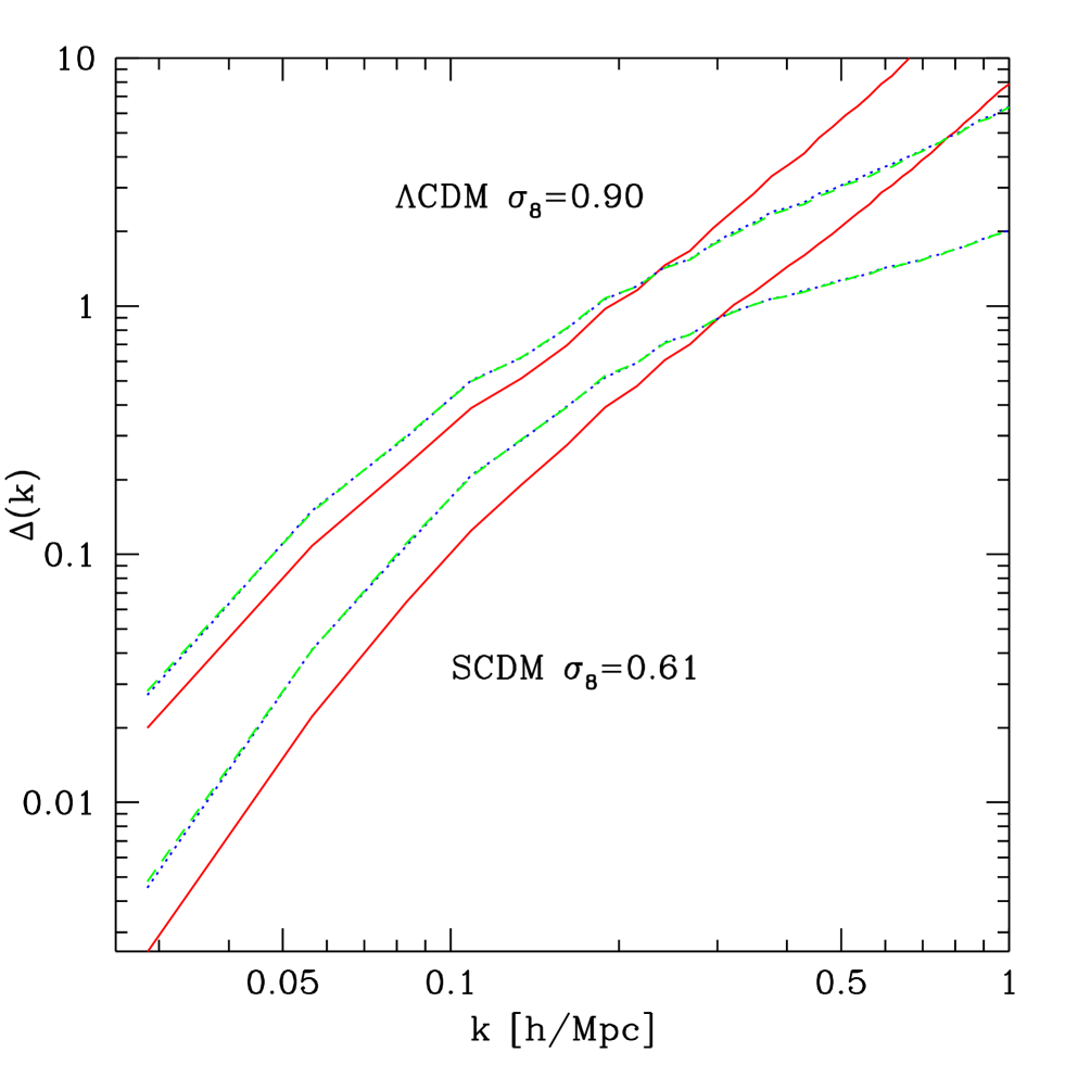
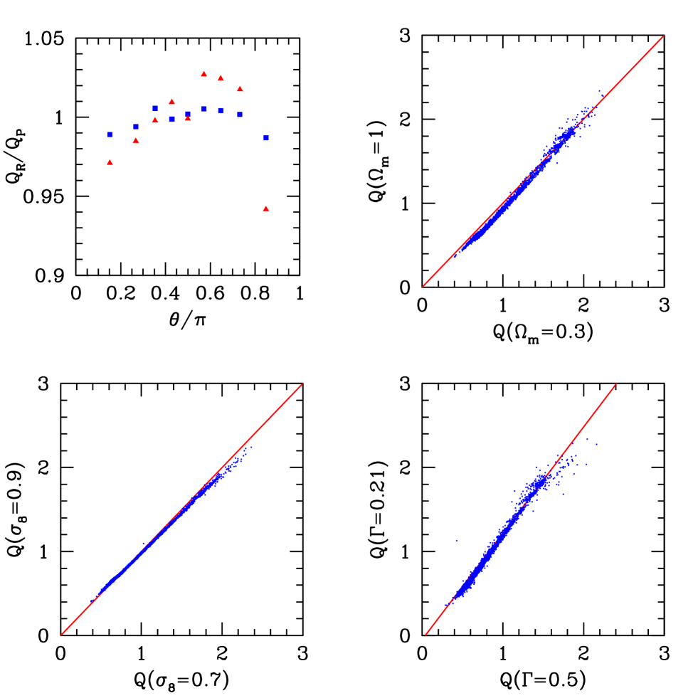
Figure 4 illustrates this for the monopole of the power spectrum. Solid lines denote the undistorted non-linear power spectrum, whereas dotted (dashed) lines denote the power spectrum monopole under radial (plane-parallel) redshift-space mapping. The radial results overlap with the plane-parallel ones except for a very small difference at large scales, where the radial results are slightly smaller. This is indeed expected at the 10% level for the scales plotted (Heavens & Taylor (1995)). A similar result holds for the scale dependence of the bispectrum. In the top left panel of Fig. 5 we show the ratio of the bispectrum under radial ($Q_{R}$) to plane-parallel ($Q_{P}$) redshift-space mapping as a function of the angle $\theta$ between ${\mathchoice{{\hbox{\BFd k}}}{{\hbox{\BFt k}}}{{\hbox{\BFs k}}}{{\hbox{\BFss k}}}}_{1}$ and ${\mathchoice{{\hbox{\BFd k}}}{{\hbox{\BFt k}}}{{\hbox{\BFs k}}}{{\hbox{\BFss k}}}}_{2}$ for $k_{2}=2k_{1}=0.105$ h/Mpc (triangles) and $k_{2}=2k_{1}=0.21$ h/Mpc (squares). In order to get this result we have averaged over 200 realizations of $\Lambda$CDM. There is an apparent trend at the few percent level that indicates that under the radial mapping the configuration dependence is very slightly suppressed, but the effect is very small even at these large scales. In the following we use radial distortions, although for our purposes plane-parallel approximation would have been a good approximation. We use Fourier modes even though they are not the natural set of modes anymore in the presence of radial redshift-distortions (see e.g. Heavens & Taylor (1995); Hamilton & Culhane 1996).

5.3 Dependence of $Q$ on Cosmology and Power Spectrum

As discussed before, $Q$ depends mainly on the spectral index, biasing, Gaussianity of initial conditions, and it is quite insensitive to the matter density $\Omega_{m}$ and should be independent to leading order on the power spectrum normalization $\sigma_{8}$. We now quantify these dependences in the presence of non-linear redshift distortions. Figure 5 shows the results of averaging 200 realizations of 2LPT, as described before, for different models. The top right panel shows the dependence of $Q$ on the matter density parameter $\Omega_{m}$, for power spectrum shape given by $\Gamma=0.21$. The scatter plot corresponds to measurements of $Q$ in all triangles (4741 in total) between scales of $k=0.05$ h/Mpc and $k=0.2$ h/Mpc. Equilateral triangles correspond to the small amplitude region (lower left corner), whereas colinear triangles ocupy the upper right corner. As predicted by tree-level PT, the $\Omega_{m}=1$ case shows a higher colinear amplitude and lower equilateral amplitude than the $\Omega_{m}=0.3$ case, although the precise value of these amplitudes does not quite agree with tree-level PT in the presence of non-linear redshift distortions, as we saw in Fig. 3. The effect of a change in $\Omega_{m}$ is of the order of $10\%$ (Hivon et al. 1995).

The bottom left panel shows the effect of changing $\sigma_{8}$ for $\Lambda$CDM models. As we see, non-linear redshift distortions introduce a very small dependence, with larger $\sigma_{8}$ leading to a slightly smaller configuration dependence of $Q$, but the effect is negligible for the analysis of IRAS surveys given the error bars involved, as we shall see. On the other hand, as expected, the dependence on the shape of the power spectrum, parameterized by $\Gamma$ in CDM models is quite strong due to a change of the spectral index with scale. We see from the bottom right panel that for $\Omega_{m}=1$, a $\Gamma=0.5$ has a much weaker configuration dependence than a $\Omega_{m}=0.21$, as expected since the spectral index of the latter is more negative at a given scale. The solid line in this panel shows the relation $Q(\Gamma=0.21)=1.3Q(\Gamma=0.5)-0.05$, which fits the results quite well. As a result of this, a $\Gamma=0.5$ model when compared with a given galaxy bispectrum will lead to smaller values for the bias parameters $b_{1}$ and $b_{2}$ than a $\Gamma=0.21$ model, assuming no other constraint is imposed.

6 Mock Catalogs: Selection Functions and Optimal Weighing

We generate mock catalogs of different surveys by the following procedure. We use 2LPT to generate density and velocity fields for a given cosmological model and normalization $\sigma_{8}$. In most cases we use $128^{3}$ particles in a 600 Mpc/h box, for biased galaxy distributions we use a parent $200^{3}$ 2LPT realization from which an $\approx 128^{3}$ distribution is generated (see below). An observer is then picked at random with velocity consistent with that of the local group with respect to the CMB frame. The full (radial) redshift-space mapping is performed using the velocity field, to obtain the redshift-space distribution. Given the particle distribution in redshift-space, “galaxies” are selected using the desired IRAS survey selection function, replicating the box if necessary, including the galactic cut, and rejecting galaxies closer than 20 Mpc/h from the observer. The selection functions are given by:

$$n(r)=\frac{A}{r^{2}}\frac{\left(r/r_{0}\right)^{a}}{1+\left(r/r_{0}\right)^{b}},$$ (39)

with parameters given in Table 5. These were kindly provided by H. Feldman, and obtained by fitting the actual redshift distribution observed in the different IRAS surveys.

In order to correct for the selection function and the geometry of the survey, we use the standard FKP method (Feldman et al. (1994); hereafter FKP). For each realization of the mock survey, a corresponding random catalogue is generated using the same geometry and selection function, but about ten times more dense. We then measure statistics (power spectrum and bispectrum monopoles) for the auxiliary $F({\mathchoice{{\hbox{\BFd k}}}{{\hbox{\BFt k}}}{{\hbox{\BFs k}}}{{\hbox{\BFss k}}}})$ field,

$$F({\mathchoice{{\hbox{\BFd k}}}{{\hbox{\BFt k}}}{{\hbox{\BFs k}}}{{\hbox{\BFss k}}}})=\int d^{3}x\ w_{k}({\mathchoice{{\hbox{\BFd x}}}{{\hbox{\BFt x}}}{{\hbox{\BFs x}}}{{\hbox{\BFss x}}}})\left[n_{g}({\mathchoice{{\hbox{\BFd x}}}{{\hbox{\BFt x}}}{{\hbox{\BFs x}}}{{\hbox{\BFss x}}}})-\alpha n_{r}({\mathchoice{{\hbox{\BFd x}}}{{\hbox{\BFt x}}}{{\hbox{\BFs x}}}{{\hbox{\BFss x}}}})\right]\exp(i{\mathchoice{{\hbox{\BFd k}}}{{\hbox{\BFt k}}}{{\hbox{\BFs k}}}{{\hbox{\BFss k}}}}\cdot{\mathchoice{{\hbox{\BFd x}}}{{\hbox{\BFt x}}}{{\hbox{\BFs x}}}{{\hbox{\BFss x}}}}),$$ (40)

where $n_{g}({\mathchoice{{\hbox{\BFd x}}}{{\hbox{\BFt x}}}{{\hbox{\BFs x}}}{{\hbox{\BFss x}}}})$ and $n_{r}({\mathchoice{{\hbox{\BFd x}}}{{\hbox{\BFt x}}}{{\hbox{\BFs x}}}{{\hbox{\BFss x}}}})$ are the galaxy and random catalog density fields, and $\alpha=N_{g}/N_{r}$ scales the overall random density to the survey density. Note that the use of a random catalog is not necessary, one could just as well use the survey selection function multiplied by the survey mask to substract the expected shot noise; or even better, substract the “actual” shot noise using the data itself (Hamilton 1997). The weight function $w_{k}({\mathchoice{{\hbox{\BFd x}}}{{\hbox{\BFt x}}}{{\hbox{\BFs x}}}{{\hbox{\BFss x}}}})\equiv 1/\left[1+\bar{n}P(k)\right]$ is chosen as to minimize the variance of the power spectrum estimator at scales small compared to the survey size (FKP). In fact, under the same assumptions plus Gaussian errors, the same weight function minimizes the variance of the higher-order correlation functions as well. Indeed, the variance $(\Delta\hat{T}_{m})^{2}$ in the estimator of the $m-$point spectrum $\hat{T}_{m}$ in this limit is

$$(\Delta\hat{T}_{m})^{2}\sim\frac{\int d^{3}x\ n^{2m}({\mathchoice{{\hbox{\BFd x}}}{{\hbox{\BFt x}}}{{\hbox{\BFs x}}}{{\hbox{\BFss x}}}})\prod_{i=1}^{m}\left[P(k_{i})+1/n\right]w_{k_{i}}^{2}({\mathchoice{{\hbox{\BFd x}}}{{\hbox{\BFt x}}}{{\hbox{\BFs x}}}{{\hbox{\BFss x}}}})}{\left[\int d^{3}x\ n^{m}({\mathchoice{{\hbox{\BFd x}}}{{\hbox{\BFt x}}}{{\hbox{\BFs x}}}{{\hbox{\BFss x}}}})\prod_{i=1}^{m}w_{k_{i}}^{2}({\mathchoice{{\hbox{\BFd x}}}{{\hbox{\BFt x}}}{{\hbox{\BFs x}}}{{\hbox{\BFss x}}}})\right]^{2}},$$ (41)

and taking variations with respect to the weight function $w_{k_{j}}({\mathchoice{{\hbox{\BFd r}}}{{\hbox{\BFt r}}}{{\hbox{\BFs r}}}{{\hbox{\BFss r}}}})$ it follows that

$$\frac{w_{k_{j}}({\mathchoice{{\hbox{\BFd r}}}{{\hbox{\BFt r}}}{{\hbox{\BFs r}}}{{\hbox{\BFss r}}}})[1+n({\mathchoice{{\hbox{\BFd r}}}{{\hbox{\BFt r}}}{{\hbox{\BFs r}}}{{\hbox{\BFss r}}}})P_{j}]\prod_{i\neq j}^{m}[1+n({\mathchoice{{\hbox{\BFd r}}}{{\hbox{\BFt r}}}{{\hbox{\BFs r}}}{{\hbox{\BFss r}}}})P_{i}]w_{k_{i}}^{2}({\mathchoice{{\hbox{\BFd r}}}{{\hbox{\BFt r}}}{{\hbox{\BFs r}}}{{\hbox{\BFss r}}}})}{\prod_{i\neq j}^{m}w_{k_{i}}({\mathchoice{{\hbox{\BFd r}}}{{\hbox{\BFt r}}}{{\hbox{\BFs r}}}{{\hbox{\BFss r}}}})}=\frac{\int d^{3}x\ n^{m}({\mathchoice{{\hbox{\BFd x}}}{{\hbox{\BFt x}}}{{\hbox{\BFs x}}}{{\hbox{\BFss x}}}})\prod_{i=1}^{m}[1+n({\mathchoice{{\hbox{\BFd x}}}{{\hbox{\BFt x}}}{{\hbox{\BFs x}}}{{\hbox{\BFss x}}}})P_{i}]w_{k_{i}}^{2}({\mathchoice{{\hbox{\BFd x}}}{{\hbox{\BFt x}}}{{\hbox{\BFs x}}}{{\hbox{\BFss x}}}})}{\int d^{3}x\ n^{m}({\mathchoice{{\hbox{\BFd x}}}{{\hbox{\BFt x}}}{{\hbox{\BFs x}}}{{\hbox{\BFss x}}}})\prod_{i=1}^{m}w_{k_{i}}({\mathchoice{{\hbox{\BFd x}}}{{\hbox{\BFt x}}}{{\hbox{\BFs x}}}{{\hbox{\BFss x}}}})},$$ (42)

whose solution is the FKP weight function $w_{k}({\mathchoice{{\hbox{\BFd x}}}{{\hbox{\BFt x}}}{{\hbox{\BFs x}}}{{\hbox{\BFss x}}}})=1/(1+n({\mathchoice{{\hbox{\BFd x}}}{{\hbox{\BFt x}}}{{\hbox{\BFs x}}}{{\hbox{\BFss x}}}})P(k))$ (this result was derived independently by M. Zaldarriaga, private communication 2000). In practice however, when the FKP approximation breaks down, a more complicated procedure must be used to determine the optimal weight $w_{k}({\mathchoice{{\hbox{\BFd x}}}{{\hbox{\BFt x}}}{{\hbox{\BFs x}}}{{\hbox{\BFss x}}}})$, see e.g. Colombi, Szapudi & Szalay (1998) for one-point higher-order statistics. From Eq. (40) it follows that

$$P_{F}(k)=\int d^{3}k^{\prime}P_{G}(|{\mathchoice{{\hbox{\BFd k}}}{{\hbox{\BFt k}}}{{\hbox{\BFs k}}}{{\hbox{\BFss k}}}}-{\mathchoice{{\hbox{\BFd k}}}{{\hbox{\BFt k}}}{{\hbox{\BFs k}}}{{\hbox{\BFss k}}}}^{\prime}|)P({\mathchoice{{\hbox{\BFd k}}}{{\hbox{\BFt k}}}{{\hbox{\BFs k}}}{{\hbox{\BFss k}}}}^{\prime})+(1+\alpha)\int d^{3}xw_{k}({\mathchoice{{\hbox{\BFd x}}}{{\hbox{\BFt x}}}{{\hbox{\BFs x}}}{{\hbox{\BFss x}}}})\bar{n}({\mathchoice{{\hbox{\BFd x}}}{{\hbox{\BFt x}}}{{\hbox{\BFs x}}}{{\hbox{\BFss x}}}})^{2},$$ (43)

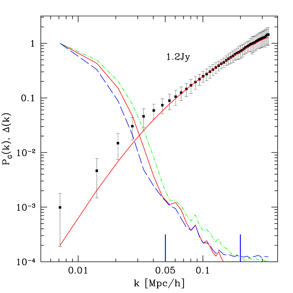
where $\bar{n}({\mathchoice{{\hbox{\BFd x}}}{{\hbox{\BFt x}}}{{\hbox{\BFs x}}}{{\hbox{\BFss x}}}})=\mathop{{}{\langle}{}}n_{g}({\mathchoice{{\hbox{\BFd x}}}{{\hbox{\BFt x}}}{{\hbox{\BFs x}}}{{\hbox{\BFss x}}}})\mathop{{}{\rangle}{}}$, $P_{F}(k)$ and $P_{G}(k)$ are the power spectra of the fields $F$ and $G({\mathchoice{{\hbox{\BFd x}}}{{\hbox{\BFt x}}}{{\hbox{\BFs x}}}{{\hbox{\BFss x}}}})\equiv w_{k}({\mathchoice{{\hbox{\BFd x}}}{{\hbox{\BFt x}}}{{\hbox{\BFs x}}}{{\hbox{\BFss x}}}})\bar{n}({\mathchoice{{\hbox{\BFd x}}}{{\hbox{\BFt x}}}{{\hbox{\BFs x}}}{{\hbox{\BFss x}}}})$. For IRAS surveys, $P_{G}(k)$ decays quite strongly with k, as seen in Fig. 6 for QDOT-PSCz (dashed), 1.2Jy (solid) and 2Jy (dot-dashed), where we assumed for definiteness $w_{k}({\mathchoice{{\hbox{\BFd x}}}{{\hbox{\BFt x}}}{{\hbox{\BFs x}}}{{\hbox{\BFss x}}}})=1/(1+n({\mathchoice{{\hbox{\BFd x}}}{{\hbox{\BFt x}}}{{\hbox{\BFs x}}}{{\hbox{\BFss x}}}})P_{0})$ with $P_{0}=2000$. As a first approximation we can thus treat $P_{G}(k)$ as a delta function, and we obtain the power spectrum and bispectrum estimators (Matarrese et al. 1997)

$$\hat{P}(k)=\frac{P_{F}(k)}{I_{22}}-(1+\alpha)\frac{I_{12}}{I_{22}},,$$ (44)

$$\hat{B}_{123}=\frac{B_{F}}{I_{33}}-(\hat{P}_{1}+\hat{P}_{2}+\hat{P}_{3})\frac{I_{23}}{I_{33}}-(1-\alpha^{2})\frac{I_{13}}{I_{33}},,$$ (45)

where $I_{ab}\equiv\int d^{3}x\ \bar{n}^{a}({\mathchoice{{\hbox{\BFd x}}}{{\hbox{\BFt x}}}{{\hbox{\BFs x}}}{{\hbox{\BFss x}}}})w_{k_{1}}({\mathchoice{{\hbox{\BFd x}}}{{\hbox{\BFt x}}}{{\hbox{\BFs x}}}{{\hbox{\BFss x}}}})\ldots w_{k_{b}}({\mathchoice{{\hbox{\BFd x}}}{{\hbox{\BFt x}}}{{\hbox{\BFs x}}}{{\hbox{\BFss x}}}})$ and $\alpha$ denotes the additional shot noise correction due to the use of a random catalog. In the volume limited case, $I_{ab}=\bar{n}^{a}$ and Eqs. (44-45) reduce to the standard shot noise correction results for $\alpha=0$, $\hat{P}=P-\bar{n}^{-1}$, $\hat{B}=B-\bar{n}^{-1}\sum_{i}\hat{P}_{i}-\bar{n}^{-2}$ (Peebles 1980). The estimator of the reduced bispectrum is thus

$$\hat{Q}_{123}=\frac{\hat{B}_{123}}{\hat{P}_{1}\hat{P}_{2}+\hat{P}_{2}\hat{P}_{3}+\hat{P}_{3}\hat{P}_{1}}.$$ (46)

Note that this involves a non-linear combination of estimators, so it is not necessarily and unbiased estimator of $Q$, as we shall discuss in the next section.

7 Effects of Survey Geometry and Sampling

7.1 Power Spectrum

Using Eq. (44) for the power spectrum, we find the recovered power spectrum shown in symbols in Fig. 6. The mean is obtained from 785 1.2Jy mock surveys, and the error bars correspond to the errors scaled to a single realization. The solid line shows the actual power spectrum in redshift space obtained from 200 2LPT realizations of $\Lambda$CDM, $\sigma_{8}=0.7$ (error bars on these measurements are supressed for clarity, they are completely negligible). We see from Fig. 6 that the convolution with the window of the survey $P_{G}(k)$ in Eq. (43) affects the recovery of the density power spectrum at scales $k<0.05$ h/Mpc. For $k>0.05$ h/Mpc, which are the scales we use in this work, the recovered power spectrum in the narrow-window approximation agrees very well with the correct answer.

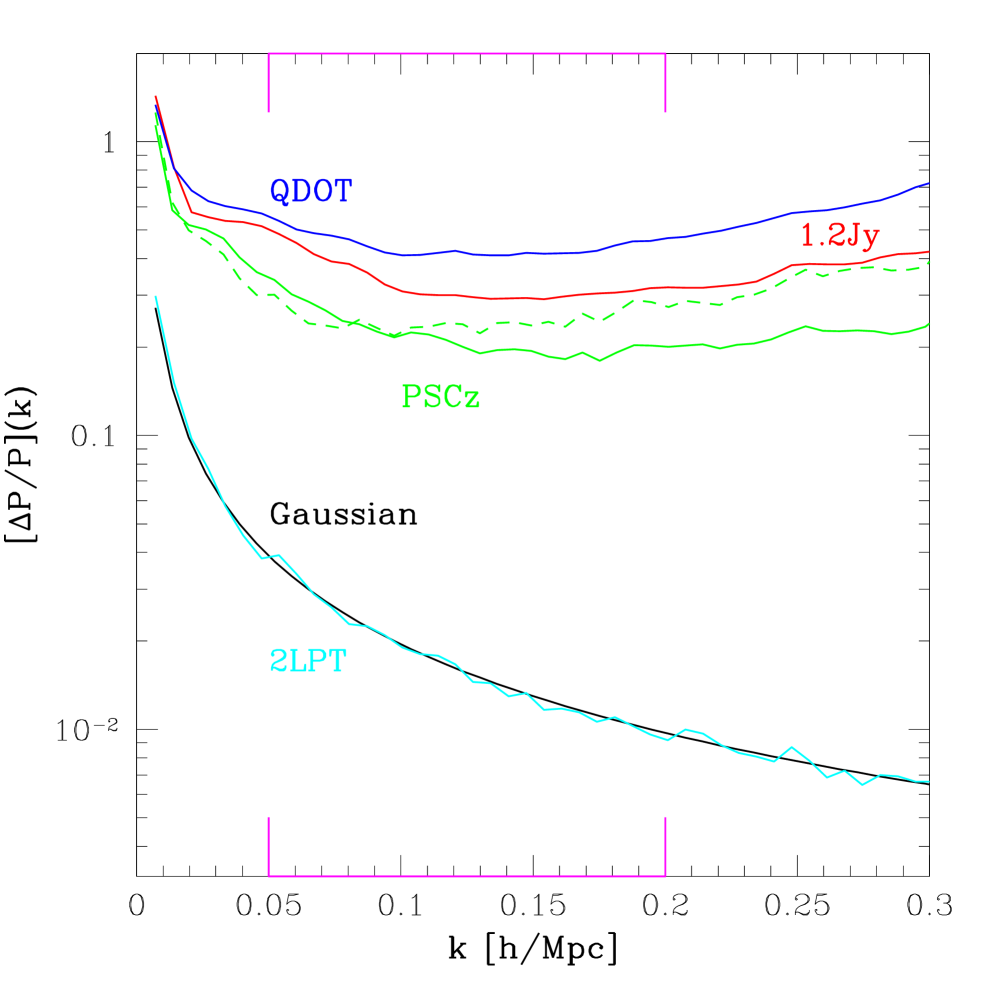
Figure 7 shows a comparison of the error bars as a function of scale in the ideal case (2LPT) with those in different IRAS surveys. Note that the horizontal scale is now linear, to show better the range of scales we actually use in this paper, and where the narrow-window approximation works. The 2LPT realizations are the same as in the previous figure, having $256^{3}$ particles in a 1200 Mpc/h box. The Gaussian prediction shown in Fig. 7 is obtained by the simple relation $\Delta P(k)/P(k)=2/N(k)$, where $N(k)$ is the number of modes within a given shell in Fourier space centered at $k$. From this comparison, we see that even at $k=0.3$ h/Mpc, the Gaussian approximation to the errors works very well, consistent with the results from N-body simulations in Meiksin & White (1999) and Scoccimarro, Zaldarriaga & Hui (1999).

Also shown in Fig. 7 are the corresponding errors for QDOT, 1.2Jy and PSCz surveys (those of 2Jy are intermediate between QDOT and 1.2Jy and are supressed for clarity). All the solid lines correspond to using the FKP weighing $P_{0}=2000$, constant for all wavenumbers. The dashed lines show the resulting error bars in PSCz mock surveys when $P_{0}=8000$. As expected, the error bars in the surveys are considerably larger than in the 2LPT case, due to the smaller volume and the larger shot noise. In fact, when the latter dominates, errors stop decreasing as $k$ is increased, which happens first for QDOT, then 1.2Jy and last for PSCz, as expected. The errors in the PSCz case are smaller for $P_{0}=8000$ at low $k$ than for $P_{0}=2000$ as expected, if one wants to measure longer wavelengths it is better to weight distant galaxies more (higher $P_{0}$), as dictated by the FKP prescription.

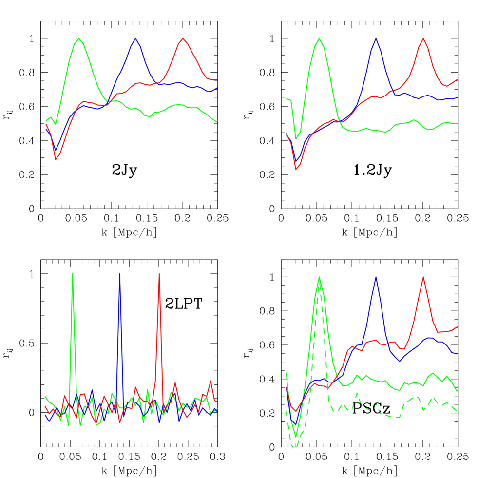
The survey geometry and sparse sampling (shot noise) not only increases the power spectrum error bars at a given $k$, but also leads to correlations between different band powers. To quantify this, Fig. 8 shows the power spectrum correlation coefficient, obtained from the power spectrum covariance matrix, $C_{ij}\equiv\mathop{{}{\langle}{}}(\hat{P}_{i}-P_{i})(\hat{P}_{j}-P_{j})\mathop{{}{\rangle}{}}$, by $r_{ij}\equiv C_{ij}/\sqrt{C_{ii}C_{jj}}$, for fixed $k_{i}$ as a function of $k_{j}$. The figure shows $k_{i}=0.053,0.134,0.201$ h/Mpc for different IRAS surveys and the “ideal” 2LPT case. In the latter (bottom left panel) we see that $r_{ij}$ is practically diagonal, no significant correlations are induced at these scales by non-linear evolution or the radial nature of redshift distortions. On the other hand, the 2Jy shows the slowest decay of $r_{ij}$, as expected due to its small volume. At the large $k$ end, $r_{ij}$ becomes roughly constant, when shot noise is expected to dominate the covariance between modes. All the mock survey results in this figure assume FKP weighing $P_{0}=2000$, except for the dashed line in the PSCz case (bottom right panel), which corresponds to $P_{0}=8000$. The larger value of $P_{0}$ in this case means that we are effectively increasing the volume of the survey, and thus the amount of cross-correlation between different band powers decreases. Thus, given the choice between $P_{0}=2000$ and $P_{0}=8000$ at $k\approx 0.1$ h/Mpc where both weights give similar error bars (see Fig. 7), the choice $P_{0}=8000$ should be preferred to decrease cross-correlations (which the FKP method does not attempt to minimize). In general, cross-correlation between different band powers are not negligible and must be taken into account when extracting cosmological information from power spectrum measurements (Eisenstein & Zaldarriaga 1999; Hamilton 2000; Hamilton & Tegmark 2000).

When estimating the power spectrum using likelihood analysis, an assumption must be made about the likelihood function. At large scales, the density field can be assumed to be Gaussian, and the power spectrum appears in the covariance matrix of the Fourier modes. At scales where non-linear effects become important, $k\approx 0.2-0.3$ h/Mpc, the density field cannot be assumed to be Gaussian anymore. A complementary approach at these scales is to consider that the power spectrum distribution about its mean is Gaussian; if there are enough independent modes contributing to a given shell in Fourier space, by the central limit theorem the distribution of the power spectrum should approach Gaussianity. However, due to the finite volume of the survey and shot noise, different modes are correlated, so it is not clear a priori at what scales Gaussianity applies. Figure 9 shows the power spectrum probability distribution function (PDF) obtained from 785 realizations of the 1.2Jy survey. The PDF is plotted as a function of the standarized variable $\delta P/\Delta P$, where $\delta P\equiv\hat{P}-P$, $\mathop{{}{\langle}{}}\hat{P}\mathop{{}{\rangle}{}}=P$, and $(\Delta P)^{2}\equiv\mathop{{}{\langle}{}}(\hat{P}-P)^{2}\mathop{{}{\rangle}{}}$. The four curves show the average power spectrum PDF for $k<0.067$, $0.067<k<0.134$, $0.134<k<0.201$, and $0.201<k<0.268$ (all in units of h/Mpc). The solid line denotes a Gaussian distribution, the actual distribution of power is approximately a $\chi^{2}$ distribution (with a number of degrees given by the effective number of modes one would obtain from Fig. 7 by assuming $\Delta P/P\approx 2/N_{\rm eff}(k)$) and becomes closer to Gaussian at small scales, as expected. We see though that at $k=0.268$ h/Mpc there are still noticeable deviations from Gaussianity.

7.2 Bispectrum

7.2.1 Choice of Triangle Variables

We now turn to a discussion of the bispectrum in mock surveys, focusing on the same issues illustrated by the power spectrum results discussed so far. For each realization of a given survey, the bispectrum is measured for all triangles with sides between $k=0.05$ h/Mpc and $k=0.2$ h/Mpc. The lower bound is imposed by the scale where the narrow-window approximation works well, whereas the upper bound is where shot noise can be best corrected for in a single realization, still well within the limits of applicability of 2LPT. The triangles are binned in terms of their sides, $k_{1}\geq k_{2}\geq k_{3}$, in steps of $k_{f}$, i.e. $k_{i}=10,11,12,...$, where $k_{f}$ is the “fundamental” mode of the Fourier space grid we use, $k_{f}=2\pi/1200\approx 0.005$ h/Mpc. There are 4741 such triangles in total, each of these triangles in turn contains from $10^{4}$ to $4\times 10^{6}$ “elementary” triangles (those involving the product of 3 Fourier coefficients).

Since the window function of the survey has a width of order $\Delta k/k_{f}\approx 5$ (see Fig. 6), triangles are very correlated if their sides differ by less than this width, as a result the number of “independent” triangles is of course much smaller than 4741. We therefore use coarser bins, defined in terms of shape $s$, ratio $r$, and scale $k$ parameters (Peebles 1980),

$$s\equiv\frac{k_{1}-k_{2}}{k_{3}},\qquad r\equiv\frac{k_{2}}{k_{3}},\qquad k\equiv k_{3},$$ (47)

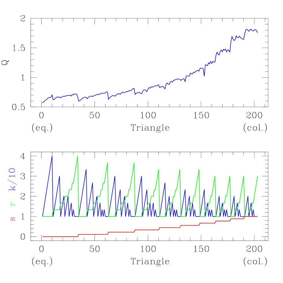
where the “shape” parameter $s$ obeys $0\leq s\leq 1$ ($k_{1}\geq k_{2}\geq k_{3}$), the ratio $1\leq r\leq 4$, and the overall scale of the triangle satisfies $10\leq k/k_{f}\leq 40$. The shape parameter is $s=0$ for isosceles triangles (and if $r=1$ these are equilateral triangles); for $s=1$ we have colinear triangles. Using 10 bins in each variable plus the closed triangle constraint yields 203 triangles.

One advantage of using these variables is that the main dependence of $Q$ is on the shape parameter $s$, with a small dependence on the ratio parameter $r$, and for a scale-free initial power spectrum no dependence on $k$. Therefore, if we plot $Q$ as a function of a single variable (“triangle”) which depends on ordered triplets ${s,k,r}$ as shown in the bottom panel of Fig. 10, $Q$ is roughly an increasing function of triangle number, which runs from 1 to 203. The order within the triplet is chosen so $s$ has the slowest variation, which means that low triangle number corresponds to nearly equilateral triangles, whereas high triangle number corresponds to nearly colinear triangles. For example, triangle number $1-10$ corresponds to equilateral triangles of scales $k/k_{f}=10,\ldots,40$. The top panel in Fig. 10 shows the reduced bispectrum $Q$ as a function of triangle number for 2LPT realizations in redshift-space of $\Lambda$CDM, with $\sigma_{8}=0.7$. This scheme of using a single (somewhat complicated) variable that parametrizes $Q$ will be useful in the following since it allows to deal with all the data at once (i.e. plot all the triangles of different shapes and scales in terms of a single variable).

7.2.2 Estimator Bias

The effects of finite volume on higher-order statistics has been well studied for one-point moments, in both N-body simulations (Colombi, Bouchet & Schaeffer 1994, 1995; Colombi, Bouchet & Hernquist 1996; Munshi et al. 1999) and galaxy surveys (Szapudi & Colombi 1996; Colombi, Szapudi & Szalay 1998; Kim & Strauss 1998; Hui & Gaztañaga 1999; Szapudi, Colombi & Bernardeau 1999). Here we consider the same problem for three-point statistics, i.e. the bispectrum.

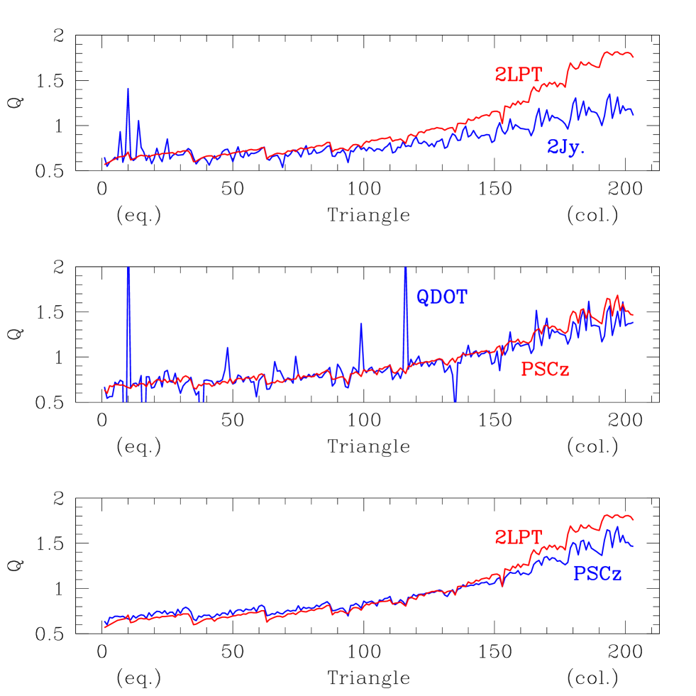
Figure 11 shows a comparison of the amplitude of the reduced bispectrum $Q$ as a function of triangle for different surveys and the underlying bispectrum (labeled 2LPT), to illustrate the effects of finite survey volume and sparse sampling. The top panel shows a comparison of 2LPT with 2Jy mock surveys, we see that the effects of finite volume (2Jy being the most shallow of the IRAS surveys) are rather strong: colinear configurations can be underestimated by factors as large as $70\%$. On the other hand, for the deeper PSCz survey (bottom panel) the finite volume effect is as expected substantially smaller, at about $20\%$. The middle panel compares the QDOT and PSCz surveys, the former being a sparse sample (one in six galaxies) of the latter. As we see, apart from a significant increase in the error bars, sparse sampling does not significantly affect the amplitude of the reduced bispectrum $Q$ (provided of course that the discretness corrections in Eqs. (44-45) can be performed accurately), except perhaps by factors of order $10\%$ at colinear configurations.

The finite volume effect is particularly worrisome for the determination of galaxy bias parameters from surveys, as it has a similar systematic effect on $Q$ as galaxy biasing with $b_{1}>1$ and $b_{2}>0$. For example, if this effect is ignored, one would conclude erroneously from the unbiased realizations (i.e. $b_{1}=1$, $b_{2}=0$) in Fig. 11 that $b_{1}=2.23,1.35$ and $b_{2}=2.18,0.42$ for 2Jy and PSCz respectively. This “estimator bias”, the fact that the estimator of $Q$ is not unbiased, arises because $\hat{Q}_{123}$ in Eq. (46) is a non-linear combination of estimators, which are nonetheless unbiased (provided that we use the mean value of the selection function, rather than its actual value to substract the mean density, and thus avoid the integral constraint bias). There are two sources of estimator bias in Eq. (46) corresponding to the two non-linear operations involved; the quadratic combination in the denominator of Eq. (46) and the ratio between numerator and denominator. Detailed analysis shows that both contributions turn out to be important, in particular, the quadratic combination overestimates the underlying value (obtained from 2LPT) for colinear configurations (thus leading to an understimate of $Q$ for these triangles), whereas taking the ratio also leads to an underestimate of $Q$ for colinear configurations. In addition, there is a rather small overestimate of $Q$ for equilateral configurations (only apparent in the least noisy PSCz mock surveys, bottom panel of Fig. 11). This however can be traced to a small estimator bias in the bispectrum for equilateral triangles at large scales, which indicates that the narrow window approximation used to deconvolve with the survey window bispectrum in Eq. (45) is beginning to break down. However, the effect of this particular estimation bias is in practice negligible when compared to the other estimation biases involved.

7.2.3 Error Bars and Triangle Cross-Correlations

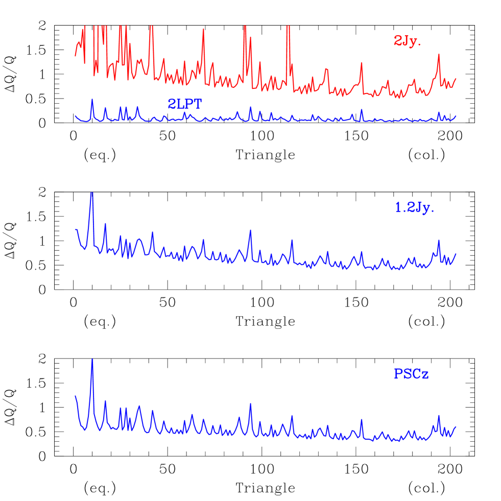
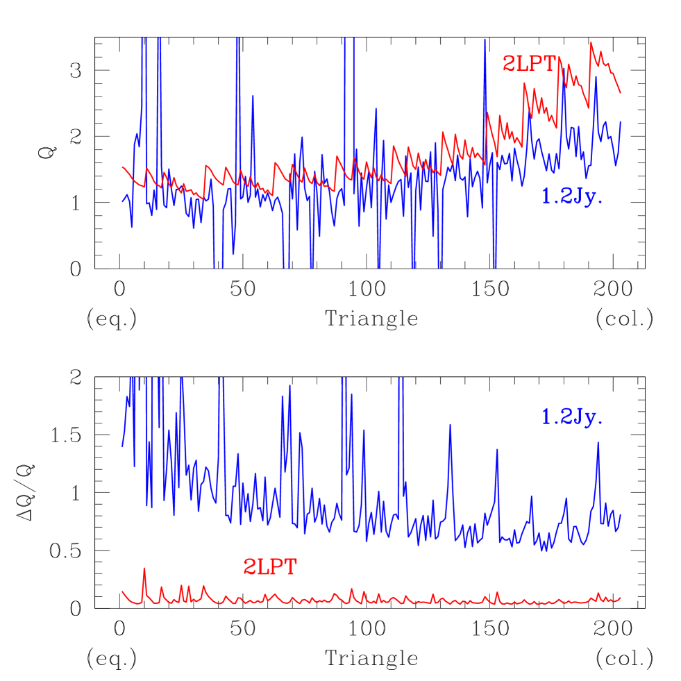
Figure 12 shows the relative error on the reduced bispectrum, $\Delta Q/Q$ as a function of triangle for different surveys, where $(\Delta Q)^{2}\equiv\mathop{{}{\langle}{}}(Q-\bar{Q})^{2}\mathop{{}{\rangle}{}}$. The top panel shows the ideal 2LPT case, and the errors expected in a single realization of the 2Jy survey. Similarly, the middle and bottom panels show the corresponding results for 1.2Jy and PSCz surveys. We see that in general errors decrease as configurations become more colinear (simply because the number of triangles increases), with spikes due to shot noise at small scales. For example, the spike at the tenth triangle is due to equilateral triangles at small scales ($k=0.2$ h/Mpc) becoming dominated by shot noise. For QDOT (not shown), $\Delta Q/Q>1$ for all triangles, with most triangles having significantly larger errors. In Fig. 13, we show similar results for $\chi^{2}$ initial conditions. The 2LPT results are from Scoccimarro (2000), and the 1.2Jy results show the rather strong finite volume effects (top panel) and the increase error bars with respect to the Gaussian initial conditions case (compare with middle panel in Fig. 12). These results are noiser than in the Gaussian case shown in Figs. 11-12 because only 200 (instead of $\approx 10^{3}$) mock catalogs are used to compute $Q$ and $\Delta Q$.

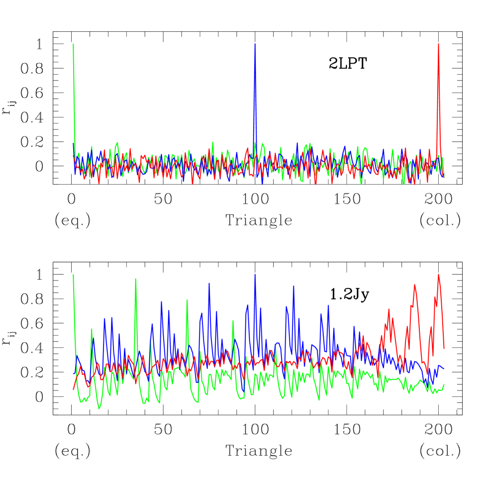
Figure 14 shows the bispectrum correlation coefficient, obtained from the covariance matrix as in the power spectrum case. This measures correlations between different triangles and shows that in the ideal case (2LPT, top panel) different triangles are practically independent, whereas when survey geometry and sampling are included (1.2Jy, bottom panel), correlations between different triangles are significant. The peaks in the correlation coefficient can be matched with triangles that have their sides of similar length, as expected from the power spectrum correlations shown in Fig. 8.

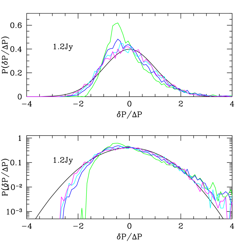
7.2.4 The Distribution of $Q$

The main ingredient to implement a likelihood analysis is to understand the probability distribution (PDF) of the reduced bispectrum $Q$. In order to do that, we use the 2LPT Monte Carlo realizations to construct the PDF’s for different mock surveys. As found for the power spectrum (Fig. 9), we expect that bispectrum correlations due to survey geometry and sampling as shown in Fig. 14 invalidate straightforward application of the central limit theorem, and thus convergence to a Gaussian distribution for $Q$.

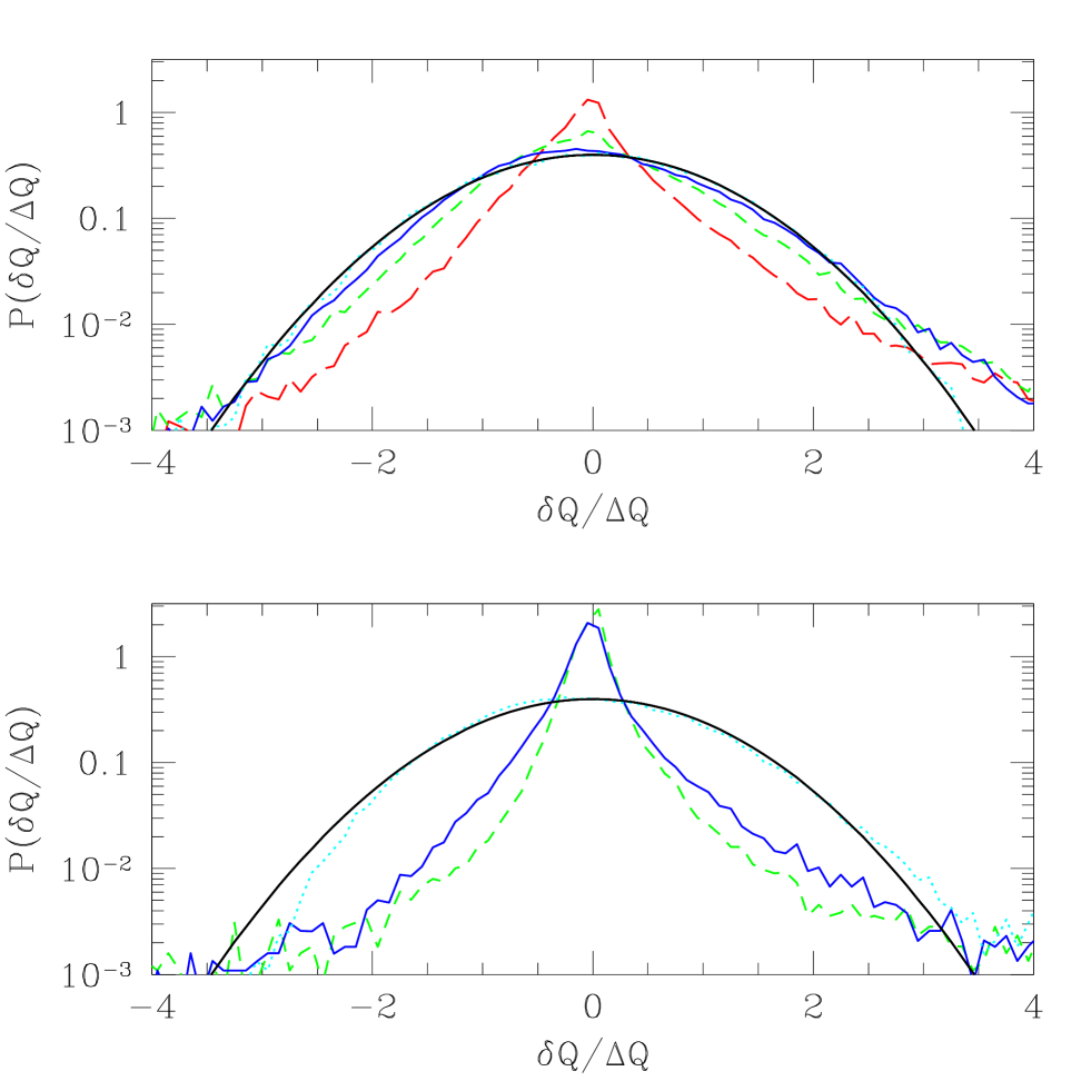
Figure 15 shows the results. We found that the distributions of $Q$ for all the triangles we consider were very similar when plotted in terms of the scaled variable $\delta Q/\Delta Q$, where $\delta Q\equiv Q-\bar{Q}$. We have thus averaged all these PDF’s to increase the signal to noise. In reality one expects these PDF’s to approach Gaussianity when the error is small (i.e. survey geometry and sampling are not significant), and thus a variation of PDF on scale; however for the range of scales we consider the errors don’t change significantly (see Fig. 12), so to first approximation the PDF’s do not change.

The dotted lines in the top panel of Fig. 15 shows indeed that in the ideal case (2LPT) the PDF of $Q$ approaches Gaussianity (solid smooth line). On the other hand, mock surveys show clear deviations from Gaussianity, with positive skewness, exponential tails for 1.2Jy and 2Jy surveys, and in the sparse sampling case (QDOT) power-law tails and rather strong kurtosis. For $\chi^{2}$ non-Gaussian initial conditions (bottom panel), the non-Gaussianity is even more pronounced, as expected. This clearly shows that likelihood analysis for current surveys based on a Gaussian likelihood for the bispectrum are not justified. In particular, the skewness of the PDF can lead to a “statistical” bias in the estimation of galaxy bias: since the most likely value for $Q$ is to underestimate the mean, use of a Gaussian likelihood will infer bias parameters that overestimate $b_{1}$ and understimate $b_{2}$.

8 Likelihood Analysis

8.1 $Q$ Eigenmodes

A general treatment of likelihood non-Gaussianity and cross-correlations between triangles is very complicated. Here we will make the assumption that the eigenmodes of $Q$, defined by diagonalizing its covariance matrix, are effectively independent (which would be true if their joint PDF were Gaussian), and thus write the full likelihood as a product of eigenmode-likelihoods (which are computed by 2LPT realizations of a given survey, and are generally non-Gaussian). In general, diagonalizing the covariance matrix does not guarantee that the eigenmodes are independent (third and higher-order correlations could be still non-zero), but as we shall see this simplification seems to work very well in practice.

Given a set of measured reduced bispectrum amplitudes $\{Q_{m}\}$, $m=1,\ldots,N_{T}$, where $N_{T}$ is the number of closed triangles in the survey, we diagonalize their covariance matrix so the $Q$-eigenmodes $\hat{q}_{n}$,

$$\hat{q}_{n}=\sum_{m=1}^{N_{T}}\gamma_{mn}\ \frac{Q_{m}-\bar{Q}_{m}}{\Delta Q_{m}},$$ (48)

satisfy

$$\mathop{{}{\langle}{}}\hat{q}_{n}\hat{q}_{m}\mathop{{}{\rangle}{}}=\lambda_{n}^{2}\,\delta_{nm},$$ (49)

where $\bar{Q}\equiv\mathop{{}{\langle}{}}Q\mathop{{}{\rangle}{}}$ and $(\Delta Q)^{2}\equiv\mathop{{}{\langle}{}}Q^{2}\mathop{{}{\rangle}{}}-\bar{Q}^{2}$. These $Q$-eigenmodes have “signal to noise” ratio $S/N$,

$$\left(\frac{S}{N}\right)_{n}\equiv\frac{1}{\lambda_{n}}\,\left|\sum_{m=1}^{N_{T}}\gamma_{mn}\,\frac{\bar{Q}_{m}}{\Delta Q_{m}}\right|.$$ (50)

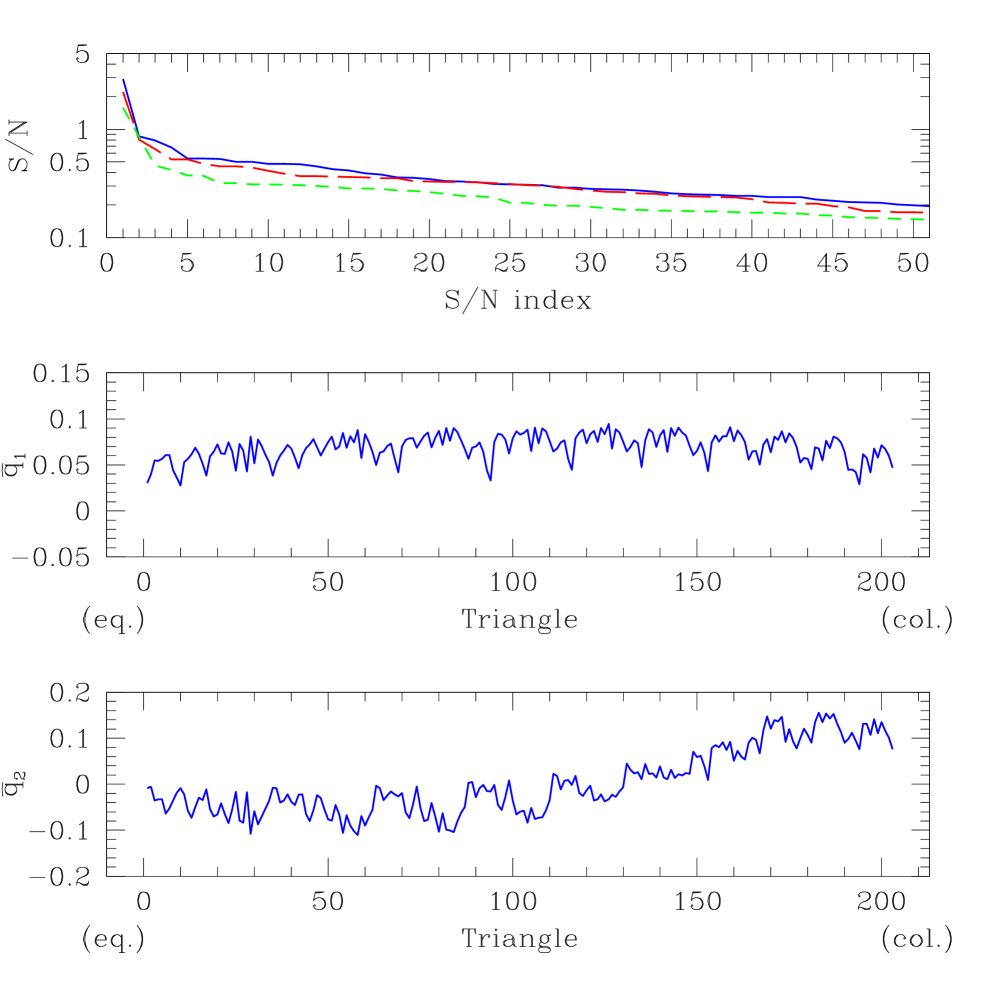
The physical interpretation of $Q$-eigenmodes becomes clear when ordered in terms of their signal to noise, as shown in the top panel in Fig. 16. The best eigenmode (highest signal to noise, $S/N\approx 3$), say $n=1$, corresponds to all weights $\gamma_{m1}>0$; that is, it represents the overall amplitude of the bispectrum (Fig. 16, middle panel). The next $Q$-eigenmode, $n=2$ with $S/N\approx 1$, has $\gamma_{m2}>0$ for nearly colinear triangles and $\gamma_{m2}<0$ for nearly equilateral triangles (Fig. 16, bottom panel); that is, it represents the configuration dependence of the bispectrum. Higher-order eigenmodes contain further information such as variations of amplitude and shape with scale, but generally have $S/N<1$ in IRAS catalogs (although there are many of them). The $S/N$ of eigenmodes for a particular survey is sensitive mostly to the biasing scheme and the amplitude of fluctuations $\sigma_{8}$, stronger clustering leading to larger $S/N$ overall.

8.2 Recovering Bias Parameters

As discussed above, we can write down the likelihood as a function of the bias parameters,

$${\cal L}(\alpha_{1},\alpha_{2})\propto\prod_{i=1}^{N_{T}}P_{i}[\nu_{i}(\alpha_{1},\alpha_{2})],$$ (51)

where $\alpha_{1}\equiv 1/b_{1}$, $\alpha_{2}\equiv b_{2}/b_{1}^{2}$, and

$$\nu_{i}(\alpha_{1},\alpha_{2})\equiv\frac{1}{\lambda_{i}}\ \sum_{j=1}^{N_{T}}\gamma_{ji}\,\frac{Q_{j}-(\alpha_{1}\bar{Q}_{j}+\alpha_{2})}{\Delta Q_{j}},$$ (52)

where the $Q_{j}$ ($j=1,\ldots,N_{T}$) are the data, and the mean $\bar{Q}_{j}$, standard deviation $\Delta Q_{j}$, and the non-Gaussian PDF’s $P_{i}(\nu_{i})$ are extracted from the mock catalogs. Essentially, the $Q$-eigenmode PDF’s look similar to those shown in Fig. 15 for $n=1$ (for which $\gamma_{m1}>0$), and a symmetrized version of it for other eigenmodes where $\gamma_{mn}$ takes positive and negative values equally frequent. We assume that to first approximation, $\Delta Q_{j}$ does not depend on biasing, which would be true if biasing is linear and deterministic. Thus, in the following all results shown ignore a possible dependence of $\Delta Q_{j}$ on non-linear biasing.

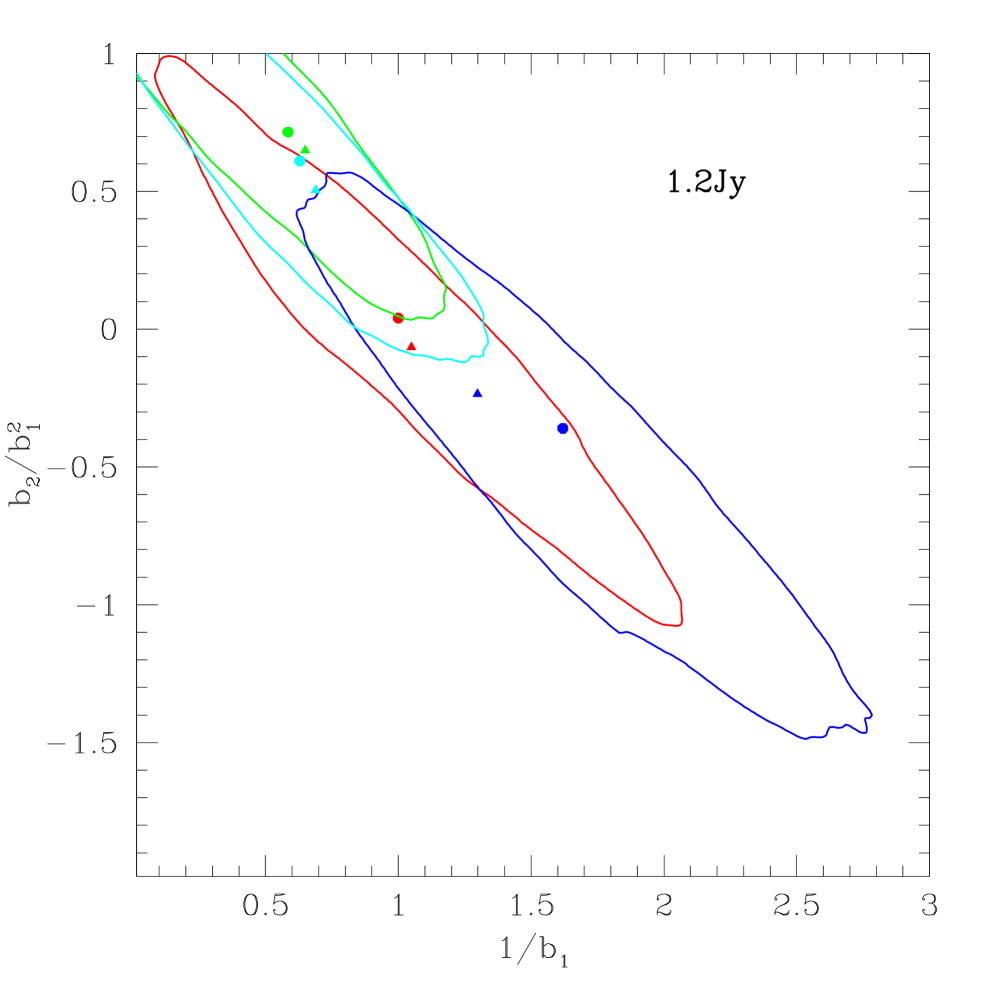
Figure 17 shows an example of the use of Eq. (51) to recover bias parameters. We use parent 2LPT realizations of $200^{3}$ particles in a 600 Mpc/h box, which are then used to select about $2\times 10^{6}$ “galaxies” according to the prescription in Eq. (14). These realizations are then used to generate mock catalogs of the 1.2Jy survey. We generated 200 mock catalogs for each of the biasing schemes shown in Fig. 1, and then measure $Q$ in redshift space. Three of the models are generated from $\Lambda$CDM ($\sigma_{8}=0.7$, $\Omega_{m}=0.3$, $\Omega_{\Lambda}=0.7$) and a fourth model with same power spectrum shape and normalization but $\Omega_{m}=1$ (top right panel). The models in the right panels have about the same $\beta\equiv\Omega_{m}^{0.6}/b_{1}\approx 0.65$. We now describe the results of analyzing these biased samples with the likelihood in Eq. (51) where all the quantities ($P_{i},\bar{Q}_{j},\Delta Q_{j}$) are evaluated from the unbiased ($b_{1}=1$, $b_{2}=0$) realizations of the surveys described above to test the assumptions behind our likelihood analysis.

The plots in Fig. 17 show typical outcomes of the maximum likelihood procedure; triangles denote the “correct” biasing parameters shown in Fig. 1 (obtained by measuring the bispectrum in the parent 2LPT realization). The best fit parameters and error bars from these particular single realizations of biased catalogs are shown in Table 6. Note that, as expected, the derived error bars increase for the antibiased samples. It is also important to note that although the bispectrum can break the degeneracy between models with the same $\beta$ but different bias and $\Omega_{m}$, for the 1.2Jy survey the errors are large enough that the two models considered overlap to within $68\%$. These results are only meant to illustrate the expected error bars and do not constitute a test of the likelihood analysis (since one can always find a single realization out of 200 which shows reasonable reconstruction of the biasing parameters). To test the accuracy of the likelihood analysis, we checked whether $68\%$ likelihood ellipses enclosed the correct answer in $68\%$ of the realizations. We found that in practice this number is about $70\%$; if we instead use a Gaussian likelihood (including correlations) we found that this number drops to about $45\%$. Correlations between triangles account for a significant area of the ellipses in Fig. 17, neglecting correlations leads to error ellipses that contract by a factor of order 10 in area.

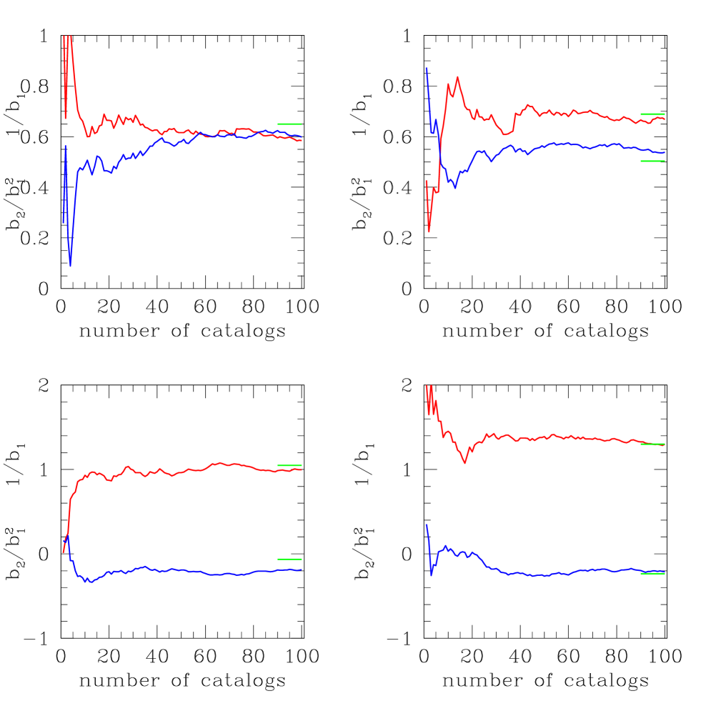
The use of maximum likelihood (ML) to estimate the best fit bias parameters is not guaranteed to give statistically unbiased results, since the likelihood is not Gaussian. To test this, Fig. 18 shows the ML estimates as a function of the cumulative number of mock catalog realizations used, with panels ordered as in Fig. 1. The deviations observed at low numbers of catalogs is due to the effect discussed above, i.e. one expects individual realizations which are off the underlying value (error bars for each curve in Fig. 18 are avoided for reasons of clarity, but can be estimated from the ones in Table 6 by scaling by $1/\sqrt{N_{\rm cat}}$). We see that as the number of catalogs $N_{\rm cat}$ becomes large (and the error bars become small), the results generally approach the expected asymptotic value of $1/b_{1}$, $b_{2}/b_{1}^{2}$ (shown as horizontal marks in Fig. 18; see also Fig. 1 and Table 6). However, there are detectable (small) estimation biases, in particular for the non-linear bias parameter. For the lower left panel, the resulting parameters actually make the agreement in Fig. 1 better. Since these estimation biases are about $3-4$ times smaller than the expected error bars for a single survey, we can safely ignore this problem, as it appears not to be systematic. For larger surveys, where the errors are expected to be smaller it is also expected that the likelihood will be better approximated by a Gaussian, thus the estimation bias from ML is also likely to be smaller, so it is not clear this is a serious problem for constraining bias parameters, but it is worth keeping in mind.

8.3 Comparison with Previous Work

A likelihood analysis for obtaining bias parameters from bispectrum measurements has been pioneered by Matarrese et al. (1997; MVH), and extended to redshift-space by Verde et al. (1998). Their approach differs from ours in several ways, as they intended their treatment to next-generation redshift surveys where some of issues faced in this work will not be as serious (although this will have to be checked in each particular case). First, they assume a Gaussian likelihood for the bispectrum, which as discussed above breaks down in the case of IRAS surveys. This approximation will considerably improve for surveys such as 2dF and SDSS.

Second, we consider all triangle shapes with their full covariance matrix, rather than using only equilateral and colinear triangles to make the covariance approximately diagonal. In fact, for IRAS surveys Fig. 14 shows that triangles of similar shapes and scales are strongly correlated by the window of the survey and sparse sampling. In addition, discarding triangle shapes throws away information, which is undesirable. This is of course not a limitation of MVH’s method; on the other hand, analytic calculation of the covariance matrix between general triangle shapes including the effects of survey geometry and sampling quickly becomes complicated if one intends to go beyond the Gaussian approximation. In our case this is handled automatically by the numerical 2LPT realizations.

Our treatment of perturbation theory (PT) leads to some minor improvements. By being Lagrangian, our calculation includes loop corrections beyond leading order, although only approximately. Their treatment using second-order Eulerian PT is only consistent for the bispectrum, not its covariance (which has contributions from the sixth-point function and thus requires fifth-order Eulerian PT); however the leading order contribution is Gaussian, so to leading order (most of the contribution at the scales of interest) both treatments should agree. 2LPT is not exact beyond second-order in Eulerian space, however the results of Table 2 show that it gives a very good approximation to the higher-order moments.

The most important difference is the treatment of redshift distortions, our numerical calculations allow us to perform the redshift-space mapping exactly (rather than perturbatively), which makes quantitative difference even at large scales (e.g. solid versus dotted lines in Fig. 3). Moreover, by using non-linear dynamics rather than a phenomenological model to treat non-linear distortions, we avoid introducing auxiliary quantities such as the velocity dispersion parameter $\sigma_{v}$ (Verde et al. 1998; Scoccimarro et al. 1999).

Our calculations of the finite volume effects are in reasonable agreement with the results found for one-point higher-order statistics (Szapudi et al. 1999a, 1999b). In particular, we find that the PDF of the bispectrum is generally non-Gaussian with positive skewness, whereas Szapudi et al. (1999b) find that the PDF of the skewness parameter $S_{3}$ can be approximated by a suitably scaled lognormal. We also find that in general the estimator bias for $Q$ is smaller than the error $\Delta Q$, although in the case of the 2Jy survey both quantities are comparable. It is thus important to correct for estimator bias (Hui & Gaztañaga 1999), even when it is smaller than the error, since the systematic shift affects the performance of the likelihood estimation; i.e. without this correction $68\%$ likelihood contours would not enclose the correct answer $68\%$ of the time. Our approach can be also applied to one-point statistics, and would be interesting to compare with the results by Szapudi et al. (1999a,1999b) since they involve different approximations.

9 Summary and Conclusions

We studied the use of the bispectrum to recover bias parameters and constrain non-Gaussian initial conditions in realistic redshift surveys. We considered the effects of stochastic non-linear biasing, radial redshift-distortions, survey geometry and sampling on the shape dependence of the bispectrum.

We found that bias stochasticity does not seem to affect the use of the bispectrum to recover the mean biasing relation between galaxies and mass, at least for models in which the scatter is uncorrelated at large scales. Clearly more work is necessary along these lines, we have just considered a very simple extension to the local deterministic bias model. We also found that the radial nature of redshift distortions changes the bispectrum monopole compared to the plane-parallel values by only a few percent, well below current error bars.

On the other hand, survey geometry leads to finite volume effects which must be taken into account in current surveys before comparison with theoretical predictions can be made. Similarly, sparse sampling and survey geometry correlate different triangles leading to a breakdown of the Gaussian likelihood approximation. We developed a likelihood analysis using bispectrum eigenmodes, calculated by Monte Carlo realizations of mock surveys generated with second-order Lagrangian perturbation theory (2LPT) and checked against N-body simulations. This can be used to derive quantitative constraints from current and future redshift surveys. In a companion paper (Scoccimarro et al. 2000) we apply the results obtained here to the analysis of the bispectrum in IRAS surveys.

Our treatment can be improved in several ways for applications to surveys that demand more accuracy. In particular, we relied on the simple relation in Eq. (3) to relate the galaxy bispectrum to the mass bispectrum; in practice, however, redshift-distortions and biasing do not conmute, and this relation is more complicated (Scoccimarro, Couchman & Frieman 1999). Related to this issue is a formulation, so far lacking, of a joint likelihood for the power spectrum and bispectrum, which involves dependence on $\Omega_{m}$ and biasing parameters. In addition, we have only considered closed triangles in Fourier space. In practice, due to breakdown of translation invariance by the survey geometry, selection function, and radial redshift distortions, open triangles also contain useful information. In order to do this, one possibility is to construct a general cubic estimator for the bispectrum, analogous to the quadratic estimator for the power spectrum (e.g. Tegmark et al. 1998), which seems a rather difficult task for non-Gaussian fields. However, future large redshift surveys such as 2dF and SDSS will be the ideal datasets to take full advantage of the cosmological information available from higher-order statistics, and thus the effort in developing more accurate statistical methods will likely be rewarded.

Table 1: Ratio $r_{p}$ of $S_{p}$ parameters ($3\leq p\leq 8$) in the ZA to their exact values as a function of spectral index $n$.

$n$	$r_{3}$	$r_{4}$	$r_{5}$	$r_{6}$	$r_{7}$	$r_{8}$
-3	0.82	0.66	0.52	0.41	0.32	0.25
-2	0.77	0.58	0.42	0.30	0.22	0.15
-1	0.70	0.45	0.28	0.17	0.10	0.06
0	0.54	0.25	0.10	0.04	0.01	0.006

Table 2: Ratio $r_{p}$ of $S_{p}$ parameters ($3\leq p\leq 8$) in 2LPT to their exact values as a function of spectral index $n$.

$n$	$r_{3}$	$r_{4}$	$r_{5}$	$r_{6}$	$r_{7}$	$r_{8}$
-3	1	0.98	0.95	0.92	0.89	0.86
-2	1	0.96	0.92	0.87	0.82	0.77
-1	1	0.93	0.84	0.74	0.65	0.57
0	1	0.80	0.54	0.35	0.24	0.17

Table 3: Ratio $r_{p}$ of $S_{p}$ parameters ($3\leq p\leq 8$) in 3LPT to their exact values as a function of spectral index $n$.

$n$	$r_{3}$	$r_{4}$	$r_{5}$	$r_{6}$	$r_{7}$	$r_{8}$
-3	1	1	0.99	0.99	0.99	0.98
-2	1	1	0.99	0.98	0.97	0.96
-1	1	1	0.98	0.95	0.92	0.88
0	1	1	0.89	0.74	0.56	0.41

Table 4: Percentage of shell-crossing grid points ($x_{sc}$) and ratios of second to first-order displacements as a function of power spectrum cutoff ($k_{c}$ in h/Mpc) for $\Lambda$CDM ($\sigma_{8}=0.7$) as in Fig. 2.

$k_{c}$	$x_{sc}$	$\left<|{\bf\Psi}_{2}|\right>/\left<|{\bf\Psi}_{1}|\right>$
0.3	1.80	0.19
0.4	7.32	0.23
0.5	14.89	0.26
$\infty$	42.15	0.32

Table 5: Selection function parameters (see Eq. (39)) for different IRAS mock catalogs.

Catalog	$A$	$r_{0}$	$a$	$b$
QDOT	2.42	86.01	0.52	2.98
2 Jy.	3.61	69.52	0.05	3.16
1.2 Jy.	7.87	72.65	0.43	3.28
PSCz	18.83	76.71	0.81	3.1

Table 6: Recovery of bias parameters from a single realization of the 1.2Jy survey with stochastic non-linear bias (likelihood contours shown in Fig. 17)

$1/b_{1}$ (2LPT)	$1/b_{1}$ (mock)	$b_{2}/b_{1}^{2}$ (2LPT)	$b_{2}/b_{1}^{2}$ (mock)
0.65	$0.59^{+0.42}_{-0.30}$	0.65	$0.71^{+0.28}_{-0.36}$
0.69	$0.63^{+0.46}_{-0.33}$	0.50	$0.61^{+0.31}_{-0.48}$
1.05	$1.00^{+0.61}_{-0.55}$	-0.07	$0.04^{+0.51}_{-0.67}$
1.30	$1.62^{+0.69}_{-0.60}$	-0.24	$-0.36^{+0.52}_{-0.79}$

Figure 1: Recovering stochastic non-linear bias from bispectrum measurements. The smooth solid line is the bias relation obtained from the bispectrum with parameters $b_{1}$ and $b_{2}$ as shown in each panel. The true bias relation is represented by the central line (mean) and the $90\%$ scatter around it. The smoothing scale is $R=10$ Mpc/h .

Figure 2: The top panel shows the power spectrum in redshift space as a function of scale for linear PT (dotted), 2LPT (solid), and N-body simulations (symbols). The bottom panel shows the reduced bispectrum for equilateral triangles in redshift space as a function of scale in tree-level PT (dotted), 2LPT (solid) and N-body simulations (symbols, with error bars from 4 different realizations).

Figure 3: The bispectrum in redshift space for configurations with $k_{2}=2k_{1}=0.21$ h/Mpc as a function of the angle $\theta$ between ${\mathchoice{{\hbox{\BFd k}}}{{\hbox{\BFt k}}}{{\hbox{\BFs k}}}{{\hbox{\BFss k}}}}_{1}$ and ${\mathchoice{{\hbox{\BFd k}}}{{\hbox{\BFt k}}}{{\hbox{\BFs k}}}{{\hbox{\BFss k}}}}_{2}$. Dotted lines denote tree-level PT, solid lines correspond to 2LPT, and symbols with error bars show the result of 4 realizations of N-body simulations.

Figure 4: The power spectrum in N-body simulations for $\Lambda$CDM (top set) and SCDM (bottom). Solid lines denote measurements in real space, whereas dotted lines and dashed lines (practically on top of each other) denote measurements in redshift space under radial mapping and in the plane-parallel approximation, respectively.

Figure 5: The top left panel shows the ratio of bispectra for radial to plane-parallel redshift-space mapping as a function of angle as in Fig. 4. Triangles denote $k_{2}=2k_{1}=0.105$ h/Mpc, squares $k_{2}=2k_{1}=0.21$ h/Mpc. The remaining panels show sensitivity of $Q$ to change in parameters: $\Omega_{m}$ (top right), $\sigma_{8}$ (bottom left), $\Gamma$ (bottom right).

Figure 6: Symbols with error bars (scaled to a single survey) denote the recovered power spectrum from $\Lambda$CDM realizations of the 1.2Jy survey. Band powers are correlated as shown in top right panel in Fig. 8. The overestimate at scales $k<0.05$ h/Mpc is due to ignoring the width of the survey window. The plot also shows the power spectrum of the survey window for 2Jy (dot-dashed), 1.2Jy (solid) and QDOT-PSCz (dashed).

Figure 7: Power spectrum error bars as a function of scale, for 2LPT, PSCz with $P_{0}=2000$ (solid) and $P_{0}=8000$ (dashed), 1.2Jy and 2Jy.

Figure 8: Power spectrum correlation coefficient, for 2Jy, 1.2Jy, PSCz ($P_{0}=2000$, solid), PSCz ($P_{0}=8000$, dashed) and 2LPT, as a function of scale.

Figure 9: Power spectrum PDF as a function of scale in linear (top) and logarithmic (bottom) scale, smooth solid line denotes a Gaussian distribution. From least to most non-Gaussian, scales are $k/k_{f}=1-10$, $k/k_{f}=11-20$, $k/k_{f}=21-30$, $k/k_{f}=31-40$, where $k_{f}=0.005$ h/Mpc.

Figure 10: the top panel shows $Q$ measured in the 2LPT realizations for all triangles, as a function of triangle shape in redshift space, for $\Lambda$CDM with real space $\sigma_{8}=0.70$. Bottom panel shows the parameters $s,r,k$ as a function of triangle number. Essentially, triangles start equilateral and become colinear as triangle number increases.

Figure 11: Comparison between underlying bispectrum (2LPT) and the bispectrum obtained in mock surveys, for 2Jy (top) and PSCz (bottom). The finite volume of the survey causes estimation bias. The middle panel shows a comparison between PSCz and QDOT to quantify the effects of sparse sampling.

Figure 12: Bispectrum error bars as a function of triangle for different surveys and 2LPT.

Figure 13: Same as previous two figures for $\chi^{2}$ initial conditions.

Figure 14: Bispectrum correlation coefficient, as a function of triangle for 2LPT (top) and 1.2Jy mock surveys (bottom).

Figure 15: PDF of $\delta Q/\Delta Q\equiv(Q-\bar{Q})/\Delta Q$ for different surveys in models with Gaussian (top) and $\chi^{2}$ non-Gaussian (bottom) initial conditions: 2LPT (dotted), IRAS 1.2Jy (solid), IRAS 2Jy (dashed), IRAS QDOT (long-dashed). The smooth solid curve is a Gaussian distribution.

Figure 16: The top panel shows the signal to noise of $Q$-eigenmodes [see Eq. (50)], with line styles as in Fig. 15. The remaining panels show the eigenfunctions for the best determined eigenmode ($\hat{q}_{1}$), sensitive to the overall amplitude of $Q$, and the the second best eigenmode ($\hat{q}_{2}$), which is most sensitive to the configuration dependence of $Q$.

Figure 17: Maximum likelihood estimation from stochastic non-linear bias realizations of the 1.2Jy survey, corresponding to those shown in Fig. 1. Contours are $68\%$, triangles denote the parameters shown in Fig. 1. The maximum likelihood values (circles) and marginalized error bars are shown in Table 6.

Figure 18: Maximum likelihood estimates of bias parameters as a function of number of 1.2Jy mock catalogs used. The horizontal marks on the right denote the values of $b_{2}/b_{1}^{2}$ and $1/b_{1}$ from a parent 2LPT realization as shown in Fig. 1.