Unbiased reconstruction of the mass function using microlensing survey data.

Abstract

The large number of microlensing events discovered towards the Galactic Bulge bears the promise to reconstruct the stellar mass function. The more interesting issue concerning the mass function is certainly to probe its low mass end, near the region occupied by the brown dwarfs. However due to the source confusion, even if the distribution and the kinematics of the lenses are known, the estimation of the mass function is extremely biased at low masses. The blending due to the source confusion biases the duration of the event, which in turn dramatically biases the estimation of the mass of the lens. To overcome this problem we propose to use differential photometry of the microlensing events obtained using the image subtraction method. Differential photometry is free of any bias due to blending, however the drawback of differential photometry is that the baseline flux is unknown. In this paper we will show that even without knowing the baseline flux, purely differential photometry allow to estimate the mass function without any biases. The basis of the method is that taking the scalar product of the microlensing light curves with a given function and taking its sum over all the microlensing events is equivalent to project the mass function on another function. This method demonstrates that there is a direct correspondancy between the space of the observations and the space of the mass function. Concerning the function to use in order to project the observations, we show that the principal components of the light curves are an optimal set. We also demonstrate that there is no additional information about the distribution of the scalar products of the data beyond their sum (first order moment). Higher order moments are only linear combination of the first order moment. Thus the sum of the projection on the principal components contains all the information, and translate in an equal number of projection of the mass function with functions associated with the principal components. To illustrate the method we simulate data sets consistent with the microlensing experiments. By using 1000 of these simulations, we show that for instance the exponent of the mass function can be reconstructed without any biases.

1 Introduction.

The success of the microlensing experiments has been impressive, several collaborations have reported the detection of microlensing amplification of stars, OGLE (Udalski et al. 2000), MACHO (Alcock et al. 1998), EROS (Derue et al. 1999)), DUO (Alard & Guibert 1997), VATT (Uglesich et al. 1999). In particular, the recent release by the OGLE II collaboration of more than 200 microlensing events is of great interest. One of the obvious promises of such data sets is the possibility to explore the mass function near the low mass end. Although, the relation between the mass function and the microlensing observations is not straightforward. In the classical scheme of analysis, one must first estimate the duration of the events by fitting the theoretical light curves, then compute the lensing rates, and finally relate these lensing rates to the mass function. The trouble is that fitting the theoretical light curve to the microlensing data to obtain the duration of the event is a highly degenerated process (Alard 1997, Han 1997, Wozniak & Paczyǹski 1997). Due to the source confusion in crowded fields, it is almost impossible to estimate the flux of the amplified source reliably. The flux of the source is severely biased by blending with neighboring sources. In such case, an over-estimation of the baseline flux will result in an under-estimation of the duration of the event. This bias is severe for unresolved stars and will result in a reduction in the estimation of the duration of a factor of 2,3, or even more. Since the bias on the mass of the lens goes like the square of the bias on the duration, the relevant bias on the mass function will be very large. It was already shown (Alard 1997, Han 1997) that the contribution of these unresolved, highly blended stars to the lensing rated was dominant at short durations. The consequence is that the estimation of the mass function at low mass end will be largely over-estimated, suggesting the existence of a large number of brown dwarf that actually do not exists. It is obvious that as long as the bias due to the blended sources has not been solved, any correct estimation of the mass function is impossible. This paper proposes a solution to this problem. We will see that using differential photometry obtained using the image subtraction method (Alard & Lupton 1998, Alard 2000) it is possible to estimate the mass function, even without knowing the baseline flux of the source. This method assumes that the distribution and kinematics of the lenses are known with good accuracy. It is important to emphasize that the uncertainties related to the structure of the Galaxy in the bulge region are several order of magnitude smaller than the uncertainties due to the blending bias. Many good model of the kinematic and structure of the bulge of our Galaxy are already available (Zhao, 1996, Fux 1997, Bissantz et al., 1997, Binney, Gerhard, & Spergel 1997)

2 The Method.

2.1 Introduction

When analyzing microlensing observations one has to deal with the light curves of a number N of microlensing candidates. We will assume that we have purely differential photometry only, with a baseline flux equal to zero. We emphasize that high quality differential photometry can always be obtained after the events have been detected by classical methods by using the image subtraction method (Alard 1999). These light curves will be represented by the symbol ${\rm\bf S_{i}(t)}$,  ($j=1,..,N$). Assuming that un-amplified flux of the source is A, the expression of the ${\rm\bf S_{i}(t)}$ as a function of time will be given by the theoretical microlensing amplification formula:

$$S_{j}(t)=(A-1)\ \frac{u(t)^{2}+2}{u(t)\ \sqrt{u(t)^{2}+4}}$$ (1)

With:

$$u(t)=\sqrt{u_{0}^{2}+\left(\frac{t}{t_{E}}\right)^{2}}$$

(we recall that we are working in the assumption that we have at our disposal a differential flux only, with for convenience a baseline flux equal to 0).

The most important issue is of course how do we relate these observations to the microlensing parameters: the impact parameter, ${\rm\bf u_{0}}$, and the time to cross the Einstein ring: ${\rm\bf t_{E}}$. And furthermore how do we relate the microlensing parameters to the mass function itself. The first serious difficulty we encounter is that of course ${\rm\bf u_{0},t_{E}}$, cannot be extracted easily by fitting the light curve due to the extreme blending degeneracy (Alard 1997, Han 1997, Wozniak & Paczynski 1997). Thus our first and most essential step will be to derive a better set of parameters. This set of parameters will have to be non degenerated with respect to blending. The most simple and most natural way to deal with such problem is to express the observations as a linear combination of a small number of vectors. The best way to make such a decomposition is known as principal components analysis, it is equivalent to an eigen value decomposition. Thus all we have to do is to look for the firsts eigen functions, and to calculate the scalar product of the components with our vectors (time series) of observations.

2.2 Normalization

Before making the principal components analysis we have to consider that one of the parameters, the amplitude of the magnified sources does not contain any information about the lensing event. Actually the reason of the the degeneracy of the fit is precisely the unknown amplitude of the source. The only relevant and meaningful parameters are ${\rm{\bf u_{0}}\ \rm and\ {\bf t_{E}}}$. Thus it is important to derive an estimator which is independent of the amplitude. Since the amplitude is a linear parameter, it is sufficient to normalize the vector of observations in order to get rid of the amplitude. This normalization can be made in the sense of the scalar product we are going to use to make our principal components decomposition. In such case, the normalized light curve $\overline{S}_{i}(t)$ can be expressed as:

$$\overline{S}_{i}(t)=\frac{1}{\alpha}\times\frac{u(t)^{2}+2}{u(t)\ \sqrt{u(t)^{2}+4}}$$

And:

$$\alpha=\sqrt{\int\left[\frac{u(t)^{2}+2}{u(t)\ \sqrt{u(t)^{2}+4}}\right]^{2}\ dt}$$

Note that $\overline{A}(t)$ does not depend any more on the amplitude, but only on ${\rm{\bf u_{0}}\ \rm and\ {\bf t_{E}}}$.

The most simple way to apply the previous normalization to the observations $S_{j}$ is to calculate directly the modulus of $|S_{j}|$ from the observations. Although it is obvious that calculating directly $|S_{i}|$ from the observations may not be optimal. To estimate $|S_{i}|$ we will use the following approach: first we fit a microlensing model to the observations. Even if the fit is very degenerated, one can always find a good solution which fits the data well. We will call this fitted model $\tilde{S}_{i}$. Once we get this light curve solution we estimate using the following formula:

$$|S_{i}|=\sqrt{\int{\tilde{S_{i}}(t)}^{2}\ dt}$$

We will use the same approach for all our other calculations, in the same way we will estimate the principal components not by taking directly the data, but by taking the models we have fitted to the light curves. And finally the scalar products with the principal components will be also estimated by cross products with the theoretical models.

2.3 Principal components

As we have already explain, we will first fit a microlensing model $\tilde{S}_{i}$ to the light curves, normalize this series of N vectors to obtain the series of vectors ${\overline{\tilde{S}_{i}}}$, and then calculate the principal components of these ${\overline{\tilde{S}_{i}}}$ vectors. Usually it is possible to express almost all the information with a reduced number of principal components with the following linear decomposition:

$${\overline{\tilde{S}_{i}}}=\sum_{j}a_{ij}\ P_{j}(t)$$

Where $a_{ij}$ is the projection of time series number i, $\bf{\tilde{S_{i}}\ (\rm{\bf u_{0}},\rm{\bf t_{E}},\rm{\bf t})}$ on the principal component number j:

$$a_{ij}\ (\rm{u_{0}},\rm{t_{E}})=\int\overline{\tilde{S_{i}}}\ (\rm{u_{0}},\rm{t_{E}},\rm{t})\ P_{j}\ (\rm{t})\ \rm dt$$

Note that $a_{ij}$ is a function of ${\rm{\bf u_{0}}\ \rm and\ {\bf t_{E}}}$: $a_{ij}=\beta\ (\rm{u_{0}},\rm{t_{E}})$

For instance a typical set of 100 microlensing light curves can be expressed as the combination of only 4 components with an accuracy good to 1 %. The other principal components contains very little additional information, but mostly noise.

2.4 Statistical distribution of the projections on the principal components.

We consider that most of the information is contained in a number ${\rm N_{C}}$ of principal components. Thus almost all the information can be extracted from the distribution of the projection of the $N_{1}$ time series on the ${\rm N_{C}}$ principal components. The first meaningful quantity concerning the distribution of the $a_{ij}$ is the first order moment of the distribution:

$$\left<a_{j}\right>=\ \sum_{i}a_{ij}$$

The second interesting quantity is the second order moment of the distribution:

$$\left<a_{j}^{2}\right>=\ \sum_{i}a_{ij}^{2}$$

But it is important to notice, that $a_{ij}^{2}=\left[\beta\ (\rm{u_{0}},\rm{t_{E}})\right]^{2}$, can be written as a scalar product of the data with a given function. Since we can always find a function $F(\rm t)$ such that:

$$a_{ij}^{2}=\left[\beta\ (\rm{u_{0}},\rm{t_{E}})\right]^{2}=\int\overline{\tilde{S_{i}}}\ (\rm{u_{0}},\rm{t_{E}},\rm{t})\ F(t)\ dt$$ (2)

Proof:
To prove that $F(t)$ exists we have to show that Eq. (2) can be satisfayed for any point in the space of the parameters $(\rm{u_{0}},\rm{t_{E}})$. We can map this parameter space by using a regular grid with a step as small as we like. This grid will have an almost infinite number of rows ($N_{u}$) and columns ($N_{t}$). The total number of points in the grid is: $N_{G}=N_{u}\times N_{t}$. We define $F(t)$ by sampling this function in $N_{G}$ points within the limits of the parameter space of the variable $t$. Since $N_{G}$ is very large, one can always approximate Eq. (2) with the following formulae:

$$a_{ij}^{2}=\left[\sum_{m}S_{i}\ (u_{0}^{k},t_{E}^{l},t_{m})\ F_{m}\right]\times\Delta T$$

The above equation can be written $N_{G}$ times (for all the points in the grid). Since we have also $N_{G}$ unknown values $F_{m}$, we can write a full system of $N_{G}$ linear equations, which will allow to find the $N_{G}$ values $F_{m}$ which represents the function $F(t)$. Thus the function F(t) exists for all values of $\rm{u_{0}}\ \rm and\ {t_{E}}$.

Using the principal components decomposition of $\overline{\tilde{S_{i}}}$ we can write:

$$a_{ij}^{2}\simeq\sum_{j=1}^{\rm N_{C}}\left[\int P_{j}\ (\rm t)\ F(\rm t)\ dt\right]\ a_{ij}$$

Thus, finally we see that the distribution of the second moment is not more than a linear combination of the the $\rm N_{C}$ firsts moments (mean). Thus the mean of the second moment will not bring any additional information with respect to the mean. With a similar reasoning it is possible to show that the same property is true for the $N^{th}$ moment.

Consequently we can conclude that all the information concerning the distribution of the $a_{ij}$ is contained in the mean of these components. No additional information (uncorrelated information) will be found by looking at higher order moments.

2.5 From the principal components to the mass function.

It is possible to re-express the previous definition of $\left<a_{j}\right>$ by using the number density $\rho(\rm{{u_{0}}},\rm{{t_{E}},\rm M})$ to observe a given amplification of parameters $(\rm{{u_{0}}},\rm{{t_{E}}})$ with a lens of mass M. In such case, the sum can be approximated very closely with an integral expression:

$$\left<a_{j}\right>\simeq\int\int\int\rho(\rm{{u_{0}}},\rm{{t_{E}},\rm M})\ a_{j}\ (\rm{u_{0}},\rm{t_{E}})\ du_{0}\ dt_{E}\ dM$$

If we define the efficiency function of the experiment, $\Theta\left(\rm{u_{0}},\rm{t_{E}}\right)$, the lensing rates for 1 solar mass lenses, $\Gamma_{0}(t)$ and the mass function, $\phi(M)$ the formulae for $\bf{\rho}$ reads:

$$\rho\left(\rm{{u_{0}}},\rm{{t_{E}},\rm M}\right)=\Gamma_{0}\left(\frac{t_{E}}{\sqrt{M}}\right)\phi(M)\ \Theta\left(\rm{u_{0}},\rm{t_{E}}\right)$$

Leading to the following expression for $\left<a_{j}\right>$:

$$\left<a_{j}\right>\simeq\int\int\int\Gamma_{0}\left(\frac{t_{E}}{\sqrt{M}}\right)\phi(M)\ \Theta\left(\rm{u_{0}},\rm{t_{E}}\right)\ a_{j}\ (\rm{u_{0}},\rm{t_{E}})\ du_{0}\ dt_{E}\ dM$$

It is easy to re-arrange this integral in the following way:

$$\left<a_{j}\right>\simeq\int\psi(M)\phi(M)\ dM$$

With:

$$\psi(M)=\int\int\Gamma_{0}\left(\frac{t_{E}}{\sqrt{M}}\right)\Theta\left(\rm{u_{0}},\rm{t_{E}}\right)\ a_{ij}\ (\rm{u_{0}},\rm{t_{E}})\ du_{0}\ dt_{E}$$ (3)

Thus we see that basically projecting the microlensing light curve on a basis of function and taking the statistical sum is equivalent to projecting the mass function itself on another function. Consequently, we see that a projection in the space of the observation (the light curve) is directly equivalent to a projection in the space of the mass function. The problem of finding the optimal set of projections for the observations, is solved by using the principal component method. Then all we have to do is to calculate the “image” of these principal components in the space of the mass function.

3 MONTE-CARLO SIMULATIONS.

3.1 Introduction.

To illustrate this method and show how the mass function can be reconstructed, we will use a series of Monte-Carlo simulations. We will simulate microlensing events by selecting the parameters of the events according to the density distribution, $\rho(\rm{{u_{0}}},\rm{{t_{E}},\rm M})$. One additional parameter we will have to select is the amplitude of the source. To get random variables which reproduces the distribution $\bf{\rho}$ we need to decompose the problem. Basically $\rho(\rm{{u_{0}}},\rm{{t_{E}},\rm M})$ has 3 parts:

- The rates, $\Gamma_{M}(t_{E})$:

$$\Gamma_{M}(t_{E})=\Gamma_{0}(\frac{t_{E}}{\sqrt{M}})$$

For $\Gamma_{0}$ we will adopt the analytical expression given in Mao & Paczyǹski (1996).

The efficiency function, $\Theta\left(\rm{u_{0}},\rm{t_{E}}\right)$:

For the efficiency we will adopt the following criteria: an event is detected if it has a minimum number ($N_{m}$) of data points above a 5 $\sigma$ threshold. For a given duration $t_{E}$ this criteria is simply equivalent to put a threshold on the impact parameter $u_{0}$. All we have to do is to search for the maximum value $u_{T}$ of $u_{0}$ such that the amplification of at least $N_{m}$ data points is above 5 $\sigma$. If the sampling is even, with a time step $\delta t$, it just mean that the amplification must be larger than 5 $\sigma$ in a window of time around the maxima $\Delta T=N_{m}\ \delta t$. Provided the maxima is at the origin of the time axis, it will finally result in the condition:

$$S_{j}\left(\rm{u_{T}},\rm{t_{E}},\frac{\Delta T}{2}\right)>5\ \sigma$$ (4)

The distribution of $u_{0}$ itself is uniform, to get et set of $u_{0}$ values we will use a random generator which will provide a uniform distribution between 0 and the maximum value for $u_{0}$, $u_{M}(t_{E})$. $u_{M}(t_{E})$ corresponds to the impact parameter for the brightest source given by Eq xx. Once we have selected $t_{E}$ from the distribution $\Gamma_{M}(t_{E})$, we will calculate $u_{0,thresh}$ using Eq xx, if our random $u_{0}$ value is above $u_{0,thresh}$, $\Theta\left(\rm{u_{0}},\rm{t_{E}}\right)=0$, otherwise $\Theta\left(\rm{u_{0}},\rm{t_{E}}\right)=1$. To summarize:

$${\Theta\left(\rm{u_{0}},\rm{t_{E}}\right)}=\cases{1&$u_{0}$ $<$ $u_{T}$\cr&\cr 0&$u_{0}$ $>$ $u_{T}$\cr}$$

The mass function, $\phi(M)$ :

In all our simulation we will adopt a pure power law expression for the mass function, with a lower ($M_{I}$) and an upper cut-off ($M_{S}$).

$${\phi(M)}=\cases{M^{-\alpha}&$M_{I}$ $<$ M $<$ $M_{S}$\cr&\cr 0&otherwise\cr}$$

The amplitude:

we will assume that the the flux of the un-amplified source amplitude  distribution is a power law with an exponent of -2 (Zhao, et al. 1995), in a given range of amplitude $A_{max}$ and $A_{min}$. In our simulation, the amplitudes will be generated by Monte-Carlo method, using this power law.

3.2 Description of the implementation.

To implement our Monte-Carlo simulation we will select the random variables in the following order:

- The amplitude of the source, according to the probability law $A^{-\nu}$
- The mass of the lens, according to the probability law $A^{-\alpha}$
- The duration of the event $t_{E}$ using the distribution, $\Gamma_{M}(t_{E})$
- The impact parameter $u_{0}$ using an uniform distribution in the range, 0, $u_{M}(t_{E})$.
- Once $t_{e}$ and $u_{0}$ are selected we apply the efficiency cut-off, using the function $\Theta\left(\rm{u_{0}},\rm{t_{E}}\right)$.

This procedure produces a complete set of variables, $A$, $t_{E}$, $u_{0}$ for the events passing the efficiency cut-off. Form the variable we compute the microlensing light curve using Eq. 1. We add noise to the light curves according to the Poisson statistics. Using this procedure, it is possible to simulate a set of microlensing light curves $S_{j}$.

3.3 Example

In this example we will take an amplitude range which is typical for microlensing images towards the Galactic Bulge:

$A_{max}=10^{6}$,  $A_{min}=10$

For the mass function we take the following parameters:

$${\phi(M)}=\cases{M^{-2}&0.05 $<$ M $<$ 10.0\cr&\cr 0&otherwise\cr}$$

Using these parameters we simulated several series of microlensing light curves. For illustration, we extracted a sample of light curves from one of these simulations, they are presented in Fig. 1. The parameters were adjusted in order that in a simulation the total number of microlensing events simulated be close to 100. Then we proceeded to the principal components decomposition. The orthonormal set of principal components was calculated using a singular value decomposition. The first 4 principal components are presented in Fig. 2.

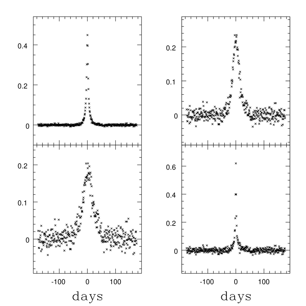
Figure 1: Example of light curves as obtained using the Monte-Carlo simulation procedure described above.

Figure 2: The first 4 principal components corresponding to the simulation presented in Fig. 1.

The functions $\psi(M)$ corresponding to the principal components in the space of the mass function can be computed using Eq. 3. Projecting the data on the principal components is equivalent to projecting the mass function on $\psi(M)$. To illustrate our discussion, an example of $\psi(M)$ functions calculated using the settings of the previous Monte-Carlo simulation are presented in Fig. 3.

Figure 3: The function $\psi(M)$ which corresponds to the principal components. In the right panel we present the 4 original function, while in the other panel we present an orthonormal linear combination of these 4 functions. (Note that in the right panel the function were scaled to have the same amplitude).

3.4 Estimating the mass function.

To illustrate the ability of the method to reconstruct the mass function we will assume that exponent of the mass the mass function, $\alpha$ is unknown. For each simulation we will calculate the 4 principal component of the set of microlensing light curves we have simulated. We will compute the sum of the projection on a principal component of all the light curves $<a_{j}>$. Using Eq. 3 we will calculate the function which corresponds to each principal components in the space of the mass function. Then all we have to do is to compare the projection of a trial mass function with $<a_{j}>$. The trial mass function which match the 4 $<a_{j}>$ as close as possible (in a least-square tens) will be the best mass function. This procedure was applied for 1000 simulation, each time the program derived the best value of the exponent of $\alpha$. The histogram of the values of alpha for the 1000 simulations is presented in Fig. 4.

Figure 4: Histogram of the values of Alpha (the exponent of the mass function) found by fitting the Monte-Carlo simulation by projecting the data in the space of the mass function.

References

- [1] Alard, C., 200, A&AS, in press
- [2] Alard, C., 1999, A&A, 343, 10
- [3] Alard, C., & Lupton, R. 1998, ApJ, 503, 325
- [4] Alard, C., 1997, A&A3, 21, 424
- [5] Alard & Guibert, 1997, A&A, 326, 1
- [6] Alcock et al., 1998, ApJ, 500, 522
- [7] Binney, J., Gerhard, O., Spergel, D., 1997, MNRAS, 288, 365
- [8] Bissantz, N., et al., 1997, MNRAS, 289, 651
- [9] Derue, F. et al., 1999, A&A, 351, 87
- [10] Fux, R., 1997, A&A, 327, 983
- [11] Han, C., 1997, ApJ, 484, 555
- [12] Mao, S., Paczynski, B., 1996, ApJ, 473, 57
- [13] Udalski, A., et al., astro-ph/0002418
- [14] Uglesich, R., et al., 1999, AAS, 194.9004
- [15] Wozniak, P. & Paczyǹski, B., 1997, ApJ, 487, 55
- [16] Zhao, H., 1996, MNRAS, 283, 149
- [17] Zhao, H., Spergel, D.,N., and Rich, R.M., 1995, ApJ, v. 440 L13