Abstract

The spectral energy distribution (SED) of gamma-ray loud BL Lac objects typically has a double-humped appearance usually interpreted in terms of synchrotron self-Compton models. In proton blazar models, the SED is instead explained in terms of acceleration of protons and subsequent cascading. We discuss a variation of the Synchrotron Proton Blazar model, first proposed by Mücke & Protheroe (1999), in which the low energy part of the SED is mainly synchrotron radiation by electrons co-accelerated with protons which produce the high energy part of the SED mainly as proton synchrotron radiation.

As an approximation, we assume non-relativistic shock acceleration which could apply if the bulk of the plasma in the jet frame were non-relativistic. Our results may therefore change if a relativistic equation of state were used. We consider the case where the maximum energy of the accelerated protons is above the threshold for pion photoproduction interactions on the synchrotron photons of the low energy part of the SED. Using a Monte Carlo/numerical technique to simulate the interactions and subsequent cascading of the accelerated protons, we are able to fit the high-energy gamma-ray portion of the observed SED of Markarian 501 during the April 1997 flare. We find that the emerging cascade spectra initiated by gamma-rays from $\pi^{0}$ decay and by $e^{\pm}$ from $\mu^{\pm}$ decay turn out to be relatively featureless. Synchrotron radiation produced by $\mu^{\pm}$ from $\pi^{\pm}$ decay, and even more importantly by protons, and subsequent synchrotron-pair cascading, is able to reproduce well the high energy part of the SED. For this fit we find that synchrotron radiation by protons dominates the TeV emission, pion photoproduction being less important with the consequence that we predict a lower neutrino flux than in other proton blazar models.

ADP-AT-00-1
                                             Astropart. Phys., revised

PACS: 98.70 Rz, 95.30 Gv, 98.54 Cm, 98.58 Fd, 98.70 Sa

Keywords: Active Galaxies: Blazars, BL Lac Objects: individual (Mkn 501),
                  Gamma-rays: theory, Neutrinos, Synchrotron emission, Cascade simulation

1 Introduction

During its giant outburst in April 1997, the nearby BL Lac object Mkn 501 (at redshift z=0.034) emitted photons up to $24$ TeV and $0.5$ MeV in the $\gamma$-ray and X-ray bands, respectively, and has proved to be the most extreme TeV-blazar observed so far (e.g. Catanese et al 1997, Pian et al 1998, Protheroe et al 1998, Quinn et al 1999, Aharonian et al 1999). This energy is the highest so-far observed for any BL Lac object, and the flux is approximately 2 orders of magnitude higher than the synchrotron peak at its quiescent level. BeppoSAX and OSSE observations (Maraschi 1999) suggest that the X-ray spectrum is curved at all epochs, and the spectrum during flaring has been fitted by a multiply-broken power-law (Bednarek & Protheroe 1999). COMPTEL has not seen any significant signal from Mkn 501 at any time (Collmar 1999), while a $3\sigma$ upper limit of $F(>100\,{\rm MeV})<3.6\times 10^{-7}$cm^-2 s^-1 has been derived for the April 1997 EGRET viewing period (Catanese et al 1997).

A flux increase at TeV-energies was also observed with the Whipple, HEGRA and CAT telescopes (Catanese et al 1997), with the most intense flare peaking on April 16 at a level $\sim 100$ times higher than during its quiescent flux. The non-detection of Mkn 501 by EGRET indicates that most of the power output of the high energy component is in the GeV-TeV range. The TeV-observations revealed a power-law spectrum with photon index $\sim 2$ up to $\sim 10$ TeV and a gradual steepening up to 24 TeV. The extragalactic diffuse infrared background leads to significant extinction of $\gamma$-rays through $\gamma\gamma$-pair production above 10 TeV. The extinction-corrected TeV-spectrum (e.g. Bednarek & Protheroe 1999), shows the spectral energy distribution (SED) peaking at $\sim 2$ TeV. Optical observations did not show any significant variations (Buckley & McEnery 1997), indicating that the change in the low energy part of the SED was mainly confined to the X-ray band above $0.1$ keV.

Various models have been proposed to explain the observed $\gamma$-ray emission from TeV-blazars, all of which are identified as high-frequency peaked BL Lac objects. Leptonic models, in which electrons inverse-Compton scatter a population of low energy photons to high energies, currently dominate the thinking of the scientific community. Because of the low luminosity of accretion disks in BL Lacs, the main target photons for the relativistic electrons would be the synchrotron photons produced by the same relativistic electron population, as in the synchrotron self-Compton (SSC) model. An alternative scenario for the production of the observed $\gamma$-ray flux has been proposed involving pion photoproduction by energetic protons with subsequent synchrotron-pair cascades initiated by decay products (photons and $e^{\pm}$) of the mesons (e.g. Mannheim et al 1991, Mannheim 1993). These proton-initiated cascade (PIC) models could, in principle, be distinguished by the observation of high energy neutrinos produced as a result of photoproduction.

In this paper, we consider the April 1997 flare of Mkn 501 in the light of a modified Synchrotron Proton Blazar (SPB) model. We assume that electrons ($e^{-}$) and protons ($p$) are accelerated by 1st order Fermi acceleration at the same shock. The relativistic $e^{-}$ radiate synchrotron photons which serve as the target radiation field for proton-photon interactions, and for the subsequent pair-synchrotron cascade which develops as a result of photon-photon pair production. This cascade redistributes the photon power to lower energies where the photons escape from the emission region, or “blob,” which moves relativistically in a direction closely aligned with our line-of-sight.

Until recently, this model was not able to reproduce the general features of the double-humped blazar spectral energy distribution (SED), but produced a rather featureless spectrum (see e.g. Mannheim 1993), nor could it explain correlated X-ray/TeV-variability. Here, we present a comprehensive description of our Monte-Carlo simulations of a stationary SPB model, including all relevant emission processes, and show that this model is indeed capable of reproducing a double-humped SED as observed. Here, the origin of the TeV-photons are proton synchrotron radiation, as first proposed by Mücke & Protheroe (1999); a similar model has also been proposed by Aharonian (2000), and Rachen (1999) presented speculations about $\mu^{\pm}$- and proton-synchrotron radiation leading to narrow cascade spectra during flares, which might explain correlated X-ray/TeV-variability. Jet energetics and limits from particle shock acceleration, however, put severe constraints on this scenario. The goal of this paper is to discuss the physical processes included in our SPB model Monte-Carlo code, and give the results of applying this code, as an example, to reproduce the SED of the giant flare from Mkn 501 which occurred in April 1997. A comprehensive study of the whole parameter-space (magnetic field, Doppler factor, etc.) for this model will be the subject of a subsequent paper.

In Section 2, we discuss constraints on the maximum particle energies imposed by the co-acceleration scenario, and by the pion production threshold. Section 3 is devoted to the emission processes in the present model. Energy losses and particle production are treated in Sect. 3.1, while the cascade calculations, including a brief description of our code, are outlined in Sect. 3.2. In Sect. 4 we apply our model to the April 1997 flare of Mkn 501. The multifrequency photon spectrum is shown in Sect. 4.1, while in Sect. 4.2 the predicted neutrino spectrum is discussed. We conclude with a discussion and summary in Section 5.

2 The Co-acceleration Scenario

In the present model, shock accelerated protons ($p$) interact in the synchrotron photon field generated by the electrons ($e^{-}$) co-accelerated at the same shock. This scenario may put constraints on the maximum achievable particle energies.

The usual process considered for accelerating charged particles in high energy astrophysics is diffusive shock acceleration (see e.g. Bell 1978, Drury 1983, Blandford & Eichler 1987, Biermann & Strittmatter 1987, Jokipii 1987, Jones & Ellison 1991), in which particles undergo collisionless scattering, e.g. by Alfvén waves, in the upstream and downstream plasma. Charged particles with gyroradii larger than the thickness of the shock front propagate with diffusion coefficients $\kappa_{1}$ and $\kappa_{2}$ in the upstream and downstream plasma, respectively, for propagation parallel to the shock normal. In the shock frame the plasma flow velocity changes from $u_{1}=\beta_{1}c$ in the upstream region to $u_{2}$ in the downstream region. In this paper, for simplicity we restrict ourselves to non-relativistic shocks, and postpone discussion of relativistic shock acceleration to a later paper.

The acceleration time scale for non-relativistic shocks is given by

$$t_{\rm acc}=\frac{3r_{c}\beta}{(r_{c}-1)u_{1}^{2}}(\kappa_{1}+r_{c}\kappa_{2})$$ (1)

where $r_{c}\rightarrow 4$ is the compression ratio for the case of strong shocks in a non-relativistic monoatomic ideal gas. If the magnetic field is governed by an ordered component, the orientation of the shock normal to the main magnetic field direction becomes important. In general, the diffusion coefficient can be written as

$$\kappa_{i}=\kappa_{i,||}\cos^{2}\theta_{i}+\kappa_{i,\perp}\sin^{2}\theta_{i},\hskip 14.22636pti=1,2$$ (2)

where $\theta_{i}$ is the angle between the magnetic field and the axis connecting the upstream ($i=1$) and downstream ($i=2$) regions. In the diffusion limit, kinetic theory relates the parallel and perpendicular diffusion coefficients through

$$\kappa_{||}=[1+\eta^{2}]\kappa_{\perp}=\frac{1}{3}\lambda_{||}\beta c$$ (3)

where $\eta=\lambda_{||}/{r_{g}}$ with $\lambda_{||}$ being the mean free path parallel to the magnetic field, $r_{g}=\beta\gamma mc^{2}/eB$ is the particle’s gyroradius, $m$ and $\gamma=(1-\beta^{2})^{-{1/2}}$ are the particle’s mass and Lorentz factor, respectively, and $B$ is the magnetic field strength in the upstream region. The mean free path is, in general, a function of the particle energy through its gyroradius, and is dependent on the spectrum of the magnetic turbulence. In the small angle scattering approximation (i.e., if Alfvén waves dominate the particle deflection with wavelength equal to the particle gyroradius; see Drury 1983) we have

$$\lambda=\frac{B^{2}r_{g}}{8\pi I(k)k}.$$ (4)

This spectrum $I(k)$ is usually expressed as a power law of the wave number $k$ in the turbulent magnetic field:

$$I(k)\propto k^{-\delta}.$$ (5)

$\delta=5/3$ corresponds to Kolmogorov turbulence which may be common in astrophysical environments (Biermann & Strittmatter 1987), while $\delta=1$ corresponds to Bohm diffusion, and is often considered for simplicity. For strong magnetic fields, Kraichnan turbulence $\delta=3/2$ (Kraichnan 1965) may be present. In the following, we consider $\delta$ as a free parameter. The mean free path may then be expressed as (see Biermann & Strittmatter 1987)

$$\lambda_{||}=\frac{r_{g}}{b(\delta-1)}\left(\frac{r_{g,{\rm max}}}{r_{g}}\right)^{\delta-1}\hskip 8.5359pt\mbox{for}\hskip 8.5359pt\delta\neq 1$$ (6)

$$\lambda_{||}=\frac{r_{g}}{b}\left[\ln\left(\frac{r_{g,{\rm max}}}{r_{g,{\rm min}}}\right)\right]^{-1}\hskip 8.5359pt\mbox{for}\hskip 8.5359pt\delta=1$$

where $b$ is the ratio of the turbulent to ambient magnetic energy density, $r_{g,{\rm max}}$ is the gyroradius of the most energetic protons, and has the same order of magnitude as the system size, and $r_{g,{\rm min}}$ corresponds to the smallest turbulence scale. The mean free path, and consequently the acceleration time at maximum energy is only slightly dependent on the turbulence spectrum in the case of protons, whereas for electrons the acceleration time at maximum energy shows a strong dependence on the magnetic turbulence spectrum adopted.

We expect $b\leq 1$, since otherwise the energy density in particles would not be able to be confined by the ambient field (Biermann & Strittmatter 1987). With these relations, the acceleration time scale may be re-written as

$$t_{\rm acc}=\frac{r_{g}\beta c}{u_{1}^{2}}F(\theta_{1},\eta)$$ (7)

where

$$F(\theta_{1},\eta)=\frac{\eta r_{c}}{r_{c}-1}\left[\cos^{2}{\theta_{1}}+\frac{\sin^{2}{\theta_{1}}}{(1+\eta^{2})}+\frac{r_{c}\cos^{2}{\theta_{1}}+r_{c}^{3}\sin^{2}{\theta_{1}}/(1+\eta^{2})}{(\cos^{2}{\theta_{1}}+r_{c}^{2}\sin^{2}{\theta_{1}})^{3/2}}\right]$$ (8)

The diffusion approximation used here limits the maximum mean free path to $\eta<\beta/\beta_{1}$ (Jokipii 1987). If the particle spectra are cut off due to synchrotron losses, balancing the acceleration time scale with the loss time scale determines the maximum Lorentz factors of protons,

$$\gamma_{p,\rm{max}}=2.1\times 10^{11}\beta_{1}\left[\beta\,B\,F(\theta_{1},\eta_{p,\rm{max}})\right]^{-1/2}$$ (9)

and electrons

$$\gamma_{e,\rm{max}}=1.2\times 10^{8}\beta_{1}\left[\beta\,B\,F(\theta_{1},\eta_{e,\rm{max}})\right]^{-1/2}$$ (10)

where $B$ is in Gauss. The ratio of the maximum proton Lorentz factor to the maximum electron Lorentz factor is then

$$\frac{\gamma_{p,\rm{max}}}{\gamma_{e,\rm{max}}}\leq\frac{m_{p}}{m_{e}}\left[{\frac{F(\theta_{1},\eta_{e,\rm{max}})}{F(\theta_{1},\eta_{p,\rm{max}})}}\right]^{1/2}$$ (11)

where the equality corresponds to the maximum proton energy being determined by synchrotron losses, and the inequality to the maximum proton energy being determined instead by adiabatic losses. For parallel shocks this relation is consistent with the results found by Biermann & Strittmatter (1987).

The corresponding acceleration time scales at the maximum particle energies, if determined by synchrotron losses, are

$$t_{\rm{acc},p,\rm{max}}=2.2\times 10^{7}B^{-3/2}\beta_{1}^{-1}\left[\beta F(\theta_{1},\eta_{p,\rm{max}}\right]^{1/2}\;\;\;\;{\rm s}$$ (12)

for protons, and

$$t_{\rm{acc},e,\rm{max}}=6.6B^{-3/2}\beta_{1}^{-1}\left[\beta F(\theta_{1},\eta_{e,\rm{max}}\right]^{1/2}\;\;\;\;{\rm s}$$ (13)

for electrons. In the present paper, we shall adopt $\beta_{1}=0.5$, $\beta=1$ and $r_{c}=4$. The geometry dependent term $[F(\theta_{1},\eta_{p,\rm{max}})]^{1/2}$ is plotted in Fig. 1a as the dashed curves for different $\eta_{p,\rm{max}}$ values and $r_{c}=4$. It can be seen that highly oblique shocks allow proton acceleration on very short time scales. In the limiting case of a perpendicular shock, drift–shock acceleration drives the energy gain, and the finite size of the shock front restricts the maximum particle energy. The maximum proton Lorentz factor $\gamma_{p}$ is reached for the maximum drift distance, the shock size, and is given by

$$\gamma_{p,\rm{max}}=3.2\times 10^{-7}\beta_{1}RB$$ (14)

with $R$ in cm and $B$ in Gauss.

At their maximum Lorentz factors, the acceleration process for protons is considerably slower than for electrons, and so the proton acceleration time must be consistent with the observed variability time, $t_{\rm var}$,

$$t_{\rm var}D\geq t_{\rm{acc},p,\rm{max}}$$ (15)

where $D$ the Doppler factor. This can be converted to a constraint on the geometry dependent term using Eq. 12, and is plotted as a function of $\theta_{1}$ in Fig. 1a for a typical set of TeV-blazar parameters ($B\approx 20$ G, $D\approx 10$, $t_{\rm var}=12$ hours). The region below the solid line is allowed by the variability constraint (Eq. 15), and gives for each $\eta_{p,\rm{max}}$ value a minimum shock angle between $69^{\circ}$ and $88^{\circ}$, depending on $\eta_{p,\rm{max}}$. Thus, proton shock acceleration on hour time scale in hadronic models can only take place in oblique shocks, and the maximum drift distance may restrict the maximum energy gain rather than the gyroradius.

Using the same shock geometry and magnetic turbulence spectra for both protons and electrons, we find that the ratio $F(\theta_{1},\eta_{e,\rm{max}})/F(\theta_{1},\eta_{p,\rm{max}})$ does not vary by more than a factor of 2 within the allowed shock angle range (see Fig. 1b), allowing us to adopt an average value for this ratio for a given parameter combination. Inserting this ratio into Eq. 11 then restricts the ratio of the allowed maximum particle energies to the range below the solid lines shown in Fig. 2. Points exactly on this line represent models where the particle spectra are limited by synchrotron losses and the acceleration time scale is exactly the variability time scale; points below this line apply if adiabatic losses are dominant for protons or the proton acceleration time scale is shorter than the variability time scale in the jet frame. We note that for a given maximum proton energy, the highest maximum electron energy occurs with Bohm diffusion.

In hadronic blazar models pion photoproduction is essential for neutrino production. The threshold for this process is given by $\epsilon_{\rm{max}}\gamma_{p,\rm{max}}=0.0745$ GeV where $\epsilon_{\rm{max}}$ is the maximum photon energy of the target field, which in the Synchrotron Proton Blazar models is in turn produced by the co-accelerated $e^{-}$. In the $\delta$-function approximation for the synchrotron emission, $\epsilon_{\rm{max}}=(3/8)\gamma_{e,\rm{max}}^{2}(B/B_{\rm{cr}})m_{e}c^{2}$ with $B_{\rm{cr}}=4.414\times 10^{13}$ G. Inserting $\epsilon_{\rm{max}}$ into the threshold condition, we find

$$\gamma_{p,\rm{max}}\geq 1.72\times 10^{16}\left(\frac{B}{\rm{1\;Gauss}}\right)^{-1}\gamma_{e,\rm{max}}^{-2}$$ (16)

and this is shown in Fig. 2 as the dashed lines for various magnetic field strengths. Together with Eq. 11 the allowed range of maximum particle energies is then restricted to the area below the solid lines and above the dashed lines in Fig. 2, as shown for example as the shaded area for $B\approx 20$ G and Kolmogorov turbulence. Inspecting hadronic models as presented in the literature (e.g. Mannheim 1993, Mannheim et al 1996, Rachen 1999), we find that most models which are able to fit the observations lie above the Bohm diffusion line (see Fig. 2), indicating that the turbulence spectrum required in common hadronic blazar jet models is likely to be of Kolmogorov/Kraichnan type. Rachen (1999) speculates that the transition between Kolmogorov and Kraichnan type turbulence could be responsible for the difference between low- and high frequency peaked BL Lacs.

Figure 1: (a) $\sqrt{F(\theta_{1},\eta_{p,\rm{max}})}$ versus shock angle (dashed lines) for different $\eta_{p}$ values (numbers attached to the curves) and $r_{c}=4$. Note that the diffusion approximation limits the mean free path to $\eta<\beta/\beta_{1}$. Region below the solid line satisfies $t_{\rm{var}}D\geq t_{acc,p,\rm{max}}$ for a typical set of TeV-blazar parameters $B\approx 20$ G, $D\approx 10$, $u_{1}=0.5c$, $\beta=1$, $r_{c}=4$, $t_{var}=12$ hours. (b) Ratio $\sqrt{F(\theta_{1},\eta_{e,\rm{max}})/F(\theta_{1},\eta_{p,\rm{max}})}$ versus $\theta_{1}$ for different turbulence spectra.

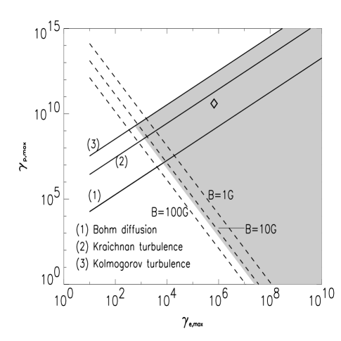
Figure 2: Allowed parameter space (shaded area) for $\gamma_{p,\rm{max}}$, $\gamma_{e,\rm{max}}$ in the SPB-model for different magnetic turbulence spetra. The diamond symbol corresponds to the Mkn 501-model presented below ($B\approx 20$ G, $D\approx 10$, $u_{1}=0.5c$, $\beta=1$, $t_{\rm{var}}=12$ hours).

3 Emission Processes

In the present model, the co-accelerated $e^{-}$ are assumed to produce most of the observed low energy part of the SED by synchrotron radiation, and this is assumed to be the target radiation field for $p\gamma$ interactions and subsequent cascading. The observed hardening of the spectrum with rising flux, has recently been convincingly reproduced by a shock model with escape and synchrotron losses (Kirk et al 1998). The spectral slopes in this model are controlled by synchrotron cooling, and thus naturally explain the temporal behaviour of the spectral index as observed in the X-ray band. The flaring behaviour is explained by the shock front running into plasma whose density is locally enhanced, and which thus increases the number of particles injected into the acceleration process. The increase in the plasma density is accompanied by an increase in the magnetic field, leading to a higher acceleration rate and a shift of the maximum particle energies to higher energies. This picture departs from the standard explanation in which the flat synchrotron spectra appear as a result of a superposition of several local self-absorbed synchrotron spectra with changing self-absorption frequency, adopted in previous PIC models (e.g. Mannheim 1993).

For simplicity, and because we do not wish to include additional parameters, we use the same magnetic field for synchrotron radiation as for acceleration. For normal shocks this approximation is justified as the magnetic fields either side of the shock are similar. This approximation might even be justified for oblique shocks as a lower magnetic field in the upstream region, compared to the downstream region, implies a higher diffusion coefficient and time spent upstream, increasing the synchrotron losses there and partially compensating for having a lower field upstream. Also, at oblique shocks, reflection at the shock front itself is thought to be more important than diffusion in the downstream region (Kirk & Heavens 1989), so that accelerating particles spend most of their time upstream. In addition, we assume that pitch-angle scattering maintains quasi-isotropic particle distributions, and all radiating particles are confined to the homogeneous emission region.

3.1 Energy Losses

There are several energy loss/interaction processes which are important for protons, electrons and photons in a dense radiation field produced by relativistic electrons co-accelerated along with the protons: protons interact with photons, resulting in pion production and (Bethe-Heitler) pair production; electrons, muons, protons and charged pions emit synchrotron radiation; photons interact with photons by pair production. We shall show below that, for the present model, Inverse Compton emission by the electrons can be neglected.

For simplicity we represent the observed synchrotron spectrum of Mrk 501 during flaring, the target photon field for the $p\gamma$-collisions and photon-photon pair production, as a broken power-law:

$$n(\epsilon)\propto\left\{\begin{array}[]{ll}\epsilon^{-1.6}&\mbox{for}\qquad 10^{-7}\rm{eV}\leq\epsilon\leq 1.6~{}\rm{keV}\\ \epsilon^{-1.8\phantom{/2}}&\mbox{for}\qquad 1.6~{}\rm{keV}\leq\epsilon\leq 42~{}\rm{keV}\end{array}\right.$$

For determining the photon density of the target field, the dimension of the emission region, assumed to be spherical, must be known. This can be estimated by setting the photon crossing time equal to the variability time scale (in the jet frame – in the remainder of this section all quantities are in the jet frame unless noted otherwise), making the implicit assumption that the light crossing time scale determines the flux variations. The observed variability time scale can, in general, depend on: (i) the injection time scale for the energetic particles $t_{\rm{acc}}(E)$; (ii) the time needed for converting their energy into radiation, i.e. their energy loss time scale $t_{\rm{loss}}(E)$; (iii) the effective light crossing time $t_{\rm{cross}}(E)\approx(2R_{\rm{blob}}/c)\times P_{\rm{esc}}(E)$ where $R_{\rm{blob}}$ is the geometrical blob radius and $P_{\rm{esc}}(E)$ is the energy dependent probability for photons escaping from the blob taking account of $\gamma\gamma$-pair production and diffusion during cascading. Hence,

$$Dt_{\rm{var}}\approx\max(t_{\rm acc},t_{\rm{loss}},t_{\rm{cross}}).$$ (17)

For leptonic models, the time scales for energy losses and acceleration are typically significantly shorter than the crossing time, i.e. $t_{\rm{loss}}$,$t_{\rm acc}\ll t_{\rm{cross}}$, and thus the radius of the emission region can be derived from the observed variability time scale. In addition, the emission region is assumed to be optically thin at 1 TeV and X-ray energies, implying that $R_{\rm{TeV}}\approx R_{\rm{X}}$, where $R_{\rm{TeV}}$, $R_{\rm{X}}$ are the dimensions of the emitting region at 1 TeV and X-ray energies, respectively. This differs in two points from the hadronic blazar jet models: Firstly, the optical depth of the emission region is strongly energy dependent, leading to an effective, i.e. observed, thickness of the emission region $R_{\rm{eff}}(E)\approx R_{\rm{blob}}P_{\rm{esc}}(E)$, which also depends on the energy. Diffusion can be neglected during cascading since the cascade processes are of leptonic origin, and are, in general, more rapid than diffusion. Thus, in SPB models the crossing time scale in the optically thick TeV-band is related to the crossing time scale at X-ray energies (optically thin), through

$$t_{\rm{cross,TeV}}\approx t_{\rm{cross,X}}[1-\exp(-\tau_{\gamma\gamma,\rm{TeV}})]/\tau_{\gamma\gamma,\rm{TeV}}$$ (18)

(averaging over a homogeneous emission volume; see Rachen 1999). Hence, $t_{\rm{cross,X}}$ is the relevant time scale for estimating the radius $R_{\rm{blob}}\approx R_{X}$ of the emission region. Secondly, the acceleration and/or energy loss time scales can be of the same order of magnitude as the crossing time scale. Acceleration, however, is always faster than the energy losses of the accelerating particles up to their maximum energy. Note that because of the leptonic nature of the cascade processes, the energy loss time scale will in general be determined by the (slower) hadronic processes. As a further consequence, flux variations are not significantly washed out by the cascading mechanism, but closely follow the crossing or hadronic loss time scales.

If $t_{\rm{loss}}\leq t_{\rm{cross}}$ the crossing time scale determines the flux variations, and in this case we can estimate the radius of the emission region through $R_{\rm{blob}}\approx 0.5cDt_{\rm{var,X}}$ with $t_{\rm{var,TeV}}\approx t_{\rm{var,X}}/\tau_{\gamma\gamma,\rm{TeV}}$. In our present model, efficient proton synchrotron emission determines the TeV-bump in the blazar SED, and so at the maximum proton energy $t_{\rm{ad}}>t_{p,\rm{syn}}$. The adiabatic loss time scale due to expansion is (Longair 1994)

$$t_{\rm{ad}}=R_{\rm{ad}}^{-1}\equiv|R_{\rm{blob}}/\dot{R}_{\rm{blob}}|=2|B/\dot{B}|\approx R/u_{1}$$ (19)

assuming magnetic flux conservation $B\propto R_{\rm{blob}}^{-2}$, and so $t_{\rm{ad}}$ is related to the size of the emission region $R_{\rm{blob}}$. Since $t_{\rm{loss}}\approx t_{p,\rm{syn}}$ for the highest proton energies in our model responsible for the TeV-emission, $t_{\rm{loss}}\leq t_{\rm{cross}}$, and so the size of the emission region can be determined by the variability time scale.

The shortest doubling time measured by the Whipple Telescope in the 1997 data of Mkn 501 was approximately 2 hours (Quinn et al 1999), while HEGRA reported a lower doubling time of 15 hours (Aharonian et al 1999) or 12 hours (Krawczynski 1999). As a working hypothesis we adopt here a variability time scale of 12 hours, but will discuss also effects of smaller variability time scales. For $t_{\rm{var}}\approx 12$ hours we find $R_{\rm{blob}}\approx 8\times 10^{15}$cm for $D\approx 10$.

Eq. 12 and 13 imply that the acceleration time scale for electrons is much smaller than for protons at their maximum energies, $t_{acc,e,\rm{max}}\ll t_{acc,p,\rm{max}}$. If a $\gamma$-ray outburst thus corresponds to particle acceleration of a single $p/e^{-}$ population, then an increase of the low energy synchrotron flux will occur before the TeV-flare. The amount of the lag depends on the proton acceleration time, and so on the shock parameters, in particular the diffusion coefficients. E.g. for the present model and the Kolmogorov spectrum $t_{acc,p,\rm{max}}\approx 10^{5}$ s (see Fig. 3), which for D=10 suggests a time lag of $\approx 5$ hours. For Bohm diffusion, the time lag would be $\approx 14$ hours. These time lags are consistent with current observational constraints.

The relevant radiation and loss time scales for photomeson production, Bethe-Heitler pair production, $p$ synchrotron radiation, and adiabatic losses due to jet expansion, are shown in Fig. 3 together with the acceleration time scale. Synchrotron losses, which turn out to be at least as important as losses due to photopion production in our model, limit the injected $p$ spectrum to a Lorentz factor of $\gamma_{p}\approx 3\times 10^{10}$ for the assumed model parameters. We adopt a Kolmogorov spectrum of turbulence for the magnetic field structure ($\delta=5/3$), and so for any $\eta_{p}\geq 1$ value, variability arguments constrain the shock angle to $\theta_{1}\geq 75^{\circ}$ (see Fig. 1). The maximum proton energy could then be achieved, e.g., with $\eta_{p}=10$, $\theta_{1}=85^{\circ}$ and $u_{1}=0.5c$. This is in agreement with the limit imposed on quasi-perpendicular shocks due to their finite shock size. Note that due to the non-zero shock angle, the acceleration time scale shown in Fig. 3 does not follow a strict power-law, but is curved. This is due to the non-linear dependence of $F(\theta_{1},\eta_{p})$ on the particle’s gyroradius (see Eqs. 6–8). A $\gamma_{p}^{-2}$ proton spectrum, typical of shock accelerated particles, is used for $2\leq\gamma_{p}\leq\gamma_{p,{\rm max}}$, where $\gamma_{p,{\rm max}}=3\times 10^{10}$ is obtained from requiring $t_{{\rm acc,}p}=t_{{\rm syn,}p}$ at $\gamma_{p,{\rm max}}$.

Rachen & Mészáros (1998) noted the importance of synchrotron losses of $\mu^{\pm}$ (and $\pi^{\pm}$) prior to their decay in AGN jets and GRBs. The critical Lorentz factors $\gamma_{\mu}\approx 2\times 10^{9}$ and $\gamma_{\pi}\approx 4\times 10^{10}$, above which synchrotron losses in the assumed magnetic field dominate over decay, lie below the maximum Lorentz factor for $\mu^{\pm}$ and above the maximum Lorentz factor for $\pi^{\pm}$. Thus, while $\pi^{\pm}$-synchrotron losses can safely be ignored, $\mu^{\pm}$-synchrotron losses should be included.

For the parameters employed in this work we receive a target photon energy density of $u_{\rm{target}}\approx 0.06~{}\rm{TeV/cm}^{3}$, and a magnetic field energy density of $u_{B}\approx 11.7~{}\rm{TeV/cm}^{3}$ using $B\approx 20$ G. With $u_{B}\gg u_{\rm{target}}$ significant Inverse Compton radiation from the co-accelerated $e^{-}$ is not expected.

We also neglect secondary production interactions of relativistic protons with the ambient thermal plasma. In the present model the dominant loss process turns out to be proton synchrotron radiation. Thus, our assumption is justified if the thermal proton density does not exceed $\approx 10^{9\ldots 10}$ cm^-3. In Section 4 we estimate the number density of cold protons to be less than this for reasonable values of the jet width.

Figure 3: Mean energy loss time of $p$ for $\pi$-photoproduction ($\pi$), Bethe-Heitler pair production ($e^{+}e^{-}$) and synchrotron radiation (syn). Loss times for $\pi^{\pm}$- and $\mu^{\pm}$ for synchrotron radiation (syn $\pi$, syn $\mu$) are also shown and compared with their mean decay time scales (decay $\pi$, decay $\mu$). The acceleration time scale (acc), based on Kolmogorov turbulence, is calculated for $r_{c}=4$, $u_{1}=0.5c$ and shock angle $\theta_{1}=85^{\circ}$. The curvature of the acceleration time scale is caused by the non-linear dependence of $F(\theta,\eta_{p})$ on $\gamma$. The adiabatic loss time (adiab) is assumed to be $2|B/\dot{B}|\approx R/u_{1}\approx Dt_{\rm{var}}$. We adopt $B\approx 20$ G, and all quantities are in the co-moving frame of the jet.

3.2 Simulation of particle production and cascade development

For the first time in the context of the SPB-model, we use the Monte-Carlo technique to simulate particle production and cascade development, and this allows us to use exact cross sections. For photomeson production we use the Monte-Carlo code SOPHIA (Mücke et al 2000), and Bethe-Heitler pair production is simulated using the code of Protheroe & Johnson (1996). We calculate the yields for both processes separately, and the results are then combined according to their relative interaction rates.

The mean pion production interaction rate for an isotropic photon field is

$$r_{\pi}(E_{p})=\frac{1}{8E_{p}^{2}\beta_{p}}\int_{\epsilon_{\rm th}}^{\infty}\!d\epsilon\,\frac{n(\epsilon)}{\epsilon^{2}}\int_{s_{p,\rm th}}^{s_{p,\rm max}}\!ds_{p}\,(s_{p}-m_{p}^{2})\sigma_{\pi}(s_{p})\ ,$$ (20)

where $s_{p}=m_{p}^{2}+2E_{p}\epsilon(1-\beta_{p}\cos\theta_{p})$ is the center-of-momentum (CM) energy squared, $\theta_{p}$ the angle between the proton and the photon, $\beta_{p}c$ the proton’s velocity, $\sqrt{s_{p,\rm th}}\approx 1.08$GeV the threshold CM energy, $\epsilon_{\rm th}=(s_{p,\rm{th}}-m_{p}^{2})/2(E_{p}+p_{p})$, $s_{p,\rm max}=m_{p}^{2}+2E_{p}\epsilon(1+\beta_{p})$ and $\sigma_{\pi}$ the pion production cross section. The Bethe-Heitler pair production interaction rate, $R_{\rm{BH}}$, is calculated using the formulae given in Chodorowski (1992).

In highly magnetized environments, proton-photon interactions compete with synchrotron radiation by the protons. To take proton synchrotron losses into account in our code, we sample a $p\gamma$ interaction length from an exponential distribution with its corresponding mean $\bar{x}_{p\gamma}=c/r_{\pi,BH}$ as given below. We make the approximation that the proton energy on interacting is given by

$$E_{p}\approx E_{p}^{(0)}\left[1+{x_{p\gamma}\over\bar{x}_{p,syn}(E_{p}^{(0)})}\right]^{-1}$$ (21)

where $E^{(0)}_{p}$ is the initial proton energy, $x_{p\gamma}$ is the sampled interaction length for pion production or Bethe-Heitler pair production, and $\bar{x}_{p,\rm{syn}}=c/r_{p,\rm{syn}}$ is the proton synchrotron loss distance given by

$$r_{M,\rm{syn}}=\frac{4}{3}\left(\frac{m_{e}}{M}\right)^{2}{\sigma_{T}\gamma u_{B}\over Mc}.$$ (22)

where $M=m_{p}$, $\sigma_{T}$ is the Thomson cross section, and $u_{B}$ is the magnetic energy density.

The relatively long mean life time of highly energetic charged pions, muons and kaons might be of the same order of magnitude as their synchrotron loss time scale in highly magnetized environments like AGN jets and GRBs (Rachen & Mészáros 1998). We simulate their synchrotron energy losses by sampling the decay length $x_{\rm{dec}}$ from an exponential distribution with corresponding mean decay length $\bar{x}_{\rm{dec}}=c\gamma\tau_{\rm{dec}}$. For $\mu^{\pm}$ we have $\tau_{\rm{dec}}=2.20\times 10^{-6}$ s, while $\tau_{\rm{dec}}=2.60\times 10^{-8}$ s for $\pi^{\pm}$ and $\tau_{\rm{dec}}=1.24\times 10^{-8}$ s for $K^{\pm}$. The particle’s energy on decaying is then

$$E_{K,\pi,\mu}=E^{(0)}_{K,\pi,\mu}\left[1+{2x_{dec}\over\bar{x}_{K,\pi,\mu,\rm{syn}}(E^{(0)}_{K,\pi,\mu})}\right]^{-1/2}.$$ (23)

where $E^{(0)}_{K,\pi,\mu}$ is the initial $K$,$\pi$, or $\mu$ energy, $\bar{x}_{K,\pi,\mu,\rm{syn}}=c/r_{K,\pi,\mu,\rm{syn}}$ is the synchrotron loss distance with $r_{K,\pi,\mu,\rm{syn}}$ given by Eq. 22 for $M=m_{K}$, $m_{\pi}$ or $m_{\mu}$.

We next outline the simulations of the cascade development in more detail. Energetic photons will pair produce on the target photon field, and if the magnetic energy density exceeds the injected target field density ($u_{\rm{B}}>u_{\rm{target}}$) they will initiate a pair-synchrotron cascade. Energetic photons arise directly from $\pi^{0}$-decay, or indirectly as synchrotron photons from protons, charged mesons and electrons resulting from $\pi^{\pm}\rightarrow\mu^{\pm}\rightarrow e^{\pm}$ decay and Bethe-Heitler pair production. The optical depth $\tau_{\gamma\gamma}(E_{\gamma})$ for $\gamma$-ray photons with energy $E_{\gamma}$ for $e^{\pm}$ pair production inside the blob is given by

$$\tau_{\gamma\gamma}(E_{\gamma})=\frac{R_{\rm{blob}}}{8E^{2}_{\gamma}}\int_{\epsilon_{\rm{min}}}^{\infty}d\epsilon\frac{n(\epsilon)}{\epsilon^{2}}\int_{s_{\gamma,\rm{min}}}^{s_{\gamma,\rm{max}}(\epsilon,E_{\gamma})}ds_{\gamma}s_{\gamma}\sigma_{\gamma\gamma}(s_{\gamma})$$ (24)

where $n(\epsilon)$ is the differential photon number density and $\sigma_{\gamma\gamma}(s)$ is the total cross section for photon-photon pair production (Jauch & Rohrlich 1955) for a centre of momentum frame energy squared given by

$$s_{\gamma}=2\epsilon E_{\gamma}(1-\cos{\theta_{\gamma}})$$ (25)

where $\theta_{\gamma}$ is the angle between directions of the energetic photon and soft photon, and $s_{\gamma,\rm{min}}=(2m_{e}c^{2})^{2}$, $s_{\gamma,\rm{max}}=4\epsilon E_{\gamma}$ and $\epsilon_{\rm{min}}=(m_{e}c^{2})^{2}/E_{\gamma}$. For simulating photon-photon pair production we approximate $E_{e^{+}}=E_{e^{-}}=E_{\gamma}/2$. The radiating $e^{\pm}$ are assumed to be continuously isotropized in the blob frame by deflection in the uniform magnetic field, resulting in the synchrotron radiation being isotropic in the blob frame. The spectrum of synchrotron photons, averaged over pitch-angle because of the isotropy of the particle distribution, is calculated using functions given by Protheroe (1990).

In general, the cascade can be initiated by photons from $\pi^{0}$-decay (“$\pi^{0}$ cascade”), electrons from the $\pi^{\pm}\to\mu^{\pm}\to e^{\pm}$ decay (“$\pi^{\pm}$ cascade”), $e^{\pm}$ from the proton-photon Bethe-Heitler pair production (“Bethe-Heitler cascade”) and $p$ and $\mu$-synchrotron photons (“$p$-synchrotron cascade” and “$\mu^{\pm}$-synchrotron cascade”). Here, we assume the cascades develop linearly, and this requires the photon field produced by the cascade, to be negligible as a target field in comparison with the injected synchrotron radiation due to co-accelerated $e^{-}$. This requirement can be expressed as $\tau_{\gamma\gamma,\rm{cas}}\ll\tau_{\gamma\gamma,\rm{target}}$ with $\tau_{\gamma\gamma,\rm{target}}$,$\tau_{\gamma\gamma,\rm{cas}}$ being the pair production optical depths of photons on the target and cascade photon field, respectively. Our Monte-Carlo results show this condition to be met for the present input. To simplify the calculation, the electrons are completely cooled instantly by synchrotron radiation before pair production by the synchrotron photons takes place. This approximation is equivalent to assuming that $t_{\rm{syn}}\ll t_{\rm{pair}}$ which is justified because of the very short synchrotron life time of electrons in the assumed magnetic field.

A matrix method (e.g. Johnson et al 1996) is then used to follow the pair-synchrotron cascade in the ambient synchrotron radiation field and magnetic field. The cascades are considered in the jet frame. Here, electron and photon fluxes are represented by vectors $G_{j}^{k}$ and $F_{i}^{k}$, which give the total number of electrons in the energy bin at energy $E_{j}$ and number of photons at energy $E_{i}$, respectively, in the $k$th cascade generation. We use a logarithmic stepsize of 0.1 ranging from $\log({E_{e}/1\,\rm{GeV}})=-3$ to $12$ in electron energy, and from $\log({E_{\gamma}/1\,\rm{GeV}})=-13$ to $12$ in photon energy. Averaged over a homogeneous emission region, the probability of gamma-ray interaction by photon-photon pair production at energy $E_{i}$ is given by the vector $P_{\rm{\gamma\gamma},i}$

$$P_{\rm{\gamma\gamma},i}=[1-P_{\rm{esc}}(E_{i})]=\left[1-\frac{1-\exp(-\tau_{\gamma\gamma}(E_{i}))}{\tau_{\gamma\gamma}(E_{i})}\right].$$ (26)

The transfer matrix $T^{(\rm{syn})}_{ij}$ gives the number of synchrotron photons of energy $E_{i}$ produced by electrons of energy $E_{j}$, $T^{(\rm{syn})}_{ij}$, and the transfer matrix $T^{(\rm{pair})}_{ij}$ gives the number of $e^{\pm}$ of energy $E_{j}$ produced through pair production of energetic photons of energy $E_{i}$ on the target field. The vectors and matrices are calculated taking care of energy conservation.

The photon and electron fluxes due to synchrotron radiation and photon-photon pair production are then calculated through matrix multiplication. We start by calculating the number of $\pi^{0}$-decay photons which pair produce in the blob

$$F_{i}^{0}=I_{i}^{0}P_{\rm{\gamma\gamma},i}$$

where the vector $I_{i}^{0}$ gives the number of $\pi^{0}$-decay gamma-rays at an energy $E_{i}$ (the emerging photons, i.e. those which do not pair produce in the blob, are stored in an array). The electron spectrum due to photon-photon pair production is then given by

$$F_{j}^{1}=\sum_{i}F_{i}^{0}T^{(\rm{pair})}_{ij}.$$

These electrons radiate synchrotron photons, and the resulting photon yield is determined by

$$I_{i}^{1}=\sum_{j}F_{j}^{1}T^{(\rm{syn})}_{ij}.$$

This is the 1st cascade generation photon spectrum, which in turn again suffers photon-photon pair production on the target photon field in the blob, etc. In our calculation, we iterate until $F_{i}^{k}\leq 0.01$ at any energy $E_{i}$, or stop at 10 generations.

We have injected $10^{4}$ protons at each proton energy equally spaced in $\log E_{p}$ at 0.1 decade intervals from $10^{3}$ GeV to the maximum injection energy. These protons are assumed to be continuously isotropized, and interact with the synchrotron radiation field of the co-accelerated $e^{-}$ through pion production and Bethe-Heitler pair production. The resulting neutrinos (see Sect. 4.1) escape without further interaction, but the $e^{\pm}$ and high energy $\gamma$-rays initiate cascades. The resulting particle spectra were weighted with $n_{p,0}E_{p}^{-2}dE_{p}$, appropriate to the assumed proton injection spectrum, and divided by the number of injected protons, and by $4\pi$ steradians. Figs. 4 and 5 show examples of cascade spectra in the observer’s frame initiated by photons with different origins for model parameters (given above), which satisfactorily reproduce the flare spectrum of Mkn 501.

Our Monte-Carlo program only treats the first interactions of protons, and so we must take account of this when making the final flux predictions. In the case of pion production, a fraction $\kappa\approx 0.25$ of the initial proton energy goes into particle production, and $\sim 1/3$ of the time the emerging nucleon is a neutron, and is assumed to escape from the blob without further interaction. Combining these two factors, the resulting spectra must be multiplied by 2.01 to take account of subsequent pion production interactions. Similarly, the multiplication factor which takes account of subsequent Bethe-Heitler pair production interactions is $\sim 10$. Particle spectra due to pion production and Bethe-Heitler pair production are then weighted according to their mean interaction rates, i.e. $R_{\pi}/R_{\rm{tot}}$ for pion production, and $R_{\rm{BH}}/R_{\rm{tot}}$ for Bethe-Heitler pair production where $R_{\rm{tot}}=R_{\pi}+R_{\rm{BH}}+R_{\rm{ad}}$ is the total interaction rate, taking into account adiabatic losses of the protons due to jet expansion approximated by Eq. 18.

Adiabatic jet expansion also affects the radius of the emission region, its photon density and magnetic field, and thereby the probability for $p\gamma$-interactions and the subsequent cascade development. With the expansion of the emission region, the probability for $p\gamma$-interactions decreases because of the decrease of the photon energy density and magnetic field. It follows that $p\gamma$-interactions, and their resulting cascades, most likely take place during the initial phase of the jet expansion, and so we neglect any effects on the emerging cascade spectra due to changes in magnetic field or dimension of the emission region. In particular, the flare rise-time can be much shorter than the expansion and light crossing time scales if one associates it with the onset of the $p\gamma$-interactions and their resulting cascades. Short rise-times and longer flare decay time scales are typically observed in blazar light curves. Finally, we transform the cascade spectrum to the observer’s frame. For calculating the distance, $q_{0}=0.5$ and $H_{0}=50$ km s^-1 Mpc^-1 are used.

Cascades initiated by photons from $\pi^{0}$ decay, “$\pi^{0}$ cascades”, or by electrons from $\pi\to\mu\to e$ decay, “$\pi^{\pm}$ cascades”, (Fig. 4) produce rather featureless spectra (see also Mannheim et al 1993). However, cascades initiated by protons “$p$-synchrotron cascades”, and by muons from $\pi\to\mu\to e$ decay, “$\mu^{\pm}$-synchrotron cascades” (Fig. 5b) produce a double-humped SED as observed for $\gamma$-ray blazars (see also Rachen 1999). The contribution from Bethe-Heitler pair production turns out to be negligible (Fig. 5a). In the model for Mkn 501 presented here, the synchrotron flux from directly accelerated $e^{-}$ significantly exceeds the reprocessed $\mu$ and $p$ synchrotron flux. Thus, in the present Mkn 501 model direct proton and muon synchrotron radiation is mainly responsible for the high energy hump whereas the low energy hump is mainly synchrotron radiation by the directly accelerated $e^{-}$. In the present model photons up to 1 TeV in the jet frame are optically thin to $\gamma\gamma$-pair production. Thus, only a small fraction of the power emitted as proton synchrotron radiation is redistributed to lower energies via cascading. For models where the optical depth of TeV-photons is significantly higher, a correspondingly larger fraction of the TeV-bump may be redistributed to X-ray energies. In these models, the pairs produced by photons of the “high energy hump” may contribute considerably to the observed X-ray bump, whereas in the present model they are negligible in comparison to the directly accelerated electrons. We note that for the case of strong magnetic fields where $\mu^{\pm}$-synchrotron cascades cause detectable humps, the $p$ cascade spectrum dominates in general over the $\mu^{\pm}$ cascade spectrum.

Figure 4: (a) Average cascade spectrum initiated by $\pi^{0}$-decay, and (b) $\pi^{\pm}\rightarrow\mu^{\pm}\rightarrow e^{\pm}$-decay synchrotron photons (lower panel). Dot-dashed and dotted histogram shows the 1st and 2nd generation synchrotron photons on production. Solid histogram shows the emerging photon spectrum on production.

Figure 5: (a) Average emerging cascade spectrum initiated by Bethe-Heitler pair production. (b) Average emerging cascade spectrum initiated by $p$- (solid histogram) and $\mu^{\pm}$-synchrotron photons (dot-dashed histogram). Note the different vertical scale in both figures.

4 Application to the April 1997 flare of Mkn 501

Adding the four components of the cascade spectra in Fig. 4-5 we obtain the SED shown in Fig. 6 where it is compared with the multifrequency observations of the 16 April 1997 flare of Mkn 501. We use the parametrization of Bednarek & Protheroe (1999) to represent the BeppoSAX+OSSE data (thick straight line at low energies). The broken power-law simplification (Eq. 3.1) used as the target radiation field for $p\gamma$-interactions and $\gamma\gamma$ interactions is shown by the chain line. The 100 MeV upper limit from Catanese et al (1997) is nearly simultaneous to the TeV-flare observations. The TeV-flux, corrected for pair production on the cosmic background radiation field (Bednarek & Protheroe 1999) for two different background models, is shown as the thick curves.

The parameters used for modeling the April 1997 flare are: $D=12$, $B\approx 20$ G, radius of the emission region $R_{\rm{blob}}=8\times 10^{15}$ cm. For a target photon field for the $p\gamma$-interactions, and the cascades as given in Eq. 16, we find a photon energy density of this radiation field of $u_{\rm{target}}=60$ GeV/cm^-3. The accelerated protons are assumed to follow a power law $\propto\gamma_{p}^{-2}$ between $2\leq\gamma_{p}\leq\gamma_{p,\rm{max}}=3\times 10^{10}$, and in order to fit the emerging cascade spectra to the data a proton number density of $n_{p}\approx 250$ cm^-3, corresponding to an energy density of accelerated protons of $u_{p}\approx 11.6$ TeV/cm^-3 is required. With a magnetic field energy density of $u_{B}\approx 11.7$ TeV/cm^-3 our model satisfies $u_{\rm{target}}\leq u_{p}\approx u_{B}$ (all parameters are in the co-moving frame of the jet), confirming that a significant contribution from inverse-Compton scattering is not expected.

To calculate the total jet luminosity $L_{\rm{jet}}$, measured in the rest frame of the galaxy, we adapt the formulae of Bicknell (1994) and Bicknell & Dopita (1997) given for the synchrotron self-Compton model to apply for the case of our proton blazar model. We receive

$$L_{\rm jet} = {L^{\rm high}_{\rm obs}\over D^{2}\zeta_{p}}\left[\chi_{p}{(\Gamma-1)\over\Gamma}+1+{p_{B}\over p_{p}}+{\zeta_{p}S^{\rm low}_{\rm obs}\over\zeta_{e}S^{\rm high}_{\rm obs}}\right]$$ (27)

where $\Gamma=(1-\beta^{2})^{-1}\approx D/2$ is a good approximation to the Lorentz factor of jets closely aligned to the line of sight, and the four terms inside the bracket give the relative contributions to the total jet power of cold protons, accelerated protons, magnetic field, and accelerated electrons, respectively. The contribution from cold protons is estimated on the basis of charge neutrality. $S^{\rm low}_{\rm obs}$ and $S^{\rm high}_{\rm obs}$ are the observed bolometric fluxes of the low and high energy component, respectively, and $\zeta_{e}\approx 1$, $\zeta_{p}$ are the radiative efficiencies for electrons and protons. $L^{\rm high}_{\rm obs}=4\pi d^{2}S^{\rm high}_{\rm obs}$ with $d$ the luminosity distance, $p_{B}=[B^{2}/(2\mu_{0})]/3$ and

$$p_{p}={L^{\rm high}_{\rm obs}\over 4D^{2}\zeta_{p}\Gamma^{2}\beta c\pi R_{blob}^{2}}$$ (28)

gives the jet-frame pressure of relativistic protons that would apply in the absense of energy loss mechanisms, and

$$\chi_{p}={3\over 4}\left({m_{p}\over m_{e}}{\zeta_{p}S^{\rm low}_{\rm obs}\over\zeta_{e}S^{\rm high}_{\rm obs}}{1\over{\gamma_{e}}_{1}\ln({\gamma_{e}}_{2}/{\gamma_{e}}_{1})}-{1\over{\gamma_{p}}_{1}\ln({\gamma_{p}}_{2}/{\gamma_{p}}_{1})}\right).$$ (29)

We use this formula to estimate the total jet power to be $\approx 10^{46}$ erg/s, and we find the contributions to the total jet power of cold protons, magnetic field, and accelerated electrons, relative to that of accelerated protons, to be 0.8, 1, and 0.01, respectively, with a number density of cold protons $\approx 10^{4}$ cm^-3. Thus, for the shock acceleration mechanism we require more power per particle going into relativistic protons than into electrons.

Fig. 7 shows the dependence of the total jet luminosity on the Doppler factor $D$ with fixed parameters $t_{\rm{var}}=12$ hours, $\beta_{1}=0.5$, and with $B$, $R$, $n_{p}$ and $u_{\rm target}$ being of Mkn 501 during flaring. Clearly visible is the fact that in hadronic models the proton kinetic energy and the poynting flux dominate the total jet luminosity, while the electron kinetic energy is only of minor importance. At high Doppler factors the emission region becomes so large that one needs only relatively small magnetic fields and proton densities to fit the observations. In addition, adiabatic losses become small resulting in a decrease of the required kinetic proton luminosity. For example, $B\approx 5$ G and $n_{p}\approx 10^{-2}$ cm^-3 are sufficient to fit the Mkn 501 flare for $D=50$, while for $D=8$ magnetic fields of over 30 G and proton densities of $n_{p}\approx 10^{4}$ cm^-3 are needed. The total jet luminosity exhibits a minimum of $\approx 10^{46}$erg/s at around $D\approx 12$, which corresponds to the model we have chosen to present here.

Smaller variability time scales in the shock acceleration model can only be explained by quasi-perpendicular shocks with a large mean free path (see Fig. 1a), which in turn are only consistent with the diffusion approximation for low shock speeds. Due to the size limit of the shock, the maximum energy gain is then limited to significantly lower values, and one may not reach TeV-photon energies in the proton synchrotron model, unless the magnetic field is increased accordingly, which in turn leads to larger jet luminosities. For example, for $D=10$ and a variability time scale of 12 hours, at least B=20 G is needed to comply with all acceleration constraints. For $t_{\rm{var}}=3$ hours, one needs at least 50 G. In comparison, leptonic models would give a minimum jet luminosity of $\approx 10^{44}$ erg/s for this flare (Ghisellini 1998), about two orders of magnitude lower. This is due to the much lower magnetic fields invoked there, and the less massive particles which drive the kinetic flow.

In the framework of the jet–disk symbiosis (e.g. Falcke & Biermann 1995), the jet luminosity should not exceed the total accretion power $Q_{\rm{accr}}$ for the equilibrium state. Accretion theory relates the disk luminosity to the accretion power. Page & Thorne (1974) give $L_{\rm{disk}}\approx(0.05-0.3)Q_{\rm{accr}}$. Disk luminosities for ’typical’ radio-loud AGN lie in the range $L_{\rm{disk}}\approx 10^{44}-10^{48}$ erg/s with BL Lac objects tending to the lower end on average. Specifically, for Mkn 501 there are no emission line measurements available, and this complicates the evaluation of the disk luminosity for this object. However, any observed UV-emission in the flaring stage may put an upper limit on it. Again only historical data are available here, leaving room for speculation. We estimate $L_{\rm{disk}}\approx 10^{43}-10^{44}$ erg/s (Mufson et al 1984, Pian et al 1998), and obtain for the accretion power, $Q_{\rm{accr}}\approx(3-200)\cdot 10^{43}$ erg/s, at least a factor 5 below the necessary value to comply with the constraint of the disk–jet symbiosis. Note, however, that the estimate of $Q_{\rm{accr}}$ is based on archival non-flaring data from Mkn 501, and we could speculate that either the disk has pushed more energy into the jet during TeV-flaring, or that the flaring stage can not be considered as a steady state. Also, accretion theory might predict larger conversion efficiencies of the accretion power into disk radiation than actually might occur in BL Lac objects.

It is also instructive to consider the radiative efficiency of the proposed model in comparison to alternative models. Using Eq. 29 we estimate the radiation efficiency of the protons we find $\zeta_{p}\approx 0.01$. This is similar to the value of $\zeta_{p}$ in the Proton-Blazar model proposed by Mannheim (1993), and is fully in agreement with the results presented by Celotti & Fabian (1993) on a basis of a sample of 105 sources. In comparison, leptonic models would give two orders of magnitude higher radiation efficiencies.

Figure 6: Best-fit model (histogram) in comparison with the data of the 16 April 1997-flare of Mkn 501. Photon absorption on the cosmic diffuse background radiation field is not included. Straight solid lines: parametrization of the observed synchrotron spectrum (BeppoSAX & OSSE) and observed TeV-emission corrected for cosmic background absorption (Bednarek & Protheroe 1999); the 100 MeV upper limit is from Catanese et al 1997 (observed 9-15 April 1997); dashed-dotted line: input target spectrum.

Figure 7: Dependence of total jet luminosity $L_{\rm{jet}}=L_{B}+L_{\rm{p,hot}}+L_{\rm{p,cold}}+L_{\rm{e}}$ and its different contributions, $L_{B}$ for the magnetic field, $L_{\rm{p,hot}}$ and $L_{\rm{p,cold}}$ for the hot and cold protons and $L_{\rm{e}}$ for the electron contribution, on the Doppler factor $D$ for model parameters which reasonably fit the Mkn 501 flare SED. Fixed parameters are $t_{\rm{var}}=12$ hours, $\beta_{1}=0.5$ and $N_{p}\propto\gamma_{p}^{-2}$ for $2\leq\gamma_{p}\leq\gamma_{p,\rm{max}}=3\times 10^{10}$, adjusted parameters are $B$, $R$, $n_{p}$, $u_{\rm{target}}$, the synchrotron photon break energy $\epsilon_{b}$ and its maximum photon energy $\epsilon_{2}$. $L_{jet}$ shows a minimum of $\sim 10^{46}$erg/s at around $D\approx 12$. $L_{40}=L/10^{40}$ erg/s.

4.1 Neutrino spectra

Unlike leptonic models, hadronic blazar models may result in neutrino emission through the production and decay of charged mesons, e.g. $\pi^{+}\to\mu^{+}+\nu_{\mu}$ followed by $\mu^{+}\to e^{+}+\nu_{e}+\bar{\nu}_{\mu}$. Neutrinos escape without further interaction, and the predicted neutrino spectrum from Mkn 501 during flaring is shown in Fig. 8. We calculate the $\nu$-emission from the source itself, and do not include here any additional contribution from escaping cosmic rays interacting while propagating through the cosmic microwave background radiation (see e.g. Protheroe and Johnson 1996).

The proton injection spectrum is modified by the photo-hadronic interaction rate which approximately follows a $\gamma_{p}^{+0.6}$ power-law for proton energies above $\sim 10^{5}$ GeV (see Fig. 3), where the nucleons interact preferably in the flatter part of the target photon spectrum ($\epsilon\leq 1.6$ keV) to produce mesons. This causes the resulting neutrino spectrum above $E_{\nu}\approx 10^{5}$ GeV to be $dN/dE_{\nu}\propto E_{\nu}^{-1.4}$, whereas below this energy, the target photon field for pion production is the steeper part (1.6 keV $\leq\epsilon\leq 42$ keV), and the corresponding neutrino spectrum is $dN/dE_{\nu}\propto E_{\nu}^{-1.2}$. At even lower energies a further flattening is due to pion production by the lowest energy protons at threshold. There is a steepening in the spectrum above $10^{9}$ GeV which needs some comment here. Neutrinos with energy $<10^{9}$ GeV are mostly produced near threshold in the $\Delta$-resonance region, while the higher energy neutrinos are mainly produced in the secondary resonant region of the pion production cross section. $\pi^{-}$ production is suppressed in the $\Delta$-resonance, and hence we find a suppression of $\bar{\nu}_{e}$-emission in comparison to $\nu_{e}$ emission at low energies, whereas $\pi^{+}$ and $\pi^{-}$ multiplicities are comparable at higher CM energies, leading to roughly equal fluxes of $\nu_{e}$ and $\bar{\nu}_{e}$. The effects of $\mu^{\pm}$-synchrotron emission show up as a break at $\sim 10^{9}$ GeV in the observer’s frame, whereas $\pi^{\pm}$-synchrotron emission turns out to be unimportant in our model.

Another important source of high energy neutrinos is the production and decay of charged kaons. In the case of $p-\gamma$-interactions positively charged kaons are produced, and are important in the secondary resonance region of the cross section (Mücke et al 1999, Mücke et al 2000). They decay in $\sim 64\%$ of all cases into muons and direct high energy muon-neutrinos. In contrast to the neutrinos originating from $\pi^{\pm}$ and $\mu^{\pm}$-decay, these muon-neutrinos will not have suffered energy losses through $\pi^{\pm}$- and $\mu^{\pm}$-synchrotron radiation, and therefore appear as an excess in comparison to the remaining neutrino flavors at the high energy end ($E_{\nu}\approx 10^{9}$–$10^{10}$ GeV) of the emerging neutrino spectrum, and in addition cause the total neutrino spectrum to extend to $\sim 10^{10}$ GeV.

In contrast to previous SPB-jet models in which one expected equal photon and neutrino energy fluxes (e.g. Mannheim 1993, 1995), our model predicts a peak neutrino energy flux approximately two orders of magnitude lower than high energy gamma-rays. This is due to the synchrotron losses of protons being dominant, leading to gamma-ray emission at the expense of neutrino emission.

Figure 8: Predicted spectra of $\nu_{e}$, $\bar{\nu}_{e}$, $\nu_{\mu}$ and $\bar{\nu}_{\mu}$ from Mkn 501. The contribution of $\nu$s due to pion production of the emerging cosmic rays while propagating through the cosmic background is not considered here.

5 Conclusions

This paper describes an application of our newly-developed Monte Carlo program which simulates a modified version of the stationary SPB-model. The Monte Carlo technique allows us to use exact cross sections, and all important emission processes are considered here. As an example, we have used our code to model the giant April 1997 TeV-flare from Mkn 501. Here, the TeV-photons are due to synchrotron radiation of the relativistic protons in the highly magnetized emission region. This proton synchrotron model was first proposed by Mücke & Protheroe (1999); a similar model for TeV emission in Mrk 501 has just been proposed by Aharonian (2000), and his conclusions regarding the required Doppler factor and magnetic field are very similar to ours. Our model departs from the standard SPB model as introduced first by Mannheim and co-workers mainly in two areas: (i) we use the observed synchrotron radiation as the target photon field for $p\gamma$-interactions and pair-synchrotron cascades assuming it to be produced by co-accelerated electrons, and (ii) our model takes into account synchrotron radiation from muons and protons. The model parameters derived assuming diffusive shock acceleration of $e^{-}$ and $p$ in a Kolmogorov turbulence spectrum are consistent with the X-ray to TeV-data in the flare state. However, the total jet power we obtain is too large to comply with the steady-state jet–disk symbiosis scenario, but then we are not dealing with a stready-state phenomenon.

While the emerging cascade SED initiated by $\pi^{0}$ decay and $\pi^{\pm}$ synchrotron photons turns out to be relatively featureless, as was also found by, e.g., Mannheim (1993), the $\mu^{\pm}$ (see also Rachen 1999, and Rachen & Mannheim 2000) and, more importantly, the proton synchrotron radiation and its cascade produces a double-humped SED as is commonly observed in flaring blazars. For the present model, we find that proton synchrotron radiation dominates the TeV emission, while the contribution of the synchrotron radiation from the pairs, produced by photon-photon interactions of gamma-rays from the high energy hump is only minor. Our model considers the emission region to be homogeneous. Inhomogeneities in particle density, magnetic field, etc. within the source would result in a broader X-ray and TeV-peak in the SED. This indicates that for Mkn 501 a homogeneous model of the emission region seems to be appropriate.

Being a hadronic model, our model predicts neutrino emission and we give the expected neutrino flux of Mrk 501 during flaring. Comparing our predicted neutrino flux with that for previous proton blazar models (e.g. Mannheim 1993), we find that the neutrino output in our model is significantly less than was previously estimated due to the synchrotron losses dominating the energy losses of protons, producing synchrotron $\gamma$-rays at the expense of $\pi^{0}$ $\gamma$-rays and neutrinos.

References

- [1] Aharonian F.A. et al, A&A 342, 69 (1999).
- [2] Aharonian, F.A. (2000) astro-ph/0003159.
- [3] Bednarek W. & Protheroe R.J., MNRAS 310, 577 (1999).
- [4] Bednarz J. & Ostrowski M., astro-ph/9909430, to appear in MNRAS (1999).
- [5] Bell A.R. MNRAS 182, 443 (1978)
- [6] Bicknell G.V., ApJ 422, 542 (1994)
- [7] Bicknell G.V. & Dopita M.A., in: “Relativistic Jets in AGN”, Proc. Int. Conf., Cracow 1997, eds. Ostrowski M. et al., 1.
- [8] Biermann P.L. & Strittmatter P.A., ApJ 322, 643 (1987).
- [9] Blandford R. & Eichler D. Phys. Rep. 154, 1 (1987).
- [10] Buckley J. & McEnery J., (1997).
- [11] Catanese M. et al, ApJ 487, L143 (1997).
- [12] Celotti A. & Fabian A.C., MNRAS 264, 228 (1993).
- [13] Collmar W., Proc. of the 26th International Cosmic Ray Conference, Salt Lake City, Utah (1999).
- [14] Chodorowski M. MNRAS 259, 218 (1992).
- [15] Drury L.O’C, Rep. Prog. Phys. 46, 973 (1983).
- [16] Falcke H. & Biermann P.L., A&A 293, 665 (1995).
- [17] Gallant Y.A. & Achterberg A. MNRAS 305, L6 (1999).
- [18] Ghisellini, G., astro-ph/9809352 (1998).
- [19] Jauch & Rohrlich, ”The theory of photons and electrons”, Addison Wesley (1955).
- [20] Protheroe R.J. & Stanev T., MNRAS 264, 191 (1993).
- [21] Jokipii J.R., ApJ 313, 842 (1987).
- [22] Jones F.C. & Ellison D.C., Space Sci. Rev. 58, 259 (1991).
- [23] Kirk J.G.& Heavens A.F., MNRAS 239, 995 (1989)
- [24] Kirk J.R., Rieger F.M. & Mastichiadis A. A&A 333, 452 (1998).
- [25] Kraichnan R.H., Phys. Fluids 3, 1385 (1965).
- [26] Krawczynski H., Coppi P., Maccarone S.T. & Aharonian F.A., astro-ph/9911224, A&A 353, 97 (1999).
- [27] Longair M.S., “High Energy Astrophysics”, Vol. 2, Cambridge University Press, 1994.
- [28] Mannheim K., Krülls W.M.. & Biermann P.L., A&A bf 251, 723 (1991).
- [29] Mannheim K., A&A 269, 67 (1993).
- [30] Mannheim K., Astropart.Phys. 3, 295 (1995)
- [31] Maraschi L., astro-ph/9902059 (1999).
- [32] Mücke A. et al, Publ. Astron. Soc. Aust. 160, 160 (1999).
- [33] Mücke A. et al, Comm.Phys.Comp. 124, 290 (2000).
- [34] Mücke A. & Protheroe, to appear in: Proc. workshop ”GeV-TeV Astrophysics: Toward a Major Atmospheric Cherenkov Telescope VI” Snowbird, Utah (August, 1999) and astro-ph/9910460
- [35] Mufson S.L. et al, ApJ 285, 571 (1984).
- [36] Page D.N. & Thorne K.S.,ApJ 191, 499 (1974).
- [37] Pian E. et al, ApJ 492, L17 (1998).
- [38] Protheroe R.J. & Johnson P., Astropart.Phys. 4 253, & erratum 5, 215 (1996).
- [39] Protheroe R.J. et al, Proc. of the 25th International Cosmic Ray Conference, Durban (1997).
- [40] Protheroe R.J., MNRAS 246, 628 (1990).
- [41] Quinn J., et al, ApJ 518, 693 (1999).
- [42] Rachen J.P. & Mészáros P., Phys.Rev.D 58, 123005 (1998).
- [43] Rachen J.P. 1999, to appear in: Proc. of “GeV-TeV Astrophysics: Toward a Major Atmospheric Cherenkov Telescope V”, Snowbird, Utah (August, 1999) and astro-ph/0003282.
- [44] Rachen J.P. & Mannheim K., in preparation (2000).