Mitigating Charge Transfer Inefficiency in the Chandra X-ray Observatory’s ACIS Instrument

Abstract

The ACIS front-illuminated CCDs onboard the Chandra X-ray Observatory were damaged in the extreme environment of the Earth’s radiation belts, resulting in enhanced charge transfer inefficiency (CTI). This produces a row dependence in gain, event grade, and energy resolution. We model the CTI as a function of input photon energy, including the effects of de-trapping (charge trailing), shielding within an event (charge in the leading pixels of the 3$\times$3 event island protect the rest of the island by filling traps), and non-uniform spatial distribution of traps. This technique cannot fully recover the degraded energy resolution, but it reduces the position dependence of gain and grade distributions. By correcting the grade distributions as well as the event amplitudes, we can improve the instrument’s quantum efficiency. We outline our model for CTI correction and discuss how the corrector can improve astrophysical results derived from ACIS data.

1 Introduction

The Advanced CCD Imaging Spectrometer (ACIS) instrument on the Chandra X-ray Observatory (O’Dell & Weisskopf, 1998) employs bulk front-illuminated (FI) and back-illuminated (BI) CCDs to give good spectral resolution and good 0.2–10 keV quantum efficiency (QE) (Bautz et al., 1998). These devices, designed and manufactured at MIT’s Lincoln Laboratories (Burke et al., 1997), couple with the Chandra mirrors to provide spatially-resolved X-ray spectroscopy on spatial scales comparable to ground-based optical astronomy.

Due to the unanticipated forward scattering of charged particles (probably mainly $\sim$100 keV protons, Prigozhin et al. (2000)) by the Chandra mirrors onto the ACIS CCDs, the FI devices have suffered degraded performance on-orbit, most pronounced at the top of the devices, near the aimpoint of the imaging array. This radiation first encounters the gate structure of FI devices, causing charge traps that increase the charge transfer inefficiency (CTI) of these devices, resulting in gain variations, event grade distortions, and degraded energy resolution as a function of row number. Due to the manufacturing process, the ACIS BI devices have always shown modest CTI effects, but the silicon covering the gates protects them from severe radiation damage on-orbit so they show no additional CTI. Our ongoing efforts to mitigate the BI CTI by modeling and post-processing the data allow us to address the new problem of FI CTI in a timely fashion.

Figure 1 (upper panel) illustrates the effects of CTI on the ACIS I3 chip by showing the row-dependent gain and energy resolution for spectral lines in the External Calibration Source (ECS) (from low to high energy: Al K$\alpha$, Ti K$\alpha$,$\beta$, Mn K$\alpha$,$\beta$). The data were filtered to keep ASCA-like grades 0, 2, 3, 4, and 6 (“g02346”, Yamashita (1995)) only. Note that the charge loss is more severe at higher energies (the loci steepen with line energy). This dataset, obtained after the damage was discovered and satellite operations were modified to prevent further degradation, is representative of the state of the CTI from mid-September 1999 to the end of January 2000, when the ACIS focal plane temperature was lowered from -110C to -120C. At this new colder temperature, the trap population that causes the row-dependent energy resolution is partly suppressed (Gallagher et al., 1998).

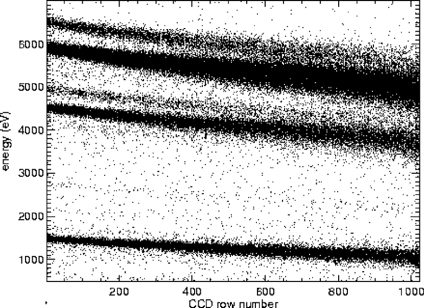
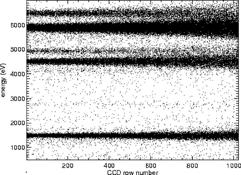
Figure 1: Upper panel: CTI in the I3 chip, illustrated with data from the ECS. Note the row-dependent gain and energy resolution and the energy-dependent charge loss. Lower panel: CTI-corrected version of these data.

CTI redistributes the charge in each event among the pixels in the 3$\times$3 island (grade “morphing”) as some charge traps release their charge on short timescales, so that charge reappears in adjacent pixels. This grade morphing, coupled with the standard g02346 grade filtering, causes the QE to vary with event energy and position on the device.

We have developed and optimized a model of CTI that accounts for charge loss and the spatial redistribution of charge (“trailing”), in both the parallel and serial registers, thus reproducing the spatially-dependent gain, QE, and grade distribution of these devices. By forward modeling of these effects separately for each event, we produce a “CTI-corrected” event list that is useful for data analysis and astrophysical interpretation.

For the BI devices, we must model parallel and serial charge loss and trailing independently to match the data. There are charge traps in the imaging array, framestore array, and serial register. Since the FI devices were damaged by radiation that penetrates only a few microns into the device (Prigozhin et al., 2000), their (shielded) framestore arrays and serial registers are protected. So, although the CTI is more pronounced on FI devices, it is easier to model than in the BI devices. Our techniques are described in more detail, with more emphasis on the BI devices, in a separate article (Townsley et al., 2000).

2 The Model

Our CTI model is phenomenological, characterizing the effects of CTI in the data rather than directly modeling the spatial distribution and time constants of the trap population (see Gallagher et al. (1998) and Krause et al. (1999) for examples of such physical models). The charge lost and trailed into the adjacent pixel are given by $L=k_{1}C^{k_{2}}$; $T=k_{3}L^{k_{4}}$ where $C$ is the charge in a single pixel, $L$ is the charge lost per pixel transfer, $T$ is the charge trailed per pixel transfer, and the $k$’s are the CTI parameters. We chose power law functional forms for these relations because they adequately fit the data and ensure zero charge loss or trailing when there is zero charge present. The parameters $k_{1}$–$k_{4}$ are determined by fitting lines to pixel amplitude versus x and y chip positions for many energies. Examples of each of these fits are shown in Townsley et al. (2000). To apply CTI to a given event, these equations are calculated for each pixel in the event, then the resulting numbers are multiplied by the number of pixel transfers to determine how much charge to remove from each pixel in the event. The trailed charge is then added back into the appropriate adjacent pixel.

Note that our model is “local” – prediction of the amount of charge lost by a particular event does not consider the possibility that another event falling in the same columns but closer to the amp will have filled some portion of the traps, reducing the charge loss from its nominal value (Gendreau et al., 1995). We do however consider shielding effects that may occur within the nine pixels of a single event. For example, an isolated pixel of height 1000 Data Numbers (DN, the digital units of charge output by ACIS, $\simeq$4 eV) will encounter more empty traps (suffer more loss) than a pixel of height 1000 DN that is immediately following a pixel of height 400 DN. The “leading” pixel’s charge is sacrificed to fill the traps encountered by the event, shielding the 1000 DN pixel. Thus we apply our loss model only to the portion of the pixel’s charge that is larger than its predecessor’s. In this example, the 1000 DN pixel will suffer loss and trailing approximately the same as a 600 DN isolated pixel. Details of the shielding model are given in Townsley et al. (2000).

Although ACIS FI devices do not exhibit serial CTI, they do show a small charge loss effect which is proportional to the distance between the CCD pixel and the left or right edge of the CCD. This is believed to be caused by the slight drop in clocking voltages suffered between the middle of the CCD and the supply leads at the chip edges (M. W. Bautz, private communication). CTI scales the effect so that these gain variations are row-dependent, with the bottom rows of the chip showing virtually no variation and the top rows varying by up to $\sim$100 DN at high energies ($\sim$6 keV). We model this gain variation for each amp as a linear function of distance from the readout node, averaging over all rows.

To account for nonlinearities not modeled directly by the fits described above, we also incorporated a “CTI deviation map” into our model that refines the CTI for each event’s specific location on the chip. This map is produced by examining the residual gain variations left after the basic model is applied. By correcting ECS data with and without this deviation map, we have determined that including it improves the final results. See Townsley et al. (2000) for details.

3 The Corrector

Having modeled CTI, we can try to remove its effects from actual ACIS events, taking a forward-modeling approach. For each observed event, we first hypothesize the nine pixel values of a corresponding true event, i.e. the event that would have been obtained if no CTI effects were present. This true event is passed through the CTI model, producing a model event. The hypothesis is then adjusted pixel-wise by adding the difference between observed event and model event to true event and repeating the process. This iterative adjustment continues until model event and observed event differ by less than one DN, at which point true event constitutes the CTI-corrected event.

The performance of the corrector in removing the observed spatial variation of event energy in ECS data is shown in the lower panel of Figure 1. The corrector has largely removed the gain changes across the device. Since the spectral broadening with row number is primarily the result of a random process involving one of the trap species (Antunes et al., 1993), it cannot be suppressed in our reconstructed events.

The success of the CTI corrector in regularizing the grade distribution at the top of an FI device is shown in Table 1, combining a broad range in energies (0.5–7 keV) made up of the Al, Ti, and Mn calibration lines. For example, 43.6% of events migrated from grade 2 to grade 0 during CTI correction.

Table 1: Correcting Grade Migration in ECS Data

	original grade								new distribution
new grade	0	1	2	3	4	5	6	7	top	bottom
0	9.3	0.0	43.6	0.0	0.0	0.0	0.0	0.0	52.9	49.7
1	0.0	0.0	0.1	0.0	0.0	0.2	0.0	0.1	0.4	0.3
2	0.0	0.0	11.3	0.0	0.0	0.0	0.0	0.0	11.3	16.0
3	0.0	0.0	0.0	0.3	0.3	0.2	4.7	0.0	5.5	6.0
4	0.0	0.0	0.0	0.3	0.3	0.1	4.6	0.0	5.3	5.9
5	0.0	0.0	0.0	0.0	0.0	0.3	0.3	0.3	0.9	0.5
6	0.0	0.0	0.0	0.0	0.0	0.0	7.2	4.1	11.3	13.5
7	0.0	0.0	0.0	0.0	0.0	0.0	0.0	12.3	12.3	8.0

Note. — For events falling at the top of the detector (rows 824:1024) where CTI is most severe, Columns 2–9 show the percentage of events having a certain ASCA grade before correction (table column) and a certain ASCA grade after correction (table row). Entries in boldface represent events gained by CTI correction; entries underlined represent events lost, assuming the standard g02346 grade filtering. Column 10 shows the corrected grade distribution at the top of the detector. For comparison column 11 shows the corrected grade distribution at the bottom of the detector (rows 1:201). Summing down Columns 2–9 would give the grade distribution at the top prior to correction.

Table 1 demonstrates an improvement in QE after CTI correction. Figure 2 illustrates this in more detail. For low-energy events (e.g. Al K) the charge is more spatially concentrated, leading to more single-pixel events. CTI causes these to morph into grades that are still captured in the standard grade filtering, so the QE at the top of the device is not affected by CTI. At higher energies (e.g. Mn K) events are often intrinsically split, so grade morphing causes them to be lost to ASCA-like grade 7. The corrector can recover some of these events, but clearly the QE is still row-dependent. This is due in part to telemetry constraints: certain ACIS grades are not transmitted to the ground because they are primarily cosmic ray events and would saturate telemetry. When CTI causes legitimate photon events to grade morph into these grades, they are lost forever. Other events are not recovered into their original grades because the corrector is unable to recover charge that has been eroded by CTI down below the split threshold – at that level, the charge is indistinguishable from noise and the corrector is purposely not allowed to include such pixels in its reconstruction. Note that the bottom quarter of the device is largely unaffected by the CTI degradation and thus retains the original performance of the detector.

Figure 2: Relative QE at Al K (bottom) and Mn K (top) across the I3 device, before (dashed lines) and after (solid lines) CTI correction, ASCA g02346 only. The binsize is 32 rows. For Al K, corrected and uncorrected QE are nearly identical. Uncorrected Mn K data show $\sim$19% fewer events at the top of the device than at the bottom; corrected data show a modest QE improvement but still $\sim$11% fewer events at the top of the device compared to the bottom.

The CTI corrector consists of a set of IDL (Research Systems Inc.) programs and parameter files that instantiate the model for each amplifier on each CCD, for a given epoch of the Chandra mission. The code is available (www.astro.psu.edu/users/townsley/cti/corrector/) and may be of interest to other groups concerned with the results of radiation damage on X-ray and optical CCD detector systems. This website is intended to provide an example of the corrector, not an exhaustive and complete set of correction code immediately applicable to any dataset.

4 Model Uncertainties

The FI corrector must be optimized to match the CTI present at the time of the observation in question, since the CTI has changed over the course of the mission. This can be achieved by tuning the corrector’s parameters on the ECS dataset taken most closely in time to the target observation. There is an uncertainty introduced by using calibration data to tune this or any other model: we must assume that the CTI measured by the ECS is representative of that present in celestial data. Most ACIS events are due to particle interactions and are not even telemetered. It is primarily these events that fill traps and thus regulate CTI. Since most of these particle events are from cosmic rays that are not stopped by the Observatory structure, it is reasonable to assume that ECS and celestial data have comparable particle fluxes, thus a comparable trap population.

We have used the instrumental Au L$\alpha$ (9.7 keV) and Ni K$\alpha$ (7.5 keV) lines as rough diagnostics of the corrector’s performance on celestial data. Tests show that the corrector works fairly well even at these high energies (well above the energies used to tune it), reducing the charge loss per pixel transfer by a factor of $\sim$10. Better results might be obtained by hybridizing the corrector optimization process to include both celestial and ECS data.

Another implication of tuning the corrector to ECS data is that we have no calibration information below Al K$\alpha$ (1.486 keV). Understanding the behavior of the CCDs between 0.2 and 1.5 keV is important for obtaining accurate hydrogen column densities, comparing ACIS results to ROSAT results, and inferring valid astrophysics for the large number of soft sources Chandra will examine. As a preliminary example, we consider the supernova remnant E0102-72.3, used as a soft calibration source for Chandra. The CXC provided us with two calibration datasets on this target (N. Schulz, private communication), one with the target near the readout of Node 2 on the I3 chip (“obsid 49”) and a second with the target half-way up the chip (“obsid 48”), on the same node. An observation with the target near the top of the chip is scheduled and will be included in subsequent analysis.

These data were obtained in January 2000 but CTI-corrected with the code tuned to ECS data obtained the previous September. Even though the corrector was not tuned below 1.486 keV and was based on the CTI present 4 months prior to the E0102-72.3 observations, the corrected data for both observations showed the soft lines in this source at the correct energies to within $\pm$1% above 800 eV and to within $\pm$2% between 500 and 800 eV. The grade distributions before and after correction were identical, to within statistical uncertainties, for obsid 49. Grade migration was noticeable in the raw data from obsid 48. CTI correction restored the grade distribution to values consistent with obsid 49. With future data we hope that E0102-72.3 can be used to calibrate the corrector as well as to check it.

The uncertainties outlined above should encourage ACIS users to treat their data with care and caution. This is especially important for public calibration targets observed before mid-September 1999, as the CTI was changing rapidly then.

5 Astrophysical Implications

Users of ACIS data must be aware of CTI and its spatial and spectral effects in order to generate astrophysically relevant results. Without CTI correction, accurate analysis of ACIS data requires a strongly position-dependent response matrix (“.rmf file”) and QE map (part of the “.arf file”). These of course depend on the user’s choice of grade filtering; it is not clear that the usual ASCA-like grade filtering is optimal for sources far from the readout nodes.

Our CTI corrector improves the photon energy estimates and significantly corrects for grade morphing. The corrector also improves the energy resolution of the ACIS devices more than can be achieved by only accounting for the row-dependent gain variations. Using these features, we recover linewidths in the External Calibration Source data that are on average 10% narrower (for both FI and BI detectors) than parallel gain detrending alone can provide.

These features mean that CTI-correcting ACIS event lists will yield several benefits for the end user. Correcting for grade morphing yields more high-energy counts and thus gives deeper source detection for hard sources; since most source-finding algorithms rely on a threshold number of counts to constitute a detection, adding even a modest number of counts can increase the number of detections significantly. For example, $\sim$15% more hard (2–8 keV) sources were detected in the ACIS GTO observations of the Hubble Deep Field and surroundings after CTI correction (Hornschemeier et al., 2000). Corrected event energies are necessary to obtain valid hardness ratios for faint point sources and to compare the spectral properties of faint sources distributed across a field. Improved energies and more uniform QE will also yield better spectrally-resolved imaging of extended sources, an important technique for studying supernova remnants, for example.

The corrector cannot totally eliminate the position-dependent energy resolution of the FI devices or the energy- and position-dependent QE. Thus position-dependent response matrices and effective areas are still necessary for the most accurate spectral fitting and flux determinations.

The CXC provides a tool (“MKRMF”) that allows the user to generate spatially-dependent .rmf files for spectral analysis of CTI-affected data. In principle, we might use this tool for ACIS spectroscopy while still benefiting from the CTI corrector. As an example, the event list should be CTI-corrected before any grade filtering is applied, since the corrector can ameliorate grade morphing. Then the standard g02346 grade filtering will yield an event list containing valid X-ray events that is larger than that obtained by filtering on the original event list. Selecting these events out of the original event list will give the best subset of events for spectral analysis. The MKRMF tool is then still applicable, as the observer will be using the original event list. Such a method might be useful for spectral analysis of moderately faint sources, where including additional photons would improve the spectral fits.

Also necessary for spectral fitting is the “MKARF” tool that incorporates the CCD QE into the .arf files. Currently, MKARF overestimates the high-energy QE for FI devices, since it presumes pre-launch values. This will lead to underestimates of the high-energy flux, corrupting the temperatures or spectral indices obtained in model fits. It should be possible, though, to treat CTI-induced QE changes as an energy-dependent multiplicative correction to the .arf file after it is generated, for either original or CTI-corrected data.

For even more detailed spectro-spatial analysis, especially for extended sources, we have incorporated our CTI model into the Monte Carlo simulator that we developed to model ACIS devices (Townsley et al., 2000). Work is ongoing (G. Chartas, private communication) to couple this CCD model with astrophysical models from XSPEC (Arnaud, 1996) and raytracing via MARX (Wise et al., 1997). This will eventually allow complete forward modeling to reproduce the data and optimize spectral fitting results.

Efforts continue throughout the entire Chandra community to improve the performance of the ACIS devices and our understanding of that performance. We expect the methods described here to be useful for current data but eventually to be superceded for future data by modifications to the instrument operations and software that are under development now at MIT. Laboratory work by MIT (Prigozhin et al., 2000) and PSU (Hill et al., 2000) scientists is yielding new insight into the damage mechanisms and providing data useful for calibrating and assessing mitigation techniques. In the meantime, our CXC colleagues are providing tools for coping with CTI-affected data and suggesting observing strategies that allow most ACIS users to accomplish their basic science goals.

References

- Antunes et al. (1993) Antunes, A., Burrows, D. N., Garmire, G. P., Lumb, D. H., & Nousek, J. A. 1993, Experimental Astronomy, 4, 159
- Arnaud (1996) Arnaud, K. A. 1996, in ADASS V, ASP Conf. Ser. 101, 17
- Bautz et al. (1998) Bautz, M., et al. 1998, SPIE, 3444, 210
- Burke et al. (1997) Burke, B., Gregory, J., Bautz, M., Prigozhin, G., Kissel, S., Kosicki, B., Loomis, A., & Young, D. 1997, IEEE Trans. Electron. Devices, 44
- Gallagher et al. (1998) Gallagher, D. J., Demara, R., Emerson, G., Frame, W. W., & Delamere, A. W. 1998, SPIE, 3301, 80
- Gendreau et al. (1995) Gendreau, K. C., Prigozhin, G. Y., Huang, R. K., & Bautz, M. W. 1995, IEEE Transactions on Electron Devices, 42, 1912
- Hill et al. (2000) Hill, J. E., et al. 2000, SPIE, 4012, in press
- Hornschemeier et al. (2000) Hornschemeier, A. E., et al. 2000, ApJ, submitted
- Krause et al. (1999) Krause, N., Briel, U. G., Dennerl, K., Soltau, H., Strueder, L., & Zavlin, V. E. 1999, SPIE, 3765, 220
- O’Dell & Weisskopf (1998) O’Dell, S. L., & Weisskopf, M. C. 1998, SPIE, 3444, 2
- Prigozhin et al. (2000) Prigozhin, G., Kissel, S., Bautz, M., Grant, C., LaMarr, B., Foster, R., & Ricker, G. 2000, SPIE, 4012, in press
- Townsley et al. (2000) Townsley, L. K., Broos, P. S., & Nousek, J. A. 2000, Nucl. Instr. and Meth. in Phys. Res. A, in preparation
- Townsley et al. (2000) Townsley, L. K., Broos, P. S., Nousek, J. A., Pavlov, G. G., Moskalenko, E., Chartas, G., & Rabban, L. W. 2000, Nucl. Instr. and Meth. in Phys. Res. A, in preparation
- Wise et al. (1997) Wise, M. W., Davis, J. E., Huenemoerder, D. P., Houck, J. C., Dewey, D., Flanagan, K. A., & Baluta, C. 1997, The MARX 2.0 User Guide, http://chandra.harvard.edu
- Yamashita (1995) Yamashita, A. 1995, Master’s thesis, University of Tokyo