Three-dimensional modelling of edge-on disk galaxies

Abstract

We present detailed three-dimensional modelling of the stellar luminosity distribution for the disks of 31 relatively nearby ($\leq$ 110 Mpc) edge-on spiral galaxies. In contrast to most of the standard methods available in the literature we take into account the full three-dimensional information of the disk. We minimize the difference between the observed 2D-image and an image of our 3D-disk model integrated along the line of sight. Thereby we specify the inclination, the fitting function for the z-distribution of the disk, and the best values for the structural parameters such as scalelength, scaleheight, central surface brightness, and a disk cut-off radius. From a comparison of two independently developed methods we conclude, that the discrepancies e.g. for the scaleheights and scalelengths are of the order of $\approx 10\%$. These differences are not due to the individual method itself, but rather to the selected fitting region, which masks the bulge component, the dust lane, or present foreground stars. Other serious limitations are small but appreciable intrinsic deviations of real disks compared to the simple input model.
In this paper we describe the methods and present contour plots as well as radial profiles for all galaxies without previously published surface photometry. Resulting parameters are given for the complete sample.

1 Introduction

Global parameters of galactic disks can be used to constrain the formation process as well as the evolution of disk galaxies. Recently it has become possible to deduce parameters such as scalelength or central surface density from numerical or semi-analytical self-consistent galaxy formation models (Syer et al. syer (1999), Mo et al. mo (1998), Dalcanton et al. dal (1997)) and compare the results with observed values. Observationally the Hubble Deep Field gives the opportunity to study morphological features and simple structural parameters for galaxies even at high redshifts (Takamiya taka (1999), Marleau & Simard hdfmorph (1998), Fasano & Filippi fasan (1998)).
Former statistical studies providing sets of homogeneously derived parameters for nearby galaxy samples are those of de Jong (1996b ) using a two-dimensional and of Courteau (cour (1996)) with a one-dimensional decomposition technique.
However, so far only a few statistical studies based on high quality CCD data (de Grijs dgmn (1998), Barteldrees & Dettmar bd (1994), hereafter Paper I) have addressed the actual three-dimensional structure of disk galaxies with regard to the stellar distribution perpendicular to the plane (z-direction) and taking into account an outer truncation (cut-off radius) for the disk, first introduced by van der Kruit & Searle (1981a ).
While the stellar distribution perpendicular to the plane (z-profile) could result from various ”heating” processes during the galactic evolution (Toth & Ostriker toth (1992), Hernquist & Mihos hern (1995)), the cut-off radius can be used to constrain either the angular momentum of a protocloud (van der Kruit vdk87 (1987)) or possible starformation thresholds in the gaseous disk (Kennicutt kenni (1989)).
In the following, we have compiled parameters of galactic disks for a total of 31 edge-on galaxies in different optical filters of which 17 objects have been already discussed in Paper I. One goal of our detailed comparison of several independent fitting procedures is to study the influence of the applied techniques on resulting disk parameters. It also provides the data base for statistical analysis addressing some of the above mentioned questions (e.g., Pohlen et al. pol (2000)). For 14 objects surface photometric data are given for the first time in Appendix A.

2 Observations and data reductions

2.1 Observations

The observations were carried out at the 42-inch (1.06m) telescope of the Lowell Observatory located on the Anderson Mesa dark side during several nights in December 1988 (run identification: L1) and January 1989 (L2) and at the 2.2m telescope at ESO/La Silla during three runs in June 1985 (E1), March (E2) and June (E3) 1987. At the 42-inch telescope we used a 2:1 focal reducer with the f/8 secondary, equipped with a CCD camera which is based on a thinned TI 800x800 WFPC 1 CCD with 15 $\mu$m pixelsize resulting in a field of approximately 9$\arcmin$ with a scale of 0.7$\arcsec$pixel^-1. Images were taken with a standard Johnson R filter. Observations at the 2.2m telescope were carried out with the ESO CCD adapter using a 512x320 RCA chip, giving an effective field size of $\approx 3\arcmin\;$x$\;2\arcmin$ and a scale of 0.36$\arcsec$pixel^-1. For the ESO observing runs we used the g, r, and i filters of the Thuan and Gunn (tg (1976)) system. Exposures were mainly taken in the g or r band, and only seven galaxies were observed in all three filters.

2.2 Sample selection

The northern sample observed at Lowell was selected automatically in an electronic version of the UGC-catalog (Nilson ugc (1973)) searching for galaxies with an inclination class 7 matching the field size. After visual inspection to check the inclination and remove interacting and disturbed galaxies, the observed sample was chosen out of the remaining galaxies according to the allocated observing time.
For the southern sky there is no comparable catalog providing information of inclinations directly. Using the axial ratios given e.g. in the ESO-Lauberts & Valentijn catalog (lv (1989)) will introduce a selection bias preferring late type galaxies with lower B/D ratio (Guthrie guthri (1992), Bottinelli et al. bot (1983)). One way to avoid this is extending the first selection to much lower axis ratios, comparable to $i\approx 65\degr$, and then checking the inclination by eye. Therefore we selected the galaxies according to the field size of about $2\arcmin$ from a visual inspection of film copies of the southern sky survey (see Paper I).
Table 1 gives a list of the resulting sample used during our fitting process, with a serial number (1), the principal galaxy name (2), the used filter (3), the integration time in minutes (4), and the run identification label (5), whereas the ’$\star$’ marks images already published in Paper I. Further parameters are taken from the RC3 catalogue (de Vaucouleurs et al. rc3 (1991)): the right ascension (6) and declination (7), the RC3 coded Hubble-type (8), the Hubble parameter T (9), and the D₂₅ diameter in arcminutes (10). In the case of ESO 578-025 parameters are taken from the ESO-Uppsala catalogue (Lauberts eso (1982)).

Table 1: Global parameters of sample galaxies with models

No.	name	filter	$t_{int.}$	run	RA	DEC	RC3	T		D25		$v_{\sun}$	D
			[min]	ID	(2000.0)		type			[$\;\arcmin\;$]		km s-1	Mpc
(1)	(2)	(3)	(4)	(5)	(6)	(7)	(8)	(9)		(10)		(11)	(12)
1	ESO 112-004	r	40	E3$\star$	002804.2	$-$580611	.S.R6*.	5.	6	1.	32	—	—
2	ESO 150-014	r	20	E3$\star$	003637.9	$-$565424	.L..+*/	-0.	7	1.	91	8257	107.	05
3	NGC 585	R	20	L1	013142.5	$-$005555	.S..1*/	1.	0	2.	14	5430	72.	15
4	ESO 244-048	r	15	E3	013908.8	$-$470742	.S..3./	3.	0	1.	38	6745	87.	09
5	NGC 973	R	10	L1	023420.2	+323020	.S..3..	3.	0	3.	72	4853	66.	28
6	UGC 3326	R	30	L1	053936.0	+771800	.S..6*.	6.	0	3.	55	4085	57.	82
7	UGC 3425	R	30	L1	061442.0	+663400	.S..3..	3.	0	2.	51	4057	57.	04
8	NGC 2424	R	15	L1	074039.8	+391359	.SBR3*/	3.	0	3.	80	3113	43.	10
9	IC 2207	R	10	L2	074950.8	+335743	.S..6*.	6.	0	2.	04	4793	65.	10
10	ESO 564-027	r	30	E2	091154.4	$-$200703	.S..6*/	6.	3	4.	07	2177	26.	93
11	ESO 436-034	g	60	E3$\star$	103244.2	$-$283646	.S..3./	3.	0	2.	09	3624	46.	02
12	ESO 319-026	g	30	E3$\star$	113020.0	$-$410357	.S..5./	5.	3	1.	48	3601	45.	32
12	ESO 319-026	i	30	E3
12	ESO 319-026	r	30	E2
12	ESO 319-026	r	30	E3$\star$
13	ESO 321-010	g	30	E3$\star$	121142.2	$-$383253	.S..0*/	0.	0	1.	86	3147	39.	53
13	ESO 321-010	r	30	E3$\star$
14	NGC 4835A	r	40	E3$\star$	125713.6	$-$462243	.S..6*/	6.	0	2.	57	3389	42.	54
15	ESO 575-059	r	15	E2	130744.5	$-$192348	.LA.+?/	-0.	8	1.	86	4570	59.	78
16	ESO 578-025	g	30	E2	140815.5	$-$200019	—	1.	0	1.	60	6364	83.	93
16	ESO 578-025	g	30	E3$\star$
16	ESO 578-025	i	30	E2
16	ESO 578-025	r	30	E2
17	ESO 446-018	r	30	E2	140838.7	$-$293412	.S..3./	3.	0	2.	34	4774	62.	15
18	IC 4393	r	30	E2	141749.5	$-$312056	.S..6?/	6.	0	2.	40	2754	35.	15
19	ESO 581-006	r	30	E3$\star$	145803.1	$-$192329	.SBS7P/	7.	0	1.	70	3119	40.	91
20	ESO 583-008	r	30	E3	155750.5	$-$222947	.S?….	6.	0	1.	51	7399	97.	98
21	UGC 10535	r	25	E2	164600.0	+062800	.S..2..	2.	0	1.	10	7586	102.	48
22	NGC 6722	r	10	E3$\star$	190339.6	$-$645341	.S..3./	3.	0	2.	88	5749	73.	79
23	ESO 461-006	r	60	E3$\star$	195155.9	$-$315852	.S..5./	5.	0	1.	62	5949	78.	26
24	IC 4937	g	20	E1	200518.0	$-$561520	.S..3./	3.	0	1.	95	2337	28.	68
24	IC 4937	i	20	E1
24	IC 4937	r	30	E3$\star$
25	ESO 528-017	g	30	E3$\star$	203320.8	$-$270549	.SB.6?/	5.	7	1.	59	6115	80.	73
25	ESO 528-017	i	30	E3
25	ESO 528-017	r	60	E3$\star$
26	ESO 187-008	r	30	E3$\star$	204325.2	$-$561217	.S..6./	6.	0	1.	51	4412	56.	31
27	ESO 466-001	i	40	E3	214232.3	$-$292210	.S..2./	2.	0	1.	38	7068	93.	13
28	ESO 189-012	g	60	E3$\star$	215538.7	$-$545233	.SA.5*/	5.	0	1.	66	8398	109.	04
28	ESO 189-012	i	20	E3
28	ESO 189-012	r	30	E3$\star$
29	ESO 533-004	r	20	E1	221403.2	$-$265618	.S..5*/	4.	8	2.	34	2594	33.	54
30	IC 5199	g	30	E3$\star$	221933.0	$-$373201	.SA.3*/	3.	0	1.	55	5061	65.	78
30	IC 5199	i	30	E3
31	ESO 604-006	r	30	E3$\star$	231454.0	$-$205944	.S..4./	4.	0	1.	86	7636	100.	92
$\star$ marks images already published in Paper I

2.3 Data reduction

We applied standard reduction techniques for bias subtraction, bad pixel correction and flatfielding. Following the procedure described in Paper I the sky background was fitted for each image using the edges of the individual frames to reduce any large scale inhomogeneity in the field of view. For part of the data we tried to remove the foreground stars from the image, but even with sophisticated PSF fitting using IRAF-DAOphot routines we were not able to remove stars without any confusion. The remaining residuals were always of the order of the discussed signal. This technique could only be used to mask out the regions affected by stars. In order to increase the signal-to-noise ratio near the level of the sky background part of the data was filtered using a weighted smoothing algorithm (see Paper I). Thereby the noise was reduced by about one magnitude measured with a three sigma deviation on the background, whereas the interpretation of the faint structure is hampered by this process.
We therefore conclude that the best way is to omit any additional image modifications, besides a rotation of the image to the major axis of the disk.

2.4 Photometric calibration

Most of the images were taken during non-photometric nights, therefore we tried a different way to perform photometric calibration. Comparing simulated aperture measurements with published integrated aperture data led to the best possible homogeneous calibration of the whole sample. Most of the southern galaxies were calibrated using the catalogue of Lauberts & Valentijn (lv (1989)), whereas NED was used for all northern galaxies. We used equation (1) derived in Paper I for the colour transformation of R and B literature values and the g measurements, and no correction between the R and r, and I and i band, respectively. Due to the fact that the photometric errors, of the input catalogues from Lauberts & Valentijn (lv (1989)) as well as within the RC3 catalogue (de Vaucouleurs et al. rc3 (1991)) are of the order of $0.1$ mag, we do not apply any further corrections. Galaxies calibrated in this way are marked with l in column (5) of Table 2, whereas for galaxies which did not have published values for their magnitude in the observed filter, we interpolated from calibrated images of the same night, by comparing the count rates for the sky value. These galaxies are marked with an i. For a few nights no galaxy with published photometry was observed and in these cases we used interpolated night sky values from the same observing run. Images calibrated in this way are marked with e in Table 2. The resulting zero points and central surface brightness values in these cases should be interpreted carefully, although the derived structural parameters, like scalelength and scaleheight, are not influenced by any uncertainty in the flux calibration.
Appendix A shows the contour plots and selected radial profiles for the 14 objects (25 images) not already published in Paper I.

2.5 Distance estimates

In order to derive the intrinsic values of the scale parameters and to compare physical dimensions we tried to estimate distances for our galaxies. Therefore we took published radial velocities corrected for the Virgo centric infall from the LEDA database, and estimated the distance following the Hubble relation with a Hubble constant of $H_{0}\!=\!75$ km s^-1Mpc^-1. Table 1 gives the heliocentric radial velocities (11) according to LEDA, and our estimated distances (12).

3 Disk models

3.1 Background

Our disk model is based upon the fundamental work of van der Kruit and Searle (1981a , 1981b , 1982a , 1982b ). They tried to find a fitting function for the light distribution in disks of edge-on galaxies. These galaxies are, compared to the face-on view, preferred for studying galactic disks due to the fact, that in this geometry it is possible to disentangle the radial and vertical stellar distribution. Their model include an exponential radial light distribution found for face-on galaxies (de Vaucouleurs, devau59 (1959); Freeman, free (1970)), a sech² behaviour in $z$, which is expected for an isothermal population in a plan-parallel system (Camm, camm (1950); Spitzer, spitzer (1942)), and a sharp edge of the disk, first observed by van der Kruit (vdk79 (1979)) in radial profiles of edge-on galaxies. The resulting luminosity density distribution for this symmetric disk model is (van der Kruit & Searle 1981a ):

$$\hat{L}(R,z)=\hat{L}_{0}\ \exp{\left(-\frac{R}{h}\right)}\ {\rm sech}^{2}{\left(\frac{z}{z_{0}}\right)}\qquad R<R_{\rm co}$$ (1)

$\hat{L}$ being the luminosity density in units of [$L_{\sun}$ pc^-3], $\hat{L}_{0}$ the central luminosity density, $R$ and $z$ are the radial resp. vertical axes in cylinder coordinates, $h$ is the radial scalelength and $z_{0}$ the scaleheight, and $R_{\rm co}$ is the cut-off radius.
The empirically found exponential radial light distribution is now well accepted and it is proposed that viscous dissipation could be responsible (Firmani et al. firmani (1996), Struck-Marcel struck (1991); Saio & Yoshii saio (1990), Lin & Pringle lp (1987)), although there is so far no unique explanation for the disk being exponential. An alternative description of the form $1/R$ proposed by Seiden et al. (seiden (1984)) did not get much attention, although it emphasizes the empirical nature of the exponential fitting function.
To avoid the strong dust lane and to follow the light distribution down to the region $z\!\approx\!0$ Wainscoat (wain (1986)) and Wainscoat et al. (wainetal (1989)) carried out NIR observations using the much lower extinction in this wavelength regime compared to the optical. They found a clear excess over the isothermal distribution and proposed the z-distribution to be better fitted by an exponential function $f(z)\!=\!\exp(-z/z_{0})$. According to van der Kruit (vdk88 (1988)) such a distribution would led to a sharp minimum of the velocity dispersion in the plane, which is not observed (Fuchs & Wielen fw (1987)). Therefore he proposed $f(z)\!=\!{\rm sech}(z/z_{0})$ as an intermediate solution. De Grijs (dg (1997)) extended this to a family of density laws $g_{m}(z,z_{0})\!=\!2^{-2/m}\ g_{0}\ {\rm sech}^{2/m}\left(mz/2z_{0}\right)(m>0)$ following van der Kruit (vdk88 (1988)), where the isothermal ($m=1$), and the exponential ($m=\infty$) cases represent the two extremes.
Therefore the luminosity density distribution can be written as:

$$\hat{L}(R,z)=\hat{L}_{0}\ \exp{\left(-\frac{R}{h}\right)}\ f_{n}(z,z_{0})\ {\rm H}(R_{\rm co}-R)$$ (2)

with H$(x_{0}-x)$ being the Heaviside function.
In order to limit the choice of parameters we restrict our models to the three main density laws for the z-distribution (exponential, sech, and sech²). Due to the choice of our normalised isothermal case $z_{0}$ is equal to $2h_{z}$, where $h_{z}$ is the usual exponential vertical scale height:

$$f_{1}(z) = 4\ \exp{\left(-2\ \frac{\mid z\mid}{z_{0}}\right)}$$

$$f_{2}(z) = 2\ {\rm sech}\left(\frac{2z}{z_{0}}\right)$$

$$f_{3}(z) = {\rm sech}^{2}{\left(\frac{z}{z_{0}}\right)}$$

In contrast to Paper I and Barteldrees & Dettmar (bdold (1989)) we define the cut-off radius at the position where the radial profiles become nearly vertical, corresponding to the mathematical description. They tried to avoid any confusion due to the lower signal-to-noise in the outer parts, by fixing the cut-off radius where the measured radial profile begin to deviate significantly from the pure exponential fit.

3.2 Numerical realisation

The model of the two dimensional surface photometric intensity results from an integration along the line of sight of the three dimensional luminosity density distribution (2) with regard to the inclination $i$ of the galaxy. Describing the luminosity density of the disk in a cartesian-coordinate grid K($x$-$y$-$z$) with $R=\sqrt{(x^{2}+y^{2})}$ leads to the following coordinate transformation into the observed inclined system K^′($x^{\prime}$-$y^{\prime}$-$z^{\prime}$) with $x^{\prime}$ pointing towards the observer, whereas the rotation angle between the two systems corresponds to $90\degr-i$:

$$x = x^{\prime}\sin(i)-z^{\prime}\cos(i)$$

$$y = y^{\prime}$$

$$z = x^{\prime}\cos(i)+z^{\prime}\sin(i)$$

Taking into account this transformation we have to integrate equation (2), obtaining an equation for the intensity of the model disk depending on the observed radial and vertical axes $y^{\prime}$ and $z^{\prime}$ on the CCD:

$$I(y^{\prime},z^{\prime})=\int\limits_{-\infty}^{+\infty}\hat{L}\bigl{(}x(x^{\prime},z^{\prime},i),y^{\prime},z(x^{\prime},z^{\prime},i)\bigr{)}dx^{\prime}$$ (3)

Together with equation (2) this gives:

$$I(y^{\prime},z^{\prime})=\qquad\qquad\qquad\qquad\qquad\qquad\qquad\qquad\qquad$$

$$\hat{L}_{0}\int\limits_{-\infty}^{+\infty}\!\!\exp{\left(-\frac{\sqrt{(x^{\prime}\ \sin i-z^{\prime}\ \cos i)^{2}+y^{\prime 2}}}{h}\right)}f_{n}(z^{\prime},z_{0})$$

$$\ast\,{\rm H}\left(R_{\rm co}-\sqrt{(x^{\prime}\ \sin i-z^{\prime}\ \cos i)^{2}+y^{\prime 2}}\right)\>dx^{\prime}\quad$$ (4)

Therefore six free parameters fit the observed surface intensity on the chip ($y^{\prime}$, $z^{\prime}$ plane) to the model:

$$I=I(y^{\prime},\ z^{\prime},\ i,\ n,\ \hat{L}_{0},\ R_{\rm co},\ h,\ z_{0})$$ (5)

Figure 1 shows a sequence of computed models with an isothermal z-distribution ($n\!=\!3$) for the exact edge-on case ($i\!=\!90\degr$) with characteristic values for the ratio $R_{\rm co}/h$: $1.40,2.88,5.00$ and for $h/{z_{0}}$: $2.0,4.0,7.3$ keeping the cut-off radius $R_{\rm co}$ and the total luminosity $L_{tot}\!\propto\!zh^{2}\hat{L}_{0}$ constant. The latter is causing a different central surface brightness $\mu_{0}$ for each model, ranging from 23.8 to 19.3 starting with $\mu_{0}\!=\!21.2$ mag$/\squareforqed\arcsec$ for the reference model with $R_{\rm co}/h\!=\!2.88$ and $h/{z_{0}}\!=\!4.0$. All contour lines falling within the interval $\mu\!=\!25.0$ – $19.5$ are plotted with a spacing of 0.5.

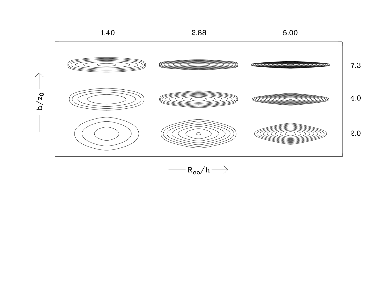
Figure 1: Different galaxy models computed according to equation (4) with constant values for the ratio $\frac{R_{\rm co}}{h}$ within the columns, or $\frac{h}{z_{0}}$ within the rows, whereas $\hat{L}_{tot}$ and $R_{\rm co}$ are constant for all models using an isothermal description for the exact edge-on case

3.3 Method 1

3.3.1 Determination of fitting area

The first step is to divide the galaxy into its quadrants. The four images are then averaged according to their orientation, following van der Kruit & Searle (1981a ) and Shaw (s93 (1993)). Thereby larger foreground stars and asymmetrical perturbations in the intensity distribution are eliminated by omitting this region during averaging. Smaller foreground stars are removed by median filtering. The average quadrant should result at least from three quadrants to get a representative image of the galaxy. This averaging additionally increases the signal-to-noise ratio. In order to determine the fitting area for modelling the disk component on the final quadrant, one has to avoid the disturbing influence of the bulge component and the dust lane. The region dominated by the bulge is fixed following Wyse et al. (wgf (1997)) defining the bulge component by “light that is in excess of an inward extrapolation of a constant scale-length exponential disk”. Therefore the clear increase of the intensity towards the center which can be seen in radial cuts determines an inner fitting boundary $R_{\rm min}$. We tried to minimize the dust influence (cf. Section 4.4.2) by placing a lower limit $z_{\rm min}$ in the vertical direction by visual inspection. Additionally we restricted the remaining image by a limiting contour line $\mu_{\rm lim}$, where the intensity drops below a limit of 3$\sigma$ on the background.
We are aware of the problem that these are rather rough definitions difficult to reproduce without quoting the exact values for $R_{\rm min},z_{\rm min},\mu_{\rm lim}$. However, the final choice of the fitting area is a complex and subjective procedure depending on the intrinsic shape of each individual galaxy, the influence of their environment, and the quality of the image itself. Therefore it is not possible to quote exact general selection criteria and to derive the structural parameters straight forward. One solution is to do it in a consistent way for a large sample, leaving the problem of comparing results from different methods (cf. Section 4.2).

3.3.2 Numerical fitting

The numerical realisation of the fitting procedure minimizes the difference ($SQ$) between the averaged quadrant and a modelled quadrant based on equation (4).

$$SQ=\sum_{j}\Bigl{(}log\left(I_{O_{j}}(y_{j},z_{j})\right)-log\left(I_{M_{j}}(y_{j},z_{j})\right)\Bigr{)}^{2}$$

$I_{O_{j}}$ is the intensity within the average quadrant (observed intensity) and $I_{M_{j}}$ of the modelled intensity. In contrast to Shaw & Gilmore (sg89 (1989), sg90 (1990)) and Shaw (s93 (1993)) using a similar approach for their models we do not weight individual pixels. They weight the difference by the error in the surface brightness measure, which Shaw (s93 (1993)) derives from the averaging of the quadrants. However, this method implies an absolute symmetry for the disk in $z$ and $y$, which is not the case for real galaxies. These kind of errors only reflect the asymmetry of the galaxy. Using the observed errors in the surface brightness for weighting individual pixels does not result in a considerable advantage because they are nearly the same after smoothing. The minimal $SQ$ is found by varying five of the six free parameters of the model (cf. eq. 5), whereas the parameter $R_{\rm co}$ is determinated by cuts parallel to the major axis. A significant decrease of the intensity extrapolated to $I=0$ gives the value of $R_{\rm co}$ (van der Kruit & Searle, 1981a ), therefore it is important that the intensity at the cut-off radius is well above the noise limit. The other five parameters are determined by fixing the smallest $SQ$. For the three different functions $f(z)$ and every possible $i$ ($\Delta i=0.5\degr$) the remaining parameters ($\hat{L}_{0}$, $h$, and $z_{0}$) are varied with the “downhill simplex-method” (Nelder & Mead, nm (1965); Press et al., pftv (1988)) until the global minimum of $SQ$ is found. $I_{M_{j}}$ is calculated by a numerical gaussian integration of equation (4). The possible inclination angles can be restricted from the dust lane of the galaxy (Paper I). Tests of model disks with additional noise show that the “downhill simplex-method” found the input inclination $i$, the used model $f(z)$ and the other disk parameters within errors of $\delta h,\delta z_{0}$, and $\delta\hat{L}_{0}<$ 1%. An estimation of the errors of the parameters for the best model disk can be made by inspection of the parameter space for $SQ$ around the smallest $SQ$, with slightly different fitting areas, and different values of $R_{\rm co}$. $f(z)$ is in almost all cases the same and the variation of $i$ is only small ($\pm 1\degr$). The differences in $h$ and $z_{0}$ are about 15% (in some cases up to 25%), and $\hat{L}_{0}$ varies about a factor of 2.

3.4 Method 2

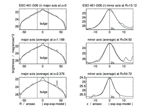
Figure 2: Example of the fitting procedure: Set of typical radial (left panel) and vertical (right panel) profiles used for the fitting process of the galaxy ESO 461-006 together with the model.

Within this method all disk parameters as well as the choice of the optimum function $f(z)$ are estimated by a direct comparison of calculated and observed disk profiles by eye.
As a first step, the inclination $i$ is determined by using the axis ratio of the dust lane. Depending on the shape of the dust lane it is possible to restrict the inclination to $\pm 1.5\degr$. The central luminosity density $\hat{L}_{0}$ is calculated automatically for each new parameter set by using a number of preselected reference points along the disk. Given a sufficient signal-to-noise ratio, the cut-off radius $R_{\rm co}$ can be determined from the major axis profile. Thus, the remaining fitting parameters are the disk scale length and height, $h$ and $z_{0}$, as well as the set of 3 functions $f(z)$. The scale length $h$ is fitted to a number (usually between 4 and 6) of major axes profiles (left panel of Fig. 2). The quality of the fit for the vertical profiles along the disk can be used as a cross-check for the estimated scalelengths (right panel of Fig. 2). The disk scaleheight $z_{0}$ is estimated by fitting the $z$-profiles, outside a possible bulge or bar contamination. The vertical disk profiles of most of the galaxies investigated enable a reliable choice of the quantitatively best fitting function $f(z)$. This is due to the fact that the deviations between different functions become visible at vertical distances larger than that of the most sharply-peaked dust regions. The first raw fitting steps are usually carried out by using a reduced number of both major and minor axis profiles simultaneously. Afterwards, when a good first fitting quality is reached, a complete set of major and minor calculated and observed axes profiles are investigated in detail. At the end of this procedure a final, complete disk model is calculated using all previously estimated disk parameters.

4 Results

4.1 Distribution of disk parameters

Table 2 contains the best fit model for each image. Together with the galaxy name (1), the filter (2), and the referring image (3), with integration time, and run ID, we list the inclination (4), the best fitting function for the z-distribution (5), the calibration index (6) (ref. Section 2.4), and the central surface brightness of the model (7), without correcting for inclination. According to the distance tabulated in Table 1, the cut-off radius $R_{\rm co}$ (8) is given in kpc and arcsec as well as the scalelength $h$ (9) and the vertical scaleheight $z_{0}$ (10) which is normalised to the isothermal case, being two times an exponential scaleheight $h_{z}$. For the seven galaxies with available images in more than one filter, we do not see any correlation of fitted parameters with different wavelength, although we find the same inclination angle for the best fitted disk within the range of the errors. Appendix A shows the best fitting model as an overlay to selected radial profiles for each image. The subsequent analysis of the distribution for the different parameters concerning the formation and evolution of galaxies will be given in forthcoming papers.

Table 2: Determined parameters set

galaxy	filter	image	$i$		$f(z)$	cali.	$\mu_{0}$	$R_{\rm co}$					$h$					$z_{0}$
			[$\degr$]				mag$/\squareforqed\arcsec$	[$\;\arcsec\;$]		[kpc]			[$\;\arcsec\;$]		[kpc]			[$\;\arcsec\;$]		[kpc]
(1)	(2)	(3)	(4)		(5)	(6)	(7)	(8)					(9)					(10)
ESO 112-004	r	40E3	87.	5	sech	l	21.14	45.	0	—			22.	7	—			2.	8	—
ESO 150-014	r	20E3	90.	0	sech	l	22.00	64.	1	33.	27		23.	4	12.	14		5.	5	2.	85
NGC 585	R	20L1	88.	0	sech	e	21.76	70.	0	24.	49		32.	7	11.	44		10.	6	3.	71
ESO 244-048	r	15E3	87.	0	$\exp$	l	20.54	45.	4	19.	17		13.	7	5.	78		7.	2	3.	04
NGC 973	R	10L1	89.	5	$\exp$	e	20.83	105.	0	33.	74		51.	5	16.	55		12.	4	3.	99
UGC 3326	R	30L1	88.	0	sech2	e	21.50	101.	5	28.	45		70.	4	19.	74		4.	7	1.	32
UGC 3425	R	30L1	87.	0	sech2	e	21.01	80.	5	22.	26		29.	2	8.	08		7.	4	2.	05
NGC 2424	R	15L1	86.	5	$\exp$	e	20.52	112.	0	23.	40		31.	7	6.	62		11.	9	2.	49
IC 2207	R	10L2	86.	5	$\exp$	e	21.04	56.	0	17.	67		38.	2	12.	06		6.	7	2.	12
ESO 564-027	r	30E2	88.	0	sech	l	21.11	140.	4	18.	33		50.	9	6.	65		6.	6	0.	86
ESO 436-034	g	60E3	88.	0	sech	l	20.96	82.	1	18.	32		22.	6	5.	04		6.	8	1.	52
ESO 319-026	g	30E3	86.	5	sech	e	21.51	60.	1	13.	21		14.	2	3.	12		3.	1	0.	68
ESO 319-026	r	30E2	86.	0	$\exp$	i	21.14	63.	0	13.	84		14.	7	3.	23		3.	2	0.	70
ESO 319-026	r	30E3	88.	0	sech2	i	21.94	61.	9	13.	60		13.	2	2.	90		2.	8	0.	62
ESO 319-026	i	30E3	88.	0	sech	l	21.01	64.	8	14.	24		14.	3	3.	14		3.	4	0.	75
ESO 321-010	g	30E3	88.	0	sech	l	20.11	64.	4	12.	34		19.	9	3.	81		4.	7	0.	90
ESO 321-010	r	30E3	88.	0	sech	l	19.54	64.	8	12.	42		21.	6	4.	14		5.	0	0.	96
NGC 4835A	r	40E3	85.	5	$\exp$	l	20.92	90.	0	18.	56		40.	4	8.	33		7.	9	1.	63
ESO 575-059	r	15E2	87.	0	sech2	l	20.78	60.	5	17.	53		22.	6	6.	55		6.	4	1.	86
ESO 578-025	g	30E2	86.	5	$\exp$	l	21.58	50.	7	20.	63		17.	0	6.	92		7.	5	3.	05
ESO 578-025	g	30E3	86.	5	$\exp$	l	21.69	50.	7	20.	63		17.	0	6.	92		7.	5	3.	05
ESO 578-025	r	30E2	86.	0	$\exp$	l	21.02	50.	4	20.	51		14.	9	6.	06		7.	4	3.	01
ESO 578-025	i	30E2	86.	0	$\exp$	l	20.27	47.	5	19.	33		20.	3	8.	26		7.	6	3.	09
ESO 446-018	r	30E2	86.	5	sech	l	20.45	75.	6	22.	78		23.	7	7.	14		3.	9	1.	18
IC 4393	r	30E2	87.	0	$\exp$	l	20.30	75.	6	12.	88		29.	8	5.	08		5.	8	0.	99
ESO 581-006	r	30E3	86.	5	$\exp$	l	21.33	55.	8	11.	07		18.	2	3.	61		5.	6	1.	11
ESO 583-008	r	30E3	87.	0	$\exp$	i	20.84	56.	2	26.	70		14.	0	6.	65		3.	8	1.	81
UGC 10535	r	25E2	88.	0	sech2	i	21.50	41.	4	20.	57		11.	4	5.	66		4.	3	2.	14
NGC 6722	r	10E3	86.	5	sech	l	19.47	86.	0	30.	77		21.	6	7.	73		6.	2	2.	22
ESO 461-006	r	60E3	87.	5	$\exp$	l	20.96	61.	6	23.	37		21.	1	8.	01		3.	8	1.	44
IC 4937	g	20E1	88.	5	sech2	l	22.73	74.	9	10.	41		93.	8	13.	04		5.	6	0.	78
IC 4937	r	30E3	88.	0	sech2	l	21.29	83.	5	11.	61		32.	1	4.	46		5.	9	0.	82
IC 4937	i	20E1	88.	5	sech	e	19.92	78.	1	10.	86		38.	6	5.	37		7.	2	1.	00
ESO 528-017	g	30E3	86.	5	$\exp$	l	21.98	57.	6	22.	54		20.	5	8.	02		3.	5	1.	37
ESO 528-017	r	60E3	86.	5	$\exp$	l	21.28	55.	1	21.	56		19.	9	7.	79		2.	7	1.	06
ESO 528-017	i	30E3	86.	5	sech	l	20.89	50.	0	19.	57		22.	6	8.	85		3.	2	1.	25
ESO 187-008	r	30E3	85.	5	$\exp$	l	20.77	50.	0	13.	65		15.	1	4.	12		4.	4	1.	20
ESO 466-001	i	40E3	87.	0	$\exp$	e	19.52	52.	6	23.	76		13.	0	5.	87		8.	2	3.	70
ESO 189-012	g	60E3	87.	0	$\exp$	l	21.50	56.	2	29.	81		26.	8	14.	21		3.	8	2.	02
ESO 189-012	r	30E3	86.	5	$\exp$	l	20.71	56.	5	29.	97		20.	6	10.	93		3.	4	1.	80
ESO 189-012	i	20E3	87.	0	sech	l	20.44	54.	7	29.	01		22.	7	12.	04		3.	2	1.	70
ESO 533-004	r	20E1	88.	0	$\exp$	l	20.32	68.	4	11.	12		33.	1	5.	38		7.	7	1.	25
IC 5199	g	30E3	86.	5	$\exp$	l	21.55	64.	1	20.	44		19.	9	6.	35		5.	6	1.	79
IC 5199	i	30E3	86.	5	$\exp$	l	19.97	57.	6	18.	37		19.	9	6.	35		4.	9	1.	56
ESO 604-006	r	30E3	90.	0	sech	l	21.22	70.	6	34.	54		27.	9	13.	65		3.	8	1.	86

4.2 Comparison of different methods

The different fitting methods were independently developed within two diploma theses (Lütticke 1996, Schwarzkopf 1996). The quality of the data basis for each project was the same. From the sample presented here there were five objects in common. These are used to compare the two methods and determine the quantitative difference of the derived parameters.

Table 3: Comparison of the different determined parameter sets for the same galaxy images

galaxy	$f(z)$	$i$	$z$	$h$	$R_{\rm co}$
		[$\;\degr\;$]	[$\;\arcsec\;$]	[$\;\arcsec\;$]	[$\;\arcsec\;$]
	sech	88.0	5.0	21.6	64.8
ESO 321-010 r {	$\exp$	88.0	5.2	25.9	64.1
	$\exp$	87.5	3.8	21.1	61.6
ESO 461-006 r {	$\exp$	87.5	3.6	16.2	61.2
	$\exp$	86.5	6.1	26.8	83.5
IC 4937 r {	sech	89.5	7.0	27.4	75.6
	$\exp$	86.5	3.2	19.3	56.2
ESO 189-012 r {	$\exp$	88.0	3.6	21.3	56.9
	sech	88.5	4.1	39.8	67.7
ESO 604-006 r {	sech2	89.5	3.2	24.5	73.4

Table 3 shows the results for the five images. The mean deviation in the determined inclination is $\approx\!1\degr$ and 12.4% for the scaleheight (ranging from 5.0%-26.6%) whereas for three images different functions for the z distribution were used. The mean difference for the radial scalelength is 20.6% (2.1%-47.2%) and 4.2% for the determination of the cut-off radius.
A subsequent analysis shows that it is not possible to ascribe the sometimes quite large discrepancies to the quality of the individual method. It turns out, that the main problem is the non-uniform determination of the fitting area. The intrinsic asymmetric variations of a real galactic disk compared to the model enforce a more subjective restriction of the galaxy image to the fitting region, whereby for example one has to exclude the bulge area and the dust lane.
This finding is in agreement with the study of Knapen & van der Kruit (knap (1991)) who compared published values of the scalelength and find an average value of 23% for the discrepancy between different sources. As already mentioned by Schombert & Bothun (sb (1987)) the limiting factor for accuracy of the decomposition is not the typical S/N from the CCD-telescope combination nor the errors in the determination of the sky background, but the deviation of real galaxies from the standard model.

4.3 Comparison with the literature

In our former study (Paper I) with an earlier method to adapt equation (4), 20 of our 45 galaxy images have already been used. We decided to re-use them in this study to get models for as many galaxies as possible in a homogeneous way. Additionally, Paper I only presents the best fit values for the isothermal model, and uses a different definition of the cut-off radius.
Only three galaxies are in common with the sample of de Grijs (dgmn (1998)): ESO 564-027, ESO 321-010, and ESO 446-018. The mean difference for the scalelength is 10.4 % (ranging from 1.2%-20.3%) and for the scale height (normalised to the isothermal case) 4.0% (0.0%-8.2%). For the remaining galaxies there are no models in the literature.

4.4 Model limitations

Our model only represents a rather simple axisymmetric three-dimensional model for a galactic disk, consisting of an one component radial exponential disk with three different laws for the density distribution in the z-direction and a sharp outer truncation. Therefore it does not include additional components, such as bulges, bars, thick disks, or rings, and cannot deal with any asymmetries. Features like spiral structure or warps are not included, whereas Reshetnikov & Combes (rescom (1998)) multiply their exponential disk by a spiral function introducing an expression to characterise an intrinsic warp depending on the position angle outside of a critical radius.
The choice of our fitting area tries to avoid the dust lane, possible only for almost edge-on galaxies, as a first step to account for the dust influence (cf. Section 4.4.2). Examples of models including a radiative transfer with an extinction coefficient $\kappa_{\lambda}(R,z)$ can be found in Xilouris et al. (xil99 (1999)). However, introducing more and more new components and features automatically increases the amount of free parameters. Therefore we restricted our model to the described six parameters, to obtain statistically meaningful characteristics for galactic disks.
In the following we demonstrate that a simple disk model omitting the bulge component and the dust lane give indeed reasonable parameters.

4.4.1 The influence of the bulge component

We have studied the influence of the bulge for some of our objects including the earliest type galaxy in our sample (ESO 575-059) presented here. We have subtracted our derived disk model from the galaxy and then tried to find the best representation for the remaining bulge by a de Vaucouleurs $r^{1/4}$ or an exponential model. Taking the slope of the vertical profile at $R\!=\!0$ and a fixed axis ratio, we have constructed the 2-dimensional model of the bulge. In agreement with Andredakis et al. (andre (1995)) we find, that bulges of early type galaxies are better fitted by an exponential profile than by a $r^{1/4}$. Figure 3 shows the resulting vertical and radial cuts for ESO 575-059 together with the models.

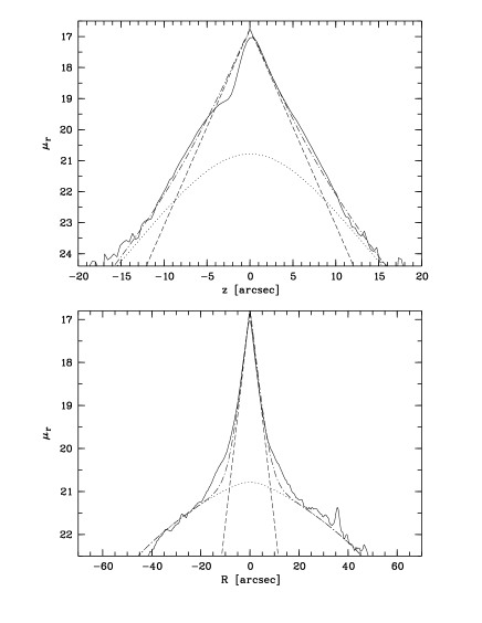
Figure 3: Minor and major axes profile for ESO575059r15E2 (solid lines) together with the best disk model (dotted), the best bulge model (dashed), and the resulting combined profile (dotted-dashed).

Despite the deviation between $R\!=\!10^{\prime\prime}$ and $R\!=\!20^{\prime\prime}$ which could be attributed to an additional component (inner disk or bar), we do not find any evidence for changing our disk model due to the influence of the bulge.
Therefore we conclude, that it is possible to nearly avoid any influence of the central component by fitting outside the clearly visible bulge region.

4.4.2 The influence of dust

Dust disturbs the light profile by a combination of absorption and extinction and the net effect has to be calculated by radiation transfer models. Therefore it is not obvious that outside the “visible” dust lane, which is excluded for the fitting area as a first step, the dust will not play a major role in shaping the light distribution. Xilouris et al. (xil99 (1999)), Bianchi et al. (simone (1996)), de Jong (1996a ), and Byun et al. (byun (1994)) have recently addressed this problem in more detail. Although they investigated the influence of the dust on the light distribution by quoting best fit structural parameters for the star-disk as well as the dust-disk, they did not quantify the influence on the star-disk parameters derived by standard fitting methods without dust. Even Kylafis & Bahcall (kylafis (1987)) state within their fundamental paper on finding the dust distribution for NGC 891 that “in order to avoid duplication of previous work, we will take … (the values for the star-distribution estimated by standard fitting methods)”.
We checked the influence of the dust on our determined parameter set, by studying simulated galaxy images with three different dust distributions. These dusty galaxies were kindly provided by Simone Bianchi who calculated images with known input parameters for the star and dust distribution with his Monte Carlo radiative transfer method (Bianchi et al. simone (1996)). We have defined a worst, best, and transparent case, according to the dust distributions presented by Xilouris et al. (xil99 (1999)), of our mean stellar disk ($R_{\rm co}\!=\!2.9$, $h/z\!=\!4$, and $f_{1}(z)$). The worst case is calculated with $\tau_{R}=0.51$, $h_{\rm d}/h_{\rm*}=1.55$, and $z_{\rm d}/z_{\rm*}=0.75$, the best case with $\tau_{\rm R}=0.20$, $h_{\rm d}/h_{\rm*}=1.08$, and $z_{\rm d}/z_{\rm*}=0.32$, and a transparent case without dust. To be comparable we used the same method for selecting the fitting region by masking the “visible” dust lane and reserving a typical area for a possible bulge component using mean values for the transparent case. In contrast to our standard procedure we do not restrict the inclination range from the appearance of the dust lane, but specify the best $SQ$ model in the range $i=80\degr\!-\!90\degr$ in Table 4. For the models marked with a ’$\star$’ we pretend the correct input inclination. Table 4 demonstrates, that even for the worst case we are able to reproduce the input parameters within the range of the typical 20% error discussed in Section 4.2. It should be mentioned that for each case we overestimate the input scalelength and -height, whereas the determination of $R_{\rm co}$ does not depend on the dust distribution. The implication on the distribution of the ratio $R_{\rm co}/h$ will be discussed in a forthcoming paper.

Table 4: Comparison of the results for the stellar disk (input: $z_{\rm*}\!=\!8.4$, $h_{\rm*}\!=\!33.7$, and $f(z)\!=$exp) from our fitting procedure for the three different dust distributions.

case	$i_{\rm in}$	$f_{n}$	$i_{\rm out}$	$z_{\rm*}$	$h_{\rm*}$	$\Delta z_{\rm*}$	$\Delta h_{\rm*}$
	[$\;\degr\;$]		[$\;\degr\;$]	[$\;\arcsec\;$]	[$\;\arcsec\;$]	[%]	[%]
trans.	87.5	1	87.5	8.5	34.0	$1.2$	$0.9$
best	85.0	1	84.5	8.5	35.0	$1.2$	$3.9$
best	87.5	1	86.5	8.6	35.5	$2.4$	$5.3$
best	90.0	1	87.0	8.7	36.0	$3.6$	$6.8$
best$\star$	90.0	1	90.0	8.8	35.0	$4.8$	$3.9$
worst	85.0	2	85.0	8.9	39.9	$6.0$	$18.4$
worst	87.5	2	86.0	8.8	39.1	$4.8$	$16.0$
worst	90.0	2	88.0	9.7	39.4	$15.5$	$16.9$
worst$\star$	90.0	2	90.0	9.8	39.1	$16.7$	$16.0$

4.5 Comments on individual galaxies

Trying to adapt a simple, perfect, and exact symmetric model to real galaxies always implies a compromise between the degree of any deviation and the final model (Section 4.6). The following list will provide some typical caveats found during the fit procedure which will characterise the quality of the specified model for individual galaxies.
ESO 112-004: warped, asymmetric, central part slightly tilted compared to disk, after fitting still remaining residuals
ESO 150-014: slightly warped, minor flatfield problems
NGC 585: remaining residuals
ESO 244-048: possible two component system, slope of inner radial profile significantly higher than of an outer one, final model fits the inner parts
NGC 973: one side disturbed by stray light of nearby star, seems to be radially asymmetric, remaining residuals
UGC 3425: superimposed star on one edge
NGC 2424: model does not fit very well without obvious reason
ESO 436-034: strong bulge component, possibly barred, hard to pinpoint final model, remaining residuals
ESO 319-026: outer parts show u-shaped behaviour, remaining residuals, therefore large ($\pm 2\degr$) difference in inclination angle
ESO 321-010: u-shaped, no clear major axis visible, therefore uncertain rotation angle, bar visible, bulge rotated against disk
NGC 4835A: strong residuals
ESO 446-018: the different sides of the disk are asymmetric visible in radial profiles and on the contour plot
IC 4393: similar to NGC 4835A
ESO 581-006: galaxy shows typical late type profile, $R_{\rm co}$ questionable, but nevertheless final model seems to fit well
ESO 583-008: disturbed by superimposed star, shows warp feature and a bar structure, $R_{\rm co}$ questionable, remaining residuals
UGC 10535: one side slightly extended
NGC 6722: only one side observed, bulge rotated against disk, barred, strongly disturbed by dust absorption, radial extension visible, therefore $R_{\rm co}$ should be treated with caution
ESO 461-006: minor flatfield problem seems to cause asymmetry, although model looks fine
IC 4937: similar to NGC 6722, dominating bulge, small disk, model significantly different compared to the i and r image, model possibly hampered by strong dust lane
ESO 578-025: bar visible
ESO 466-001: maybe two components, final model represents only inner part, outer part clearly different from normal disk component
ESO 189-012: slightly warped
ESO 533-004: similar to NGC 4835A, model fits the whole galaxy, leaving more or less no bulge component
IC 5199: slightly radial asymmetric
ESO 604-006: only one side observed, bar structure visible

4.6 Comments on some rejected galaxies

The model limitations described above constrain the application of our fitting process. Therefore we had to exclude about 20 galaxies from our original sample. They all show significant deviations from the simple geometry and an inclusion of their parameters obtained by forcing the model to fit the data will spoil the resulting parameter distribution.
One larger group classified mainly as S0 galaxies (e.g. NGC 2549, ESO 376-009, NGC 7332, ESO 383-085, ESO 506-033) shows a completely different behaviour of the luminosity distribution in the outer parts compared to the other galaxies. They all show an additional component, mainly characterised as an elliptical envelope. This is already visible in the contour plot, but becomes even more evident in a radial cut parallel to the major axis. In these cases the usual common curved decline of the profile (e.g. ESO 578-025) is missing, and is replaced by a more or less straight decline into the noise level, sometimes even by an upwards curved profile. Fitting these luminosity distribution by our one component exponential disk with cut-off, will therefore naturally provide parameters qualitatively different compared to late type disks. This will be discussed in detail in a forthcoming paper.
Another group consists of galaxies dominated mainly by their bulges, whereas the disk is only an underlying component, partly characterized as having thick boxy bulges (Dettmar & Lütticke db (1999)), e.g. IC 4745, ESO 383-005, although there are also pure elliptical bulges (e.g. ESO 445-049, NGC 6948).
In the case of ESO 383-048 and ESO 510-074 the radial profiles clearly indicate that a more complex model will be needed to fit these kind of multicomponent galaxies. Galaxies like UGC 7170 or ESO 113-006 were excluded due to their strong warps, which made it impossible to fit the model in a consistent way. Mainly late type galaxies such as ESO 385-008, IC4871, UGC 1281, or ESO 376-023 show a too patchy and asymmetric light distribution, that any attempt to fit the profiles will give only very crude, low quality parameters. UGC 11859 and UGC 12423 were rejected due to their thin faint disks, which will maybe overcome by taking new images with longer integration times to get a higher signal-to-noise ratio, whereas NGC 5193A is completely embedded into the surface brightness distribution of its near companion.

Appendix A Contour plots and radial profiles

The following figures show in the top panel selected cuts parallel to the major axis (full line) as well as the best fit model (dashed line) according to Table 2. The bottom panel shows isophote maps of the surface brightness for the galaxies, rotated to the major axis. The faintest plotted contour is defined by a 3$\sigma$ criterion of the background. Table 5 lists the name (1), image (2), and the vertical positions of the plotted profiles parallel to the major axes in arcsec (3). The contours are plotted equally spaced with 0.5 mag$/\squareforqed\arcsec$ starting from the limiting surface brightness $\mu_{{\rm lim.}}$ (4).

Table 5: Plotted parameters

galaxy	image	$z$	$\mu_{{\rm lim.}}$
		[$\;\arcsec\;$]	[mag$/\squareforqed\arcsec$]
(1)	(2)	(3)	(4)
NGC 585	R20L1	3,6,9,12	24.7
ESO 244-048	r15E3	$-$3,$-$9	24.8
NGC 973	R10L1	$-$2,$-$4,$-$6,$-$8	23.8
UGC 3326	R30L1	3,6,9	24.8
UGC 3425	R30L1	$-$1,$-$5,$-$9	24.2
NGC 2424	R15L1	1,3,5,7	24.5
IC 2207	R10L2	2,6,10	24.1
ESO 564-027	r30E2	2,4,6	25.2
ESO 319-026	i30E3	2,4,6	24.4
ESO 319-026	r30E2	2,4,6	24.7
ESO 575-059	r15E2	3,6,9	24.4
ESO 578-025	g30E2	2,4,6	25.2
ESO 578-025	i30E2	2,4,6	23.3
ESO 578-025	r30E2	2,4,6	24.5
ESO 446-018	r30E2	2,4,6,8	25.1
IC 4393	r30E2	$-$3,$\pm$6,$\pm$9	25.1
ESO 583-008	r30E3	2,4,6	25.0
UGC 10535	r25E2	2,4,6	25.5
IC 4937	g20E1	$-$2,$-$4,$-$6	25.1
IC 4937	i20E1	$-$2,$-$4,$-$6	23.3
ESO 528-017	i30E3	2,4,6	24.2
ESO 466-001	i40E3	1,3,5	23.8
ESO 189-012	i20E3	$-$1,$-$3,$-$5	24.1
ESO 533-004	r20E1	$-$3,$-$6,$-$9	24.6
IC 5199	i30E3	$\pm$2,$\pm$4,$\pm$6	23.8
remaining images already published in Paper I