The Search for Cosmological Black Holes:
A Surface Brightness Variability Test

Abstract

Recently it has been suggested that the majority of dark matter in the universe resides in the form of Jupiter mass black holes distributed cosmologically. This population makes itself apparent by microlensing high redshift quasars and introducing pronounced variability into their observed light curves. While several arguments dismissing this hypothesis have been presented, a conclusive observational test is, alas, sadly lacking. In this paper we investigate the effect of a cosmologically distributed population of microlensing masses on galaxies at low to intermediate redshift. The magnification of bright stars in these galaxies leads to small, but observable, fluctuations in their surface brightness. The variability time scale for Jupiter-mass lensing objects is of the order of a few months and this population may be detected through a future space-based monitoring campaign of a field containing $z\sim 0.5$ galaxies. The monitoring of galactic surface brightness will provide an effective test of the nature of dark matter on cosmological scales.

1 Introduction

The nature of dark matter is one of the major outstanding problems in current astrophysics, with the community being divided between two broad camps: those who propose particle dark matter and those who support massive compact objects. Both these ideas have received recent impetus due to the measurement of a neutrino mass (Fukuda et al., 1998) and the detection of MACHOs in the halo of our Galaxy (Alcock et al., 1993), although the small mass of the neutrino and the uncertainty in the location of the MACHO lenses suggests that the nature of majority of the dark matter still remains hidden from us.

One recent suggestion proposes that the variability seen in high redshift quasars, rather than being intrinsic to the source, is due to the microlensing action of Jupiter mass black holes distributed cosmologically along the line-of-sight to the quasar (Hawkins, 1993, 1996). To account for the characteristics of the variability, a substantial population of black holes is required, with a density high enough to account for a significant fraction of the total mass in the universe (Schneider, 1993). While there is theoretical support for such a model, with models of the quark-hadron transition producing black holes with a mass of $\sim 10^{-3}{\rm{\rm\,M_{\odot}}}$ [e.g. Hawkins & Taylor (1997)], observations have failed to reveal their presence in studies of the equivalent widths of distant quasars (Canizares, 1982; Dalcanton et al., 1994), although this conclusion has been contested (Hawkins, 1996). Other objections to this microlensing hypothesis have been raised (Baganoff & Malkan, 1995; Alexander, 1995), with corresponding rebuttals (Hawkins & Taylor, 1997). More recently, arguments have become quite vitriolic with the suggestion that this idea of cosmologically distributed black holes is being ignored by the astronomical community even though the apparent evidence is overwhelming (Hawkins, 1998).

The microlensing of cosmological supernovae provides a potential probe of any population of black holes (Schneider & Wagoner, 1987; Rauch, 1991, 1991a; Metcalf & Silk, 1999), although their rarity suggests that a long observational period may be required until an unambiguous detection is made. In this paper we provide a complementary probe of a cosmologically distributed black hole population; instead of supernovae as the source population, we focus here on microlensing on the much more numerous population of normal stars in galaxies out to ${\rm z\sim 0.5}$. In Section 2 we outline the analytic and numerical approach to this problem, while in Section 3 the results of a suite of simulations are presented. Section 4 is concerned with the time scale of the microlensing variability, and the observational feasibility of this study is discussed in Section 5. Section 7 presents the overall conclusions of this study.

2 Method

2.1 Background

Microlensing surveys of the Galactic halo focus upon identifying brightness fluctuations of a single, isolated source by an individual star or binary system along the line-of-sight (Paczynski, 1986). It is not necessary, however, to identify single stars in a search for microlensing. Proposing to search for MACHOs in the halo of M31, Crotts (1992) noted that while the light registered in a single pixel is a combination of the entire stellar population, the majority of it arises in a relatively small number of extremely luminous giants. In a stochastic manner a massive object in the halo of M31 will traverse the line-of-sight to a giant and induce a strong microlensing magnification, increasing the surface brightness of the entire pixel. A monitoring program of this ‘pixel lensing’ has recently come to fruition with the identification of several potential microlensing events (Crotts & Tomaney, 1996; Tomaney & Crotts, 1996; Alcock et al., 1999).

Given the relative lens geometry, however, the optical depth for such lensing is very small (${\rm 10^{-6}\rightarrow 10^{-5}}$), and events are extremely rare. Similarly, if all dark matter is in the form of MACHO-like objects distributed uniformly through-out the universe, the additional optical depth these would add in our view to M31 would, due to the small distance and hence low density of material, be negligible. Focusing instead out to intermediate redshift, however, the optical depth becomes more substantial (this is demonstrated below) and a number of microlenses will lie along our line-of-sight to a distant galaxy. In such a regime a fraction of the population of stars in a pixel will be subject to strong magnification. As the intrinsic motions of the microlensing objects change their positions with respect to the line-of-sight, the ‘state’ of the microlensing (i.e. how much each star is magnified) will also change, resulting in a fluctuation in the apparent luminosity of a patch of stars. The details of these fluctuations depends on several factors, including the optical depth to microlensing and the luminosity function of stars in the source galaxy; these are explored in more detail below.

2.2 Cosmological Considerations

Standard cosmological models assume that all material in the universe is smoothly and homogeneously distributed. In the following argument, however, all the matter in the universe is condensed in to compact objects. To begin with, it is assumed that these objects do not influence our line-of-sight view to a distant source. Dyer and Roeder (1972;1973;1974) considered the propagation of light through such an “empty beam” universe and found that the convergence, or focusing, of the beam is removed due to the lack of material and that objects at a particular redshift appear fainter than those observed in a universe where the matter is smoothly distributed, even the universal curvature is the same in both cases . For the purposes of this paper, we seek an intermediate position, with matter in the form of compact objects distributed randomly in the universe, with no constraint on their location with respect to our line-of-sight to a distant source. With this, the microlensing masses can influence the beam and, in the mean, the appearance of distant objects must be identical to that of a universe where all the matter is smoothly distributed (Weinberg, 1976). With respect to the empty-beam universe model, the influence of the lensing masses is to magnify the distant sources by a factor

$$\langle\mu_{th}\rangle(z)=\left[\frac{r_{1}(z)}{r(z)}\right]^{2}~{},$$ (1)

where $r(z)$ is the normalized angular diameter distance to a source at redshift $z$ in a universe with a smooth distribution of matter, and $r_{1}(z)$ is the equivalent distance in a universe with the same global value of $\Omega$, but with all the matter in the form of compact objects that do not influence the line-of-sight view to distant objects. These angular diameter distances are normalized such that $D(z)=(c/H_{o})r(z)$.

While the smooth matter case is analytically tractable, the solution of $r_{1}(z)$ typically requires the numerical solution of a differential equation (Dyer & Roeder 1972; 1973; 1974). In the following, however, we will assume that $\Omega=1$ and that all the matter is in the form of substellar compact objects. With these assumptions (Paczynski & Wambsganss, 1989);

$$\frac{r_{1}(z)}{r(z)}=\frac{3+z^{2}+2\sqrt{1+z}+z(3+\sqrt{1+z})}{5(1+z)}~{}.$$ (2)

While this tells us how bright objects will appear in the mean, the distribution of microlensing masses along any random line-of-sight will be different. This introduces a scatter in the brightness distribution and, as the relative positions of the microlensing masses and the source will change due to random motions of the lenses and sources, the magnification along any particular line-of-sight will vary with time. The first task is to determine the distribution of magnifications for a population of microlensing masses.

2.3 Microlensing

2.3.1 Microlensing Cross-Section

To determine the degree of microlensing-induced fluctuations on the surface brightness distribution of a distant galaxy, it is necessary to first derive the magnification ${\rm(\mu)}$ probability distribution for a source seen through a population of microlensing masses. This task is simplified by the fact that, irrespective of the mass spectrum of the microlenses, in the regime where $\mu$ is large, $p(\mu)\propto\mu^{-3}$ . In this case, the distribution is dominated by bright pairs of images and can be treated analytically [e.g. Schneider & Weiss (1988)]. At lower magnifications, however, the form of the magnification distribution function is strongly dependent upon the optical depth to microlensing, displaying complex secondary features due to higher order caustics (Rauch, Mao, Wambsganss & Paczynski, 1992; Wambsganss, 1992; Lewis & Irwin, 1995); no analytic treatment fully characterizing these low magnification features has been presented [although recent semi-analytical attempts have proved promising e.g. Kofman et al. (1997) & Lee et al. (1997)].

For the case of a single, isolated microlens mass the probability distribution of magnifications can be derived analytically (Schneider, Ehlers & Falco 1992) and is given by

$$p_{s}(\mu)~{}d\mu\propto\frac{d\mu}{(\mu^{2}-1)^{\frac{3}{2}}}~{}.$$ (3)

Note that this probability is independent of the mass of the lensing object. It is assumed that, in the regime relevant to this work, the microlensing optical depth is small, and the masses do not influence one another to produce complex caustic patterns. With these assumptions, the global magnification probability distribution is simply related to that of the isolated lensing mass.

2.4 Normalization

While Equation 3 presents the form of the magnification probability distribution, it still needs to be normalized before it can employed in any analysis. This question was addressed by Linder, Wagoner & Schneider (1988) who determined that in a universe with a global density $\Omega$, of which a fraction $1-\alpha$ is in the form of compact objects distributed randomly with a constant comoving density, then

$$p(\mu,z)= \frac{3}{2}\Omega(1-\alpha)\int^{z_{s}}_{0}dz~{}\frac{(1+z)}{\sqrt{1+\Omega z}}\left[\frac{r_{1}(z)}{r_{1}(z_{s})}\right]^{2}\times$$ (4)

$$\frac{r(z,z_{s})r(z_{s})}{r(z)}\int_{0}^{\infty}dm~{}\nu(m)p_{s}(\mu,m)~{},$$

where $\nu(m)$ is the mass spectrum of the lensing masses. The last integration in this expression reflects the fact that the maximum magnification a source can undergo is related to its physical size, the mass of the lensing objects and the lensing geometry (Chang & Refsdal, 1979). Here, $r(z_{1},z_{2})$ is the normalized angular diameter distance between two redshifts. For the gravitational lensing configurations presented in this paper, assuming a microlensing mass of $10^{-3}{\rm\,M_{\odot}}$ and considering the analysis of Chang (1984), $\mu_{max}\sim 100\rightarrow 200/\sqrt{R}$, where $R$ is the radius of the source star in Solar radii. The most luminous B and A stars have $R\sim 10R_{\odot}$, for which $\mu_{max}\sim 30\rightarrow 60$, while the stars contributing the majority of the populations luminosity possess $R\sim 1\rightarrow 10R_{\odot}$. This upper limit of the magnification cuts off the probability distribution function, slightly enhancing the distribution below $\mu_{max}$ [e.g. Figure 4 of Lewis and Irwin (1995)]. As significant magnification of stars can occur, we chose, therefore, not to restrict the probability distribution function. With this, Equation 3 is independent of the microlensing mass function, $\nu(m)$ can be replaced with an arbitrary $\delta$ function and Equation 4 can be used to derive a normalization, $k$, of the magnification probability distribution.

While Equation 4 provides a normalization, the magnification probability distribution as described by Equation 3 diverges as $\mu\rightarrow 1$; this is because in determining Equation 3 it is assumed that the lensing mass lies within an infinite plane, with which any finite impact parameter results in $\mu>1$. An infinite impact parameter is required for $\mu=1$. As we are limited to a finite amount of sky we require that $p(\mu)\rightarrow 0$ as $\mu\rightarrow 1$. We choose, therefore, to modify Equation 3 with a function to remove the divergence at $\mu=1$. The form employed is

$$p(\mu)=(1-e^{\mu_{w}(1-\mu)})^{2}\frac{k}{(\mu^{2}-1)^{\frac{3}{2}}}~{},$$ (5)

where both the values $\mu_{w}$ and $k$ are functions of redshift. This Equation is subject to two constraints, the first being the usual normalization of the probability distribution function, and the second being flux conservation between full and empty beam universes (Equation 1):

$$\int_{1}^{\infty}p(\mu)~{}d\mu=1$$ (6)

$$\int_{1}^{\infty}\mu~{}p(\mu)~{}d\mu=\langle\mu_{th}\rangle~{}.$$ (7)

However, as Equation 4 normalizes the asymptotic form of the probability distribution, the single free parameter in Equation 5, namely $\mu_{w}$, can be fixed with one of these equations, while the other can be employed to ensure consistency.

The procedure employed in this paper is to use Equation 6 to determine $\mu_{w}$. A series of these probability distributions, for source redshifts of $z=$ 0.1, 0.2, 0.3, 0.4 & 0.5, with $\Omega=1$ all in the form of compact objects, are presented in Figure 1, while Figure 2 presents $k$ and $\mu_{w}$ over the redshift range $z=0.05\rightarrow 0.5$. All of the magnification probability distributions possess a sharp peak near $\mu=1$, coupled with an asymptotic $p(\mu)\propto\mu^{-3}$ tail at high magnifications. These normalized distributions were then used to determine $\langle\mu\rangle$. This mean magnification is compared to the theoretically expected value (Equations 1 & 2) in Figure 3; there is an excellent agreement between the two approaches. This is due to the low optical depth (and hence simple) regime in which the analysis is undertaken, as at higher stellar densities, such as those responsible for the microlensing of multiply imaged quasars, individual stars no longer behave like isolated lenses and their combined effects can lead to extremely complex magnification patterns on a high redshift source (Wambsganss, Paczynski & Katz, 1990).

Considering the theoretically expected magnification it is simple to determine that the optical depth to microlensing out to the redshift of interest. This ranges from $\kappa_{*}\sim 0.002$ at $z=0.1$ to $\kappa_{*}\sim 0.04$ at $z=0.5$. These numbers are several orders of magnitude greater than the $\kappa_{*}\sim 10^{-6}\rightarrow 10^{-5}$ expected of gravitational microlensing in the Galactic halo and towards M31 [c.f. (Paczynski, 1986)], and hence, in this extragalactic scenario, microlensing effects should be more apparent. While these arguments demonstrate the efficacy of microlensing, deriving the detailed behavior requires knowledge of the underlying stellar luminosity function as the number density of potential sources will dictate the level of observed fluctuations in the stellar sample as a whole, a topic which we turn to in the next section.

How does Equation 5 compare to previous studies of the magnification probability distribution of microlenses distributed in three dimensions? The numerical studies undertaken by Rauch (1991;a) focus on substantially higher optical depths than those considered in this paper, although one case, with $\kappa_{*}=0.01$ [Figure 2 in Rauch (1991)], can be compared to distribution presented in Figure 1 for $z=0.2$ $(\kappa_{*}=0.008)$. An excellent correspondence between the two distributions can be seen over the entire magnification range. Kofman et al. (1997) and Lee et al. (1997) analytically tackled the form of the magnification probability distribution for both 2-D and 3-D distributions of microlensing masses. Also considering the numerical simulations of Rauch (1991;a) and Rauch et al. (1992), these papers investigate the nature of the higher order caustic features identified in the magnification probability distribution at large magnifications, features which are not accounted for in Equation 5. While substantially influencing the form of the 2-D distributions, these features were found to be very small for the corresponding 3-D distributions. The analysis of Kofman et al. (1997) and Lee et al. (1997) was not considered at the optical depths presented in this paper, but for $\kappa_{*}=0.1$ the caustic features induce a deviation of only $\sim 15\%$ at $\mu\sim 30$, where the distribution has fallen to $10^{-6}$ that of its peak value. At the optical depths considered in this paper, such deviations will be even more inconsequential, and can be ignored. Lee et al. (1997) comment on difficulty in determining the form of the magnification probability distribution at low magnifications, especially in the case where the microlensing masses are distributed in three dimensions. Comparing Figure 6 of Kofman et al. (1997) with Figure 13 of Lee et al. (1997), it can be seen that at small magnifications ($log_{10}(\mu)<0.1$) that the probability distributions for the 2-D and 3-D case are very similar. In this regime, Kofman et al. (1997) provide a semi-analytic formalism which approximates the form of the distribution. Comparing this to Equation 5 for the $z=0.5,\kappa_{*}=0.04$ case presented in this paper, a maximum difference of $\sim 7\%$ at $log_{10}(\mu)\sim 0.005$. Hence Equation 5 has an excellent correspondence with previous results.

2.5 Stellar Luminosity Function

With current instrumentation, the angular diameter of galaxies at redshifts of $z\sim 0.5$ ensures that they will extend over only a small number of pixels, and the light recorded in each pixel is the sum of the flux from a large number of stars. Each star in the pixel will be microlensed by some degree, and examining Figure 1, most stars will suffer a magnification $\mu\sim 1$, although a fraction of the population will be magnified by a much more substantial factor. On average, however, the overall flux in a pixel will be magnified by $\langle\mu_{th}\rangle$, although at any instant the brightness of a pixel will depend on the relative positions of the microlenses, as this dictates how much each star in the pixel is magnified. These will change due to the intrinsic velocity dispersion of the microlensing bodies, resulting in fluctuations in the observed flux within a pixel about this mean value. To be a useful probe of the intervening matter, however, these fluctuations must exceed some observable threshold. To properly determine this, the luminosity function of the source stellar population needs to be considered.

If the luminosity function is comprised of only relatively low luminosity stars then a large number is required to account for total flux detected in a pixel. When such a population is microlensed many stars will be in a highly magnified state. As the microlensing state changes, and the magnification of each star also changes, the absolute number of stars in the highly magnified state remains essentially constant. Even if a single star is extremely magnified, a very rare occurrence, then the contribution this star makes to the flux registered in a pixel is small compared to the overwhelming background of the numerous stars which are only moderately magnified. Conversely, if the luminosity function consists of only very luminous stars then only a small number are required to account for the luminosity in a pixel. It is very unlikely that any individual star is strongly magnified. When this rare event does occur, however, the contribution from the magnified star can dominate the flux received in a pixel, resulting in a substantial fluctuation in the observed surface brightness. The real situation, however, is a combination of the above and we expect that a stellar population sampled in a pixel consists of a large proportion of faint stars which are insensitive to the effects of microlensing, resulting in a background flux, and a relatively small number of very luminous stars which dominate the luminosity.

The luminosity function model we choose is the stellar LF from Jahreiß  and Wielen (1997), derived from Hipparchos data within $20{\rm\,pc}$ of the Sun. The characteristics of this luminosity function are presented in Figure 4; representing a population with a total luminosity of $10^{6}{\rm\,L_{\odot}}$, the solid line shows the number of stars possessing a luminosity greater than some value, while the dot-dashed line is their contribution to the total luminosity of the pixel. It is obvious from this picture that while stars with $L>10{\rm\,L_{\odot}}$ represent less than 1% of the population by number, they account for 70% of the total luminosity.

3 Magnification Distributions

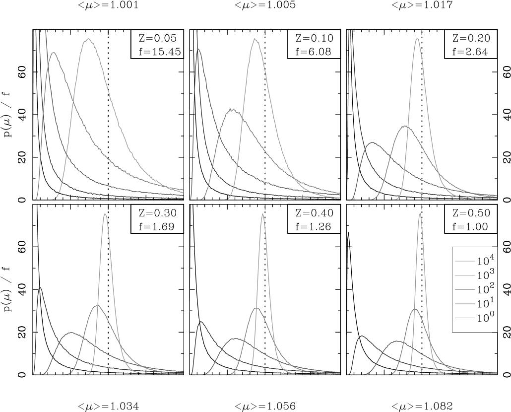
Figure 5: The distribution of the mean magnification of a sample of stars for redshifts between $z=0.05$ and $z=0.5$. The dotted vertical line represents the mean value of the relevant magnification distribution, while the lower bound on each plot is $\mu=1$. Each line consists of a stellar sample of 1, 10, 100, 1000 and 10000 stars, depending on its shading. The scale factor, f, is introduced such that all the curves can be placed on the same y-scale. As these are probability distributions, the integrated area under the curve (accounting for the f-scaling) is unity.

Given a population of microlensing masses, the magnification of a single star can be chosen by selecting from the magnification probability distribution given by Equation 5. For a sample of stars, magnifications can be drawn from this distribution multiple times to determine the total magnification of the population. While this is straight forward, it becomes computationally expensive when the population consists of a very large number stars. The procedure employed in this study is to determine the magnification statistics for various numbers of source stars, combining the results to reproduce the effect of microlensing the entire source stellar population. Analytically this can be calculated by convolving the magnification probability distribution for a single star (Equation 5) with itself $n_{samp}$ times, where $n_{samp}$ is the number of stars being microlensed. Again, while this is simple for a small population of source stars, the calculation becomes numerically unwieldy for a large number of stars. For the purpose of this paper, these statistics were generated a Monte Carlo approach, drawing $n_{samp}$ observations from Equation 5 and combining them to determine the mean magnification of the sample. Repeating this procedure $10^{6}$ times for each $n_{samp}$ it is then possible to determine the distribution of mean magnifications. The results of this sampling for several source redshifts between $z=0.05$ and $z=0.5$ are presented in Figure 5, with sample sizes ranging from 1 to $10^{4}$ source stars. At all redshifts the same trend is seen with the distribution of the means evolving from the single realization for (Equation 5) to a more Gaussian form as the sample size is increased; this is a consequence of the central limit theorem. These distributions can then be combined to determine the distributions of means for any sample size.

Armed with this information it is now possible to tackle the question of the overall brightness fluctuations expected for a population of stars drawn from a luminosity function, and hence the expected surface brightness fluctuation within a pixel. For this, the above magnification distributions are convolved with the stellar luminosity function described in Section 2.5, assuming a total luminosity, and hence number of stars in the population. Again, a Monte Carlo approach is taken and the luminosity function is binned logarithmically. While the bins at lower luminosity contain many stars they contribute a negligible fraction of the total luminosity and are uniformly magnified by $\left<\mu\right>$. At the high luminosity end, where the luminosity contributions of the bins become a more appreciable fraction of the total luminosity, magnification probability distribution for each bin is calculated by combining the appropriate population magnification probability distributions presented in Figure 5. The distribution for each bin is then combined, weighted by the luminosity fraction of the bin, to determine the magnification probability distribution for the entire population of stars. Two constraints, that the mean value of the final distribution must be $\left<\mu\right>$ and that the integrated area under the resultant probability distribution must be unity, are checked to ensure consistency. Figure 6 presents the results of this procedure for a range of source redshifts between $z=0.05$ and $z=0.5$, displaying the percentage variability for stellar populations of $10^{5}{\rm\,L_{\odot}}$ (dark grey), $10^{6}{\rm\,L_{\odot}}$ (medium grey) and $10^{7}{\rm\,L_{\odot}}$ (light grey) total luminosity. Table 1 presents the integral properties of these distributions with each column representing the range within which 10, 30, 50, 70 & 90% of the magnifications of the population lie, relative to the average magnification. A number of interesting features are immediately apparent; at low redshift the relatively small microlensing optical depth induces negligible fluctuations into the observed total brightness of any of the populations. This changes as the redshift, and hence the microlensing optical depth, is increased, until by redshift $z=0.5$ microlensing will introduce fluctuations of order $\sim 1\%$ into a sample with a total luminosity of $10^{5}{\rm\,L_{\odot}}$. Increasing the luminosity of the stellar sample, however, reduces the width of the distribution, as expected from the central limit theorem, such that a population of $10^{7}$ at $z=0.5$ will suffer fluctuations of $\lower 2.15277pt\hbox{$\;\buildrel<\over{\sim}\;$}0.5\%$. We turn to the observational aspects of such small variations in Section 5.

4 Event Timescales

While the magnification probability distribution is independent of the form of the underlying mass spectrum of lensing objects, the time-scale of any fluctuation depends implicitly on the mass of the microlenses. At the low optical depths considered here, any variability will be very simple in form, consisting of the superposition of isolated peaks rather than the complex light curves expected for high optical depth microlensing [e.g. Lewis, Miralda-Escude, Richardson & Wambsganss (1993)]. As with the microlensing of Magellanic Cloud sources, we can define a variability time-scale to be:

$$\tau = \frac{(1+z_{l})}{v}\left[\frac{4GM}{c^{2}}\frac{D_{ls}D_{ol}}{D_{os}}\right]^{\frac{1}{2}}$$ (8)

$$\approx 23.4\frac{(1+z_{l})}{v_{1000}}\left(\frac{M}{M_{\odot}}\right)^{\frac{1}{2}}\left[\frac{r(z_{l},z_{s})r(z_{l})}{r(z_{s})}\right]^{\frac{1}{2}}~{}h^{-\frac{1}{2}}~{}yrs~{},$$

where $M$ is the microlensing mass, $v_{1000}$ is the relative transverse velocity in units of $1000{\rm\,km\,s^{-1}}$, and $r(z_{1},z_{2})$ is the angular diameter distance.

For source galaxies out to $z\sim 0.5$, and considering a $10^{-3}{\rm\,M_{\odot}}$ microlensing mass, this time-scale is presented in Figure 7. The time-scale of the microlensing events are substantially less than a year for all lensing configurations and hence can be observed in a single observing season. When examining Figure 7, it is important to remember that the distribution of microlenses are volume-weighted (c.f. Equation 4), and hence are more likely to be located nearer to the source redshift. Similarly the typical time-scale for the microlensing events seen in the light curve of a population of stars will also be skewed to values less than the maximum seen in Figure 7. Detailed light curves are beyond the scope of this current paper and they will be the subject of a further study of this phenomenon.

5 Observational Considerations

5.1 Variability Detection

While the previous theoretical analysis has presented the framework for determining the effects of a cosmological population of microlensing masses, it is important to consider whether the amplitude of the expected variations are observable. Here we consider monitoring many distant galaxies simultaneously with a CCD detector, with resolution elements that each cover a population of luminosity $\sim 10^{7}{\rm\,L_{\odot}}$. Ignoring K-corrections, this corresponds to an apparent magnitude of $m=29.0$ at $z=0.5$ (assuming $q_{0}=0.5$ and $h=0.75$). It is immediately clear that such observations will normally be sky-limited, except for the Next Generation Space Telescope (NGST) for which the sky background is expected to be very low, and the spatial resolution high enough to have very small pixels.

To detect 1% variations at the $3\sigma$ level, 0.33% relative photometry is needed, that is, ${\rm S/N=333}$. Assuming an 8m diameter mirror, and a diffraction limited system, a count rate of $\sim 1.8S_{eff}$ photons/sec is expected from a $m=29.0$ object in the J-band with NGST, where $S_{eff}$ is the total system efficiency. For exposure times longer than a few minutes, such observations will be photon noise dominated, since a background of $<10^{-1}$ photons/sec/resolution element is expected at $1.1\mu m$. So the required $S/N$ is achieved in $17/S_{eff}$ hrs of exposure. For a population of stars at a redshift of $z\sim 0.5$ with a total luminosity of $10^{7}{\rm\,L_{\odot}}$, the probability of the necessary 1% variation is 4%, so several thousand such populations need to be monitored to detect a sample of microlensing events. (Although deeper observations, focusing upon the fainter regions of galaxies, will reveal similar scale fluctuations in $\sim 23\%$ and $\sim 56\%$ of the pixels for populations of, respectively, $10^{6}{\rm\,L_{\odot}}$ and $10^{5}{\rm\,L_{\odot}}$). Of course, in a typical field, many resolution elements on the CCD camera will cover $z\sim 0.5$ galaxies, and so the monitoring of the populations may be achieved simultaneously. If NGST is resolution limited, each resolution element will cover $0.001\Box{\mbox{\mbox{${}^{\prime\prime}$}}}$. For each resolution element to cover a $10^{7}{\rm\,L_{\odot}}$ population at $z\sim 0.5$, requires the observation of a region of surface brightness ${\rm 21.5mag/\Box{\mbox{\mbox{${}^{\prime\prime}$}}}}$. In regions fainter than ${\rm 21.5mag/\Box{\mbox{\mbox{${}^{\prime\prime}$}}}}$, boxes larger than a resolution element can be summed up, to give a total luminosity $10^{7}{\rm\,L_{\odot}}$; the variability of these boxes can also be studied with the penalty of a small amount of extra sky noise.

The HDF field shows that the area in a typical $2^{\prime}\times 2^{\prime}$ field covered by surface brightness ${\rm>21.5mag/\Box{\mbox{\mbox{${}^{\prime\prime}$}}}}$ regions of $z=0.5$ galaxies exceeds several tens of $\Box{\mbox{\mbox{${}^{\prime\prime}$}}}$, that is, tens of thousands of NGST resolution elements. The above cosmological microlensing-induced variability will be observed over a background of intrinsic variability events, due to supernovae, variable stars and galaxy self-lensing, as well as due to the inevitable Poisson noise in the observed counts. Unlike current studies of ‘surface brightness fluctuations’ method for distance determinations out to galaxies at $\sim 100Mpc$ (Tonry & Schneider, 1988; Thomsen, Baum, Hammergren & Worthey, 1997; Lauer, et al., 1998) which essentially requires single epoch observations, to identify microlensing induced variability a monitoring program is required, allowing the identification of supernovae by their light-curves and peak luminosities. Supernovae are also rare, as are variable stars with a luminosity sufficient enough to influence the total luminosity of populations $L\sim 10^{7}L_{\odot}$, if a survey was to focus on more luminous source pixels. As with supernovae, these would also reveal themselves via their characteristic light curves. If the depth of the survey is increased such that $L\sim 10^{5}L_{\odot}$ pixels are probed, the ubiquity of their variations would rule against variations in the source population. In the case of self-lensing of galaxy stars by MACHOs in the halo of the same galaxy provides a negligible contribution as the optical depth is many orders of magnitude smaller than that due to the cosmological microlenses considered here. The main source of detected background events is likely to be due to simple Poisson photon noise. However, in the situation outlined above, $3\sigma$ variations due to Poisson noise are approximately 40 times less common than the $3\sigma$ microlensing variations. Data at two epochs would allow an initial feasibility study. If the required variability rate is indeed observed, follow-up observations at further epochs should be taken to monitor the light curves of the variability events, to distinguish microlensing events from unlensed supernova or nova events, and to reject variations due to Poisson noise.

5.2 Extreme Events

The previous Section has demonstrated that the typical fluctuations in the brightness of a pixel is detectable and lends itself to future space-based observatories. But are there any aspects of microlensing by a cosmologically distributed population that would make them apparent with current technology? As noted earlier in this paper, while the vast majority of stars will be magnified by a value close to the theoretically expected mean (Equation 1), very rarely a star will undergo an extreme magnification. The probability that a particular star is magnified by an extreme value is found by integrating the magnification probability distribution (Equation 5), which is presented graphically in Figure 8. For instance, in a $10^{5}{\rm\,L_{\odot}}$ population, the LF of Figure 4 gives $\sim 0.1$ stars with $L\sim 10^{4}{\rm\,L_{\odot}}$; if such a star were to be magnified by a factor of 20, it would alter the surface brightness of the population by $200$%. At a redshift of $z=0.05$, this is an uncommon phenomenon, with probability $P(>\mu)=10^{-6}$, however, the apparent magnitude of the population is much brighter: $m=27.5$, and the photometric accuracy needed to resolve these variations is ${\rm S/N\sim 3}$. While these are within the range of HST’s capabilities, and many tens of fields of depth of $m=27.5$ with ${\rm S/N\lower 2.15277pt\hbox{$\;\buildrel>\over{\sim}\;$}3}$ have been reimaged, it is unlikely that a sufficient area has been covered to detect a sample of such rare events. So, while the tools are available, more substantial deep survey areas are required in a search for extreme events with HST.

6 Other Cosmological Models

While throughout this paper a standard flat cosmology with $\Omega_{o}=1$ has been employed, recent studies of high redshift supernovae suggest the presence of a substantial cosmological constant (Garnavich, et al., 1998). To investigate the influence of such a dominant cosmological constant on the result presented in this paper the formalism of light propagation in generalized Friedmann universes was employed (Linder, 1988). The full and empty beam distances in three universes were calculated in three cosmological models, $(\Omega_{o}=1,\Lambda_{o}=0)$, $(\Omega_{o}=0.3,\Lambda_{o}=0)$ and $(\Omega_{0}=0.3,\Lambda_{o}=0.7)$, used to calculate the mean relative magnification between the full and empty beam cases (Equation 1) and the microlensing optical depth. These are presented in Figure 9.

Out of these three models, the case presented in this paper consistently displays higher optical depth over the entire redshift range; this is simply due to the fact that in this model more material lies along the line of sight to a distant source. In comparison, the optical depth in the open case is several times smaller, reaching $\sigma\sim 0.15$ at $z=0.5$. The addition of a dominant cosmological constant into such a universe does not greatly change the values of the optical depths. This is because, while the cosmological constant changes the global curvature of the Universe, it has no influence on the Ricci focusing of the beam and locally the Universe appears as it is solely matter-dominated (it is for this reason that cosmological supernovae need to be identified at redshifts greater than 0.5 in an attempt to determine the geometry of the Universe).

7 Conclusions

Recent studies have claimed that the fluctuations observed in the light curves of high redshift quasars are due to the microlensing effect of a population of cosmologically distributed Jupiter mass black holes. While arguments have been presented to refute this claim, no observational test of this hypothesis has been readily available. In this paper we have investigated the effect this putative population would have on the surface brightness distribution of galaxies out to intermediate redshift. The results of this study conclusively demonstrate that if a significant population of cosmologically distributed compact objects are present, with enough mass to account for the universal dark matter budget, then they will induce a ‘twinkling’ into the observed surface brightness distributions of galaxies at low to intermediate redshifts. The magnitude of the observed fluctuations are a function of the redshift of the source galaxy, ranging from negligible values in the local Universe, to $\sim 1$% at $z=0.5$, with a time-scale of variability on the order of weeks to months.

While the optical depth to microlensing at such low to intermediate redshifts is still quite small and the induced fluctuations are at a relatively low level, the sky density of galaxies out to these redshifts vastly exceeds that of supernova and quasars, the current focus for the search for cosmologically distributed microlensing masses. With sufficiently deep imaging with source pixel luminosities of greater than $10^{5}L_{\odot}$, microlensing induced surface brightness variability can be detected over galaxies at intermediate redshifts, and the ubiquitous nature of this variability means it will dominate over any contaminating effects, such as supernovae, variable stars and self-lensing. The scale of the induced variability make observations conducive over a single observing season, and with the advent of the Next Generation Space Telescope, such observations will soon be possible. Hence, a monitoring program to search for fluctuations of the surface brightness of the plethora of galaxies at $z\lower 2.15277pt\hbox{$\;\buildrel<\over{\sim}\;$}0.5$ offers a effective test of the existence of cosmologically distributed compact matter.

8 Acknowledgements

We are grateful for discussions with Mike Hudson, Tom Quinn and Stephen Gwyn. The anonymous referee is thanked for useful comments.

Figure 1: Microlensing magnification probability distributions for $z=$ 0.1, 0.2, 0.3, 0.4 & 0.5. The corresponding microlensing optical depths are $\kappa_{*}=$ 0.002, 0.008, 0.017, 0.028 & 0.040 respectively.

Figure 2: The parameters $k$ (solid line) and $\mu_{w}$ (dashed line) for the magnification probability distribution (Equation 5) in the redshift range $z=0.05\rightarrow 0.5$.

Figure 3: A comparison between the theoretical value of the image magnification, $\langle\mu_{th}\rangle$, compared to that derived from the analytic approach presented in Section 2.

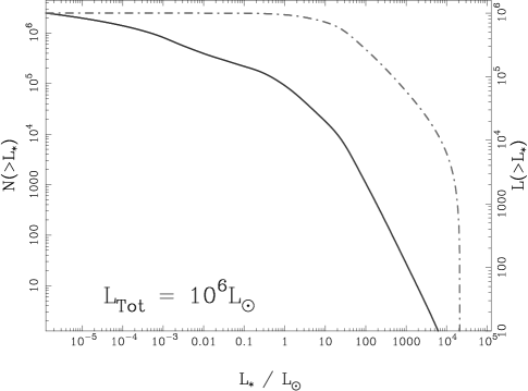
Figure 4: The properties of the assumed luminosity function, assuming a population with a total luminosity of ${\rm 10^{6}{\rm\,L_{\odot}}}$. The solid line represents the number of stars in the population with a luminosity greater that ${\rm L_{*}}$, while the dot-dash line is the summed luminosity of this subset of stars. While stars with ${\rm L>10{\rm\,L_{\odot}}}$ represent only a small fraction of the over all population by number they are responsible for the majority of the total luminosity.

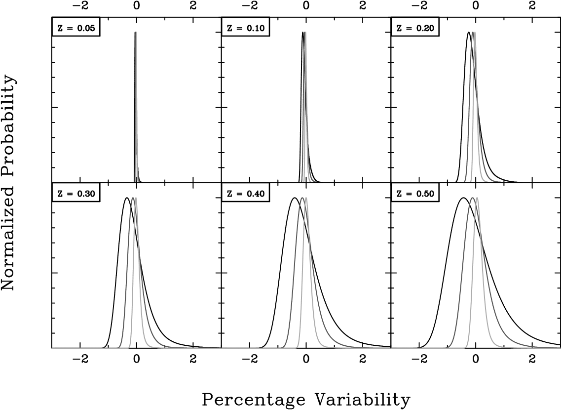
Figure 6: The distribution in total luminosity of stellar samples from $10^{5}{\rm\,L_{\odot}}$ (broadest - dark grey) to $10^{7}{\rm\,L_{\odot}}$ (narrowest - light grey), defined by the luminosity function in the text. At very low redshifts, the low microlensing optical depth induces only negligible variability, while by a redshift of $z=0.5$, fluctuations of order a percent are induced. The integrated properties of these distributions are given in Table 1.

Figure 7: The variability time scale for a $10^{-3}M_{\odot}$ microlensing mass with a relative transverse velocity of 1000${\rm\,km\,s^{-1}}$, for sources at $z=$ 0.1, 0.2, 0.3, 0.4 & 0.5 .

Figure 8: The cumulative magnification probabilities for sources at $z=$ 0.05, 0.1, 0.2, 0.3, 0.4 & 0.5 .

Figure 9: The optical depth out to $z=0.5$ in several cosmologies. At the low redshifts considered, the introduction of a cosmological constant has only a small influence on the optical depths.

Table 1:

			10%	30%	50%	70%	90%
	$10^{5}{\rm L_{\odot}}$		$\pm$0.010	$\pm$0.027	$\pm$0.040	$\pm$0.052	$\pm$0.065
z=0.05	$10^{6}{\rm L_{\odot}}$		$\pm$0.004	$\pm$0.013	$\pm$0.021	$\pm$0.029	$\pm$0.041
	$10^{7}{\rm L_{\odot}}$		$\pm$0.002	$\pm$0.005	$\pm$0.010	$\pm$0.014	$\pm$0.021
	$10^{5}{\rm L_{\odot}}$		$\pm$0.021	$\pm$0.063	$\pm$0.101	$\pm$0.138	$\pm$0.186
z=0.10	$10^{6}{\rm L_{\odot}}$		$\pm$0.010	$\pm$0.031	$\pm$0.051	$\pm$0.075	$\pm$0.108
	$10^{7}{\rm L_{\odot}}$		$\pm$0.003	$\pm$0.013	$\pm$0.022	$\pm$0.033	$\pm$0.052
	$10^{5}{\rm L_{\odot}}$		$\pm$0.047	$\pm$0.139	$\pm$0.235	$\pm$0.335	$\pm$0.480
z=0.20	$10^{6}{\rm L_{\odot}}$		$\pm$0.022	$\pm$0.070	$\pm$0.122	$\pm$0.177	$\pm$0.266
	$10^{7}{\rm L_{\odot}}$		$\pm$0.009	$\pm$0.027	$\pm$0.046	$\pm$0.071	$\pm$0.116
	$10^{5}{\rm L_{\odot}}$		$\pm$0.072	$\pm$0.215	$\pm$0.365	$\pm$0.530	$\pm$0.786
z=0.30	$10^{6}{\rm L_{\odot}}$		$\pm$0.036	$\pm$0.104	$\pm$0.187	$\pm$0.277	$\pm$0.427
	$10^{7}{\rm L_{\odot}}$		$\pm$0.010	$\pm$0.040	$\pm$0.070	$\pm$0.108	$\pm$0.175
	$10^{5}{\rm L_{\odot}}$		$\pm$0.092	$\pm$0.285	$\pm$0.490	$\pm$0.720	$\pm$1.094
z=0.40	$10^{6}{\rm L_{\odot}}$		$\pm$0.047	$\pm$0.143	$\pm$0.252	$\pm$0.373	$\pm$0.578
	$10^{7}{\rm L_{\odot}}$		$\pm$0.016	$\pm$0.052	$\pm$0.088	$\pm$0.137	$\pm$0.233
	$10^{5}{\rm L_{\odot}}$		$\pm$0.112	$\pm$0.352	$\pm$0.608	$\pm$0.899	$\pm$1.377
z=0.50	$10^{6}{\rm L_{\odot}}$		$\pm$0.049	$\pm$0.168	$\pm$0.305	$\pm$0.459	$\pm$0.715
	$10^{7}{\rm L_{\odot}}$		$\pm$0.005	$\pm$0.057	$\pm$0.108	$\pm$0.159	$\pm$0.279

Note. — The integrated properties of the probability distributions given in Figure 6. The columns presents the range over which 10, 30, 50, 70 & 90% of the magnifications are found, relative to the mean value (i.e for a $10^{6}{\rm L_{\odot}}$ population at z=0.40, 50% of all magnifications lie within $\pm 0.252\%$ of the mean value).

References

- Alcock et al. (1993) Alcock, C. et al. 1993, Nature, 365, 621
- Alcock et al. (1999) Alcock, C., et al. 1999, ApJ, 521, 602
- Alexander (1995) Alexander, T. 1995, MNRAS, 274, 909
- Baganoff & Malkan (1995) Baganoff, F. K. & Malkan, M. A. 1995, ApJ, 444, L13
- Canizares (1982) Canizares, C. R. 1982, ApJ, 263, 508
- Chang & Refsdal (1979) Chang, K. and Refsdal, S. 1979, Nature, 282, 561.
- Chang (1984) Chang, K. 1984, A&A, 130, 157
- Crotts (1992) Crotts, A. P. S. 1992, ApJ, 399, L43
- Crotts & Tomaney (1996) Crotts, A. P. S. & Tomaney, A. B. 1996, ApJ, 473, L87
- Dalcanton et al. (1994) Dalcanton, J. J., Canizares, C. R., Granados, A. , Steidel, C. C. & Stocke, J. T. 1994, ApJ, 424, 550
- Dyer & Roeder (1972) Dyer, C. C. & Roeder, R. C. 1972, ApJ, 174, L115
- Dyer & Roeder (1973) Dyer, C. C. & Roeder, R. C. 1973, ApJ, 180, L31
- Dyer & Roeder (1974) Dyer, C. C. & Roeder, R. C. 1974, ApJ, 189, 167
- Fukuda et al. (1998) Fukuda, Y. et al. 1998, Phys. Rev. Lett., 81(8), 1562
- Garnavich, et al. (1998) Garnavich, P. M., et al. 1998, ApJ, 509, 74
- Gould (1995) Gould, A. 1995, ApJ, 455, 44
- Gould (1996) Gould, A. 1996, ApJ, 470, 201
- Gwyn & Hartwick (1996) Gwyn, S. D. J. & Hartwick, F. D. A. 1996, ApJ, 468, L77
- Hawkins (1993) Hawkins, M. R. S. 1993, Nature, 366, 242
- Hawkins (1996) Hawkins, M. R. S. 1996, MNRAS, 278, 787
- Hawkins (1998) Hawkins, M. R. S. 1998, “Hunting Down the Universe”, Perseus Books
- Hawkins & Taylor (1997) Hawkins, M. R. S. & Taylor, A. N. 1997, ApJ, 482, L5
- Jahreis & Wielen (1997) Jahreis, H. & Wielen, R. 1997, in: B. Battrick, M.A.C. Perryman and P.L. Bernacca (eds.): HIPPARCOS ’97. Presentation of the Hipparcos and Tycho catalogues and first astrophysical results of the Hipparcos space astrometry mission, Venice, Italy, 13-16 May(1997; ESA SP-402, Noordwijk, p.675-680
- Kofman, Kaiser, Lee & Babul (1997) Kofman, L. , Kaiser, N. , Lee, M. H. & Babul, A. 1997, ApJ, 489, 508
- Lauer, et al. (1998) Lauer, T. R., Tonry, J. L., Postman, M. , Ajhar, E. A. & Holtzman, J. A. 1998, ApJ, 499, 577
- Lee, Babul, Kofman & Kaiser (1997) Lee, M. H. , Babul, A. , Kofman, L. & Kaiser, N. 1997, ApJ, 489, 522
- Lewis & Irwin (1995) Lewis, G. F. & Irwin, M. J. 1995, MNRAS, 276, 103
- Lewis, Miralda-Escude, Richardson & Wambsganss (1993) Lewis, G. F., Miralda-Escude, J. , Richardson, D. C. & Wambsganss, J. 1993, MNRAS, 261, 647
- Linder (1988) Linder, E. V. 1988, A&A, 206, 190
- Linder, Wagoner & Schneider (1988) Linder, E. V., Wagoner, R. V. & Schneider, P. 1988, ApJ, 324, 786
- Melchior et al. (1999) Melchior, A. -L. et al. 1999, A&AS, 134, 377
- Metcalf & Silk (1999) Metcalf, R. B. & Silk, J. 1999, ApJ, 519, L1
- Paczynski (1986) Paczynski, B. 1986, ApJ, 304, 1
- Paczynski & Wambsganss (1989) Paczynski, B. & Wambsganss, J. 1989, ApJ, 337, 581
- Peacock (1986) Peacock, J. A. 1986, MNRAS, 223, 113
- Rauch (1991) Rauch, K. P. 1991, ApJ, 374, 83
- Rauch (1991a) Rauch, K. P. 1991a, ApJ, 383, 466
- Rauch, Mao, Wambsganss & Paczynski (1992) Rauch, K. P., Mao, S. , Wambsganss, J. & Paczynski, B. 1992, ApJ, 386, 30
- Schneider (1993) Schneider, P. 1993, A&A, 279, 1
- Schneider, Ehlers & Falco (1992) Schneider, P., Ehlers, J. & Falco, E. E. 1992, Gravitational Lenses, XIV, Springer-Verlag Berlin Heidelberg New York.
- Schneider & Wagoner (1987) Schneider, P. & Wagoner, R. V. 1987, ApJ, 314, 154
- Schneider & Weiss (1988) Schneider, P. & Weiss, A. 1988, ApJ, 327, 526
- Schneider & Weiss (1988a) Schneider, P. & Weiss, A. 1988a, ApJ, 330, 1
- Thomsen, Baum, Hammergren & Worthey (1997) Thomsen, B. , Baum, W. A., Hammergren, M. & Worthey, G. 1997, ApJ, 483, L37
- Tomaney & Crotts (1996) Tomaney, A. B. & Crotts, A. P. S. 1996, AJ, 112, 2872
- Tonry & Schneider (1988) Tonry, J. & Schneider, D. P. 1988, AJ, 96, 807
- Wambsganss (1992) Wambsganss, J. 1992, ApJ, 386, 19
- Wambsganss, Paczynski & Katz (1990) Wambsganss, J., Paczynski, B. & Katz, N. 1990, ApJ, 352, 407
- Weinberg (1976) Weinberg, S. 1976, ApJ, 208, L1