Cosmological constraints from the correlation function of galaxy clusters

Abstract

I compare various semi-analytic models for the bias of dark matter halos with halo clustering properties observed in recent numerical simulations. The best fitting model is one based on the collapse of ellipsoidal perturbations proposed by Sheth, Mo & Tormen (1999), which fits the halo correlation length to better than 8 per cent accuracy. Using this model, I confirm that the correlation length of clusters of a given separation depends primarily on the shape and amplitude of mass fluctuations in the universe, and is almost independent of other cosmological parameters. Current observational uncertainties make it difficult to draw robust conclusions, but for illustrative purposes I discuss the constraints on the mass power spectrum which are implied by recent analyses of the APM cluster sample. I also discuss the prospects for improving these constraints using future surveys such as the Sloan Digital Sky Survey. Finally, I show how these constraints can be combined with observations of the cluster number abundance to place strong limits on the matter density of the universe.

1 Introduction

Recent years have seen dramatic increases in the size of the largest cosmological N-body simulations, with giga-particle runs now able to track the non-linear gravitational evolution of a significant fraction of the observable universe (Colberg et al. 1998). Correspondingly, it is becoming possible to make more and more detailed predictions for the non-linear properties of dark matter in any cosmological model, with convergent results being obtained for such features as the profiles and correlation functions of dark matter halos (Moore et al. 1999). In spite of these advances, the one great challenge remaining for the simulators is to realistically track the evolution of cosmic gas through its complex cycles of star-formation and feedback.

Given the current state of the art for cosmological simulations, rich clusters of galaxies provide one of the most powerful tools with which to make detailed tests of cosmology. Firstly, cluster potential wells are so deep that their formation and evolution is largely unaffected by the uncertain history of the cosmic gas, making dissipationless N-body simulations an ideal place in which to study their properties. Second, clusters correspond to rare peaks in the primordial density field, so their statistics are extremely sensitive to detailed features of the cosmology.

In this paper, I will show that a simple model proposed by Sheth, Mo & Tormen (1999) can give an extremely good fit to the correlation function of massive halos observed in recent state of the art numerical simulations. Using this model I will compare the predictions of a range of cosmological models with observations of the cluster correlation length. In particular, I will show that correlation length observations place strong constraints on the power spectrum of mass fluctuations in the universe, constraints that are almost independent of other cosmological parameters. In section 2 I describe the Sheth, Mo & Tormen model for the cluster correlation length, together with a similar semi-analytic model due to Mo & White (1996), and other bias models discussed in the literature. In section 3 I compare the predictions of these models with recent numerical simulations, and in section 4 I show the constraints which can be derived when the models are compared with observations. In section 5 I discuss the relationship of this work to previous studies, and draw my conclusions.

2 Models for the correlation length

I describe four semi-analytic models which make predictions for the amplitude of halo correlations, one due to Mo & White (1996 – hereafter MW), one due to Sheth, Mo & Tormen (1999 – hereafter SMT), one due to Sheth and Tormen (1999 – hereafter ST), and one based on a model by Lee & Shandarin (1998 – hereafter LS) and extended in ST. The input parameters for these models are the power spectrum of matter fluctuations $P(k)$ (extrapolated using linear gravity to today) and the background cosmology of the universe (specified here in terms of $\Omega_{\rm m}$ and $\Omega_{\Lambda}$, the contributions of matter and a cosmological constant to the critical density today). I will compare the predictions of these models with observations of the halo correlation length $r_{0}(d)$, defined such that $\xi(r_{0})=1$ where $\xi(r)$ is the halo correlation function. Also, $d$ is the mean halo separation for the halo sample in question, and the sample is chosen to contain only those halos with “richness” greater than some value. In this context I use “richness” (${\cal R}$) to denote any parameter which correlates with halo mass (typical examples for clusters are galaxy number counts and X-ray luminosity). I will assume that the parameter $R$ can be monotonically transformed into an “inferred mass” ${\cal M}=f({\cal R})$ which is correlated with the true mass with known conditional probability $p({\cal M}|M)$.

For each model, the procedure for computing the correlation length for a sample of halos with mean separation $d$ is as follows.

• First, compute the inferred mass threshold ${\cal M}$, such that the mean separation of halos with inferred mass greater than ${\cal M}$ is equal to $d$. That is, find ${\cal M}$ satisfying

  $$N^{\rm I}_{X}({\cal M})=d^{-3}$$ (1)

  where $N^{\rm I}_{\rm X}({\cal M})$ is the number density of halos with inferred (as denoted by the superscript I) mass greater than ${\cal M}$ for model X, and X denotes the semi-analytic formalism being used (either MW, SMT, ST or LS). Now,

  $$N^{\rm I}_{\rm X}({\cal M})=\int_{\cal M}^{\infty}n^{\rm I}_{X}({\cal M})d{\cal M}$$ (2)

  where $n^{\rm I}_{X}({\cal M})d{\cal M}$ is the number density of halos with inferred masses between ${\cal M}$ and ${\cal M}+d{\cal M}$, and

  $$n^{\rm I}_{X}({\cal M})=\int dMp({\cal M}|M)n_{X}(M)$$ (3)

  with

  $$n_{X}(M)=-\nu f_{X}(\nu)\frac{\bar{\rho}}{M}\frac{d\sigma(M)/dM}{\sigma(M)}$$ (4)

  being the number density of halos with true mass between $M$ and $M+dM$. Here $\nu=\delta_{c}/\sigma(M)$, $\sigma(M)$ is the rms linear fluctuation in a sphere containing an average mass $M$, $\bar{\rho}$ is the background density of the universe, and $\delta_{c}$ is the critical overdensity for collapse as computed in the spherical collapse model – see Kitayama & Suto (1996) for fits to the weak cosmological dependence. The quantity $\sigma(M)$ can be straightforwardly calculated at any redshift knowing $P(k)$ and the background cosmology. The function $f_{X}$ is given by

  $$f_{\rm MW}(\nu)=\sqrt{\frac{2}{\pi}}\exp\left(-\frac{\nu^{2}}{2}\right)$$ (5)

  for the MW model, by

  $$f_{\rm SMT}(\nu)=f_{\rm ST}(\nu)=A\left(1+\frac{1}{a^{q}\nu^{2q}}\right)\sqrt{\frac{2}{\pi}}\exp\left(-\frac{a\nu^{2}}{2}\right)$$ (6)

  for the SMT and ST models, with $A\simeq 0.3222$, $q=0.3$, and $a=0.707$, and by equation A1 of ST for the LS model.

• Calculate the effective bias parameter $b^{X}_{>{\cal M}}$ for halos with an inferred mass greater than ${\cal M}$, satisfying

  $$b^{X}_{>{\cal M}}=\frac{1}{N^{I}_{X}({\cal M})}\int_{\cal M}^{\infty}b^{I}_{X}({\cal M})n^{I}_{X}({\cal M})dM$$ (7)

  where

  $$b^{I}_{X}({\cal M})=\frac{\int dMp({\cal M}|M)f_{z}(b_{X}(M))b_{X}(M)n(M)}{\int dMp({\cal M}|M)n(M)}$$ (8)

  and $b_{X}(M)$ is the bias parameter for halos with true mass $M$, given by

  $$b_{\rm MW}=1+\frac{1}{\delta_{c}}(\nu^{2}-1)$$ (9)

  for the MW model, by

  $$b_{\rm SMT}= 1+\frac{1}{\sqrt{a}\delta_{c}} \left[a^{5/2}\nu^{2}+\sqrt{a}b(a\nu)^{2(1-c)}\right.$$ (11)

  $$\left.-\frac{(a\nu)^{2c}}{(a\nu)^{2c}+b(1-c)(1-c/2)}\right]$$

  for the SMT model with $a=0.707$, $b=0.5$ and $c=0.6$, by

  $$b_{\rm ST} = 1+\frac{1}{\delta_{c}}\left[(a\nu^{2}-1)+\frac{2q}{1+\left(a\nu^{2}\right)^{q}}\right]$$ (12)

  for the ST model with $a$ and $q$ given above, and by equation A3 of ST for the LS model. Lastly, $f_{z}$ is an optional factor which may be included to account for the effect of redshift space distortion if the prediction is to be compared with observations in redshift space. Following Kaiser (1987) $f_{z}$ is given by

  $$f_{z}(b)=1+2\beta/3+\beta^{2}/5$$ (13)

  where $\beta=\Omega_{m}^{0.6}/b$.

• Solve for the correlation length $r_{0}$ satisfying $(b^{X}_{>{\cal M}})^{2}\xi_{\rm NL}(r_{0})=0$, where $\xi_{\rm NL}(r)$ is the non-linear mass correlation function, given by the Fourier transform of the non-linear power spectrum $P_{\rm NL}(k_{\rm NL})$. The non linear power spectrum is computed using the method described by Peacock & Dodds (1996) using the linear power spectrum $P(k)$ as input. For comparison, we also compute $r_{0}$ using the linear correlation function, that is we solve for $r_{0}$ satisfying $(b^{X}_{>{\cal M}})^{2}\xi_{\rm L}(r_{0})=1$, where $\xi_{\rm L}(r)$ is the Fourier transform of the linear power spectrum $P(k)$. As we will see in section 3, use of the non-linear correlation function gives a better fit for all the models. Unless otherwise specified, all correlation lengths have been computed using the non-linear correlation function.

3 Comparison with simulations

The models just described make predictions for the halo two-point correlation function on any length scale $r$. Since the shape of the halo correlation function is not well constrained by current observations, most authors have focused just on the amplitude, quantified in terms of the correlation length $r_{0}$. I now compare the predictions of each of the models for $r_{0}$ with the values observed in large collisionless N-body simulations (comparison between models and simulations for the full halo correlation function is beyond the scope of the current paper, but deserves future investigation). The simulations have been carried out by Colberg et al. (1998 – hereafter C98) and Governato et al. (1999 – hereafter G99). For each simulation the power spectrum has been taken to have a CDM form (Bardeen et al. 1986, eq. G3) parameterized by a shape parameter $\Gamma$ (where $\Gamma\simeq\Omega h$, and $h$ is the Hubble constant in units of 100 kms^-1Mpc^-1) and normalization $\sigma_{8}$, where $\sigma_{8}$ is the rms fluctuation in an $8h^{-1}$Mpc sphere. The power spectrum parameters for each simulation are summarized in Table 1, together with the box length $L$, particle number $N_{p}$ and background cosmology. Fig. 1 compares the $r_{0}-d$ relation observed in the simulations (data points) with that predicted by the MW (dotted lines) and SMT (solid lines) formalisms. In computing these predictions, I use $p({\cal M}|M)=\delta({\cal M}-M)$ where $\delta$ denotes the Dirac delta function, since in this case the richness property by which the halos are ranked is just the true mass.

Figure 1: Correlation length versus halo separation as observed in numerical simulations (datapoints) together with the predictions of the SMT (solid curves) and MW (dotted curves) models. The SMT predictions agree very closely with the results of the simulations, while the MW predictions are typically 25 per cent too high.

Clearly the SMT model gives much better agreement with the cluster correlation length as observed in the simulations. I quantify the goodness of fit by defining an rms error $E$ via

$$E^{2}=\frac{1}{N}\sum_{\rm i=1}^{N}\left(\frac{r^{\rm i}_{0}-r^{\rm X}_{0}(d^{i})}{r^{\rm X}_{0}(d^{i})}\right)^{2}$$ (14)

where the sum $i$ runs over all datapoints ($d^{i}$,$r^{i}_{0}$) under consideration, and $r^{\rm X}_{0}(d)$ denotes the correlation length prediction for model X at separation $d$. For the combined datapoints from all four simulations, the SMT model gives $E=0.08$, while errors for the MW model are much larger, with $E=0.22$. The goodness of fit for each of the models is given in Tab 2. The left column shows results using the non-linear correlation function to compute $r_{0}$, while the right column shows results using the linear correlation function. Use of the non-linear correlation function improves the fit in each case.

Model	Source	$\Omega_{\rm m}$	$\Omega_{\Lambda}$	$\sigma_{8}$	$\Gamma$	$N_{p}$	$L/(h^{-1}\rm{Mpc})$
SCDM07	G99	1.0	0.0	0.7	0.5	$47\times 10^{6}$	$500$
O3CDM	G99	0.3	0.0	1.0	0.225	$47\times 10^{6}$	$500$
$\tau$CDM	C98	1.0	0.0	0.6	0.21	$10^{9}$	$2000$
LCDM	C98	0.3	0.7	0.9	0.21	$10^{9}$	$3000$

Table 1: Summary of parameters for each of the simulations discussed in section 3.

I conclude from this analysis that the SMT model gives a good fit (typical errors less than 8 per cent) to the halo correlation length arising from a full treatment of the non-linear gravitational evolution. The MW model does worst of all the models considered, with typical errors of order 25 per cent. In particular, the MW model systematically overestimates the halo correlation length for fixed separation $d$, a result also found in C98. It is worth noting that the discrepancy between the MW model and the simulations is much larger than might be inferred from previous studies. For instance, Mo, Jing & White (1996 - hereafter MJW) and Jing (1999) suggest that the MW formula agrees at better than the five per cent level with the rare halo bias observed in their simulations. Closer examination of the rarest mass datapoints in Fig. 3 of Jing (1999) illustrate that the error is actually much larger. Figs. 7 and 8 of Governato et al. also imply extremely good agreement between the MW formula and correlation lengths observed in their simulations. In fact, the MW prediction has been computed incorrectly in these figures, and the true agreement is much worse (as illustrated in Fig. 1 of this paper). A final source of confusion as to the accuracy of the MW formula is that the curves showing the MW prediction in Fig. 8 of MJW have also been computed incorrectly, with the correct values for the correlation length being up to 25 per cent higher in some places. To summarize, there is clear evidence that the MW formula significantly overestimates the expected bias of the rarest halos, while the SMT model gives extremely good agreement.

Model	$E$–$(\xi_{\rm NL})$	$E$– $(\xi_{\rm L})$
MW	0.22	0.24
SMT	0.08	0.10
ST	0.11	0.12
LS	0.11	0.14

Table 2: Goodness of fit for each of the bias models discussed in section 2. The fit parameter $E$ is defined in section 3. The first and second columns give the fit obtained using the non-linear and linear correlation function respectively.

4 Comparison with data

I now make use of the SMT model to compare the predictions of a range of cosmologies with observational data. Fig. 2 shows the $r_{0}-d$ relation for the APM cluster survey, as analyzed by Croft et al. (1997 - hereafter C97) and Lee & Park (1998 - hereafter LP98). Although this is only a small fraction of currently available data on the cluster correlation length, it suffices to illustrate the wide degree of systematic uncertainty which exists in present observations – even two analyses of the same dataset give results that differ by considerable factors, and the situation is even less clear when results from Abell (see for instance Bahcall & Cen 1992) and X-ray (see LP99 for a detailed discussion) cluster samples are included. Although present day uncertainties are large, errors in $r_{0}$ will be greatly reduced by future surveys. The Sloan Digital Sky Survey (SDSS, see project book at http://www.astro.princeton.edu/PBOOK/welcome.htm for detailed specifications) is expected to identify roughly 1000 nearby clusters in its spectroscopic galaxy redshift survey, and even more in its photometric survey. The inclusion of redshift information in the cluster identification procedure will greatly reduce systematic uncertainties in $r_{0}$, and statistical uncertainties will be reduced by approximately 50 per cent by the increased sample size. In order to illustrate the type of results we can hope for, I will carry out the bulk of my analysis using just the C97 data. This data is at least self-consistent, and 2$\sigma$ confidence limits for the SDSS survey should be similar in size to 1$\sigma$ confidence limits from the C97 analysis.

Figure 2: Cluster correlation length versus halo separation as inferred by Croft et al. (1997 - solid squares) and Lee and Park (1999 - open triangles) from an analysis of the APM cluster sample. The solid line shows the SMT prediction for a model with $\Omega_{m}=0.3$, $\Gamma=0.17$ and $\sigma_{8}=1.0$.

I compute confidence limits for various models as follows: Each model gives a specific prediction for the for the $r_{0}-d$ relation, given which the likelihood of observing a particular dataset is (up to a constant of proportionality)

$${\cal L}\propto e^{-\chi^{2}/2}$$ (15)

where

$$\chi^{2}=\sum_{\rm i}\frac{\left(r^{\rm i}_{0}-r^{\rm X}_{0}(d^{i})\right)^{2}}{\sigma^{2}_{i}+\left(Er^{\rm X}_{0}(d^{i})\right)^{2}}.$$ (16)

Here the sum $i$ runs over all datapoints ($d_{i}$,$r^{i}_{0}$) with standard deviation $\sigma_{i}$, $E$ is the fractional uncertainty in the predictions of the model (which following the discussion in section 3 is taken to be $E=0.08$) and the term $\left(Er^{\rm X}_{0}(d^{i})\right)^{2}$ is added in quadrature to the denominator to account for systematic uncertainties in the model. Given a set of model parameters and prior distributions for those parameters, I calculate $1\sigma$ and $2\sigma$ confidence limits by computing the likelihood threshold above which the integrated likelihood accounts for 69 and 95 per cent respectively of the total probability. Finally, all model predictions are computed at the median redshift of each sample, which I take to be $z=0.08$, although the precise value used has little effect on the results.

Fig. 3 shows confidence limits in the $\Gamma-\sigma_{8}$ plane derived from the observations shown in Fig. 2. Given values for $\sigma_{8}$ and $\Gamma$, each model is fully specified once we know $\Omega_{\rm m}$ and the conditional probability distribution relating the “inferred” mass for the cluster observations in question to the true cluster mass. The shaded area labeled “Croft” shows 1$\sigma$ (dark region) and 2$\sigma$ (light region) confidence limits derived using the SMT model and the C97 data, in an $\Omega_{m}=0.3$ background cosmology with zero scatter between inferred and true cluster mass (use of an open $\Omega_{\rm m}=0.3$ cosmology makes virtually no difference to the results).

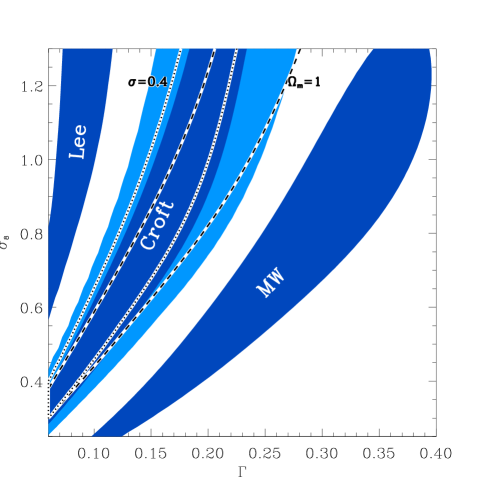
Figure 3: Confidence limits in the $\Gamma-\sigma_{8}$ plane derived from cluster correlation length data. The shaded area labeled “Croft” shows 1$\sigma$ (dark band) and 2$\sigma$ (light band) limits derived from the fiducial analysis utilizing the Croft data and assuming the SMT model for cluster correlations, in an $\Omega_{m}=0.3$, $\Omega_{\Lambda}=0.7$ cosmology with zero scatter between true and inferred cluster mass. Each of the other four bands show the results of changing one factor in the fiducial analysis; using the Lee & Park (1999) analysis of the APM clusters (shaded area labeled Lee), using the MW correlation length formula (shaded area labeled MW), using a flat $\Omega_{m}=1.0$ cosmology (area delineated by long-dashed lines), and finally using a 50 per cent scatter between true and inferred cluster mass (area delineated by short-dashed lines).

Four other confidence regions are also shown in this figure, each one the result of changing one aspect of the first analysis. First, the shaded area labeled “MW” gives the $1\sigma$ confidence region which results from using the MW model rather than the SMT model. The limits in this case are quite different, and given the poor performance of the MW model when compared to simulations, should be disregarded. Second, the shaded region labeled “Lee” shows the 1$\sigma$ limits resulting from using the LP99 data (with its higher values for $r_{0}$) rather than the C98 data. The LP99 data favours dramatically lower values of $\Gamma$ for a given value of $\sigma_{8}$, and since the majority of alternative datasets (see LP99 for a detailed discussion) also prefer higher values of $r_{0}$, the high $\Gamma$ region to the right of the “Croft” confidence limits is likely to be excluded by all current observations. Thirdly, the long-dash lines delineate the 1$\sigma$ confidence region resulting from an analysis identical to the “Croft” analysis except for the choice of a flat $\Omega_{\rm m}=1$ cosmology. Increasing $\Omega_{\rm m}$ slightly increases the amplification of clustering by redshift space distortion, and slightly reduces the growth factor at the median redshift of the sample. Both of these effects are small, and the resulting confidence region is very similar to the $1\sigma$ limits resulting from the $\Omega_{\rm m}=0.3$ analysis. Lastly, the short dashed lines delineate 1$\sigma$ confidence regions obtained when a significant scatter is introduced between the inferred and true cluster masses. In particular, $p({\cal M}|M)$ is modeled as a log-normal distribution with a natural logarithmic standard deviation $\sigma=0.4$. This value of $\sigma$ corresponds to roughly a 50 per cent scatter in the inferred mass for a given true mass. Even for such a large scatter, the 1$\sigma$ confidence region is virtually unchanged, demonstrating that robust constraints can be obtained even if clusters of a given mass have a wide distribution of “richness” values - the only requirement is that there is some monotonic transformation which loosely correlates the richness (for instance, X-ray luminosity or galaxy counts) with the true mass.

Fig. 3 demonstrates that observations of the cluster correlation length place constraints on the amplitude & shape of the matter power spectrum in the universe which are almost independent of cosmology. As one final point, I illustrate the type of cosmological constraints which can be obtained when these limits are combined with independent observations of the mass power spectrum. Fig. 4 shows confidence limits in the $\Omega_{\rm m}-\sigma_{8}$ plane from a combination of cluster correlation length data and cluster number abundance data. The dark and light hashed regions show 1$\sigma$ and 2$\sigma$ confidence bands derived from the local cluster temperature function by Eke, Cole & Frenk (ECF - 1996). The other confidence bands show 1$\sigma$ and 2$\sigma$ limits derived from the C97 data, under three different assumptions about the value of $\Gamma$. The solid lines show constraints for the case of a CDM cosmology with $\Gamma=\Omega_{\rm m}h\exp(-\Omega_{\rm B}(1+\sqrt{2h}/\Omega_{\rm m}))$ with $h=0.65$, and $\Omega_{\rm B}=0.04$ (for conciseness, this region is simply labeled by “$\Gamma=\Omega_{\rm m}h$”). Increases (decreases) in the value of $h$ just shift the confidence region to lower (higher) values of $\Omega_{\rm m}$ by the same factor. The shaded bands show confidence limits for the choices $\Gamma=0.23$ (which provides a good fit to the power spectrum of APM galaxies - see Viana & Liddle 1996) and $\Gamma=0.1$. For $\Gamma=0.1$ the combined ECF and C97 constraints are consistent with the case $\Omega_{\rm m}=1$, while the other choices for $\Gamma$ each require $\Omega_{\rm m}<0.35$ for consistency between the datasets at the 2$\sigma$ level. If the LP99 data was used instead of C97, even lower values of $\Omega_{\rm m}$ would be preferred.

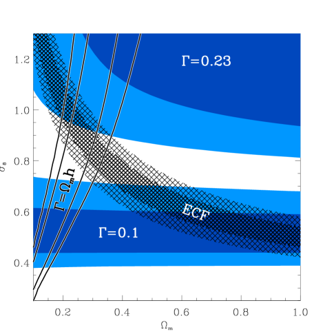
Figure 4: Confidence limits in the $\Omega_{\rm m}-\sigma_{8}$ plane derived from cluster correlation length data and cluster abundance data. The hashed area labeled “ECF” shows 1$\sigma$ (dark band) and 2$\sigma$ (light band) limits from the cluster abundance analysis of Eke, Cole & Frenk (1996). Each of the other three bands shows correlation length constraints from the C97 data, under three different assumptions about the value of $\Gamma$, as labeled. For the $\Gamma=\Omega_{\rm m}h$ case I take h=0.65.

5 Conclusion

I have shown that the halo correlation length measured in recent numerical simulations can be well fit (to better than 8 per cent accuracy) by a semi-analytic model based on the collapse of ellipsoidal perturbations due to Sheth, Mo & Tormen (1999). A similar analytic model due to Mo & White (1996) on the other hand gives a poorer fit to the simulations (roughly 25 per cent accuracy). Applying the SMT result to present data, I have shown that correlation length observations place strong, almost cosmology independent constraints on the shape and amplitude of the matter power spectrum in the universe. By far the greatest source of uncertainty is systematic discrepancies between current datasets, but if the cluster correlation length is at least as high as is implied by the APM survey, then an interesting region of power spectrum parameter space (everything to the right of the “Croft” region in Fig. 3) can be excluded. Future surveys, including the Sloan Digital Sky Survey, should greatly reduce the observational uncertainties, with 2$\sigma$ confidence limits from SDSS being as tight as the 1$\sigma$ limits shown for the C97 data in Fig. 3. One particularly interesting result is that the analysis is almost unaffected when a significant scatter (up to 50 per cent) is introduced between true cluster mass and the richness property by which clusters are ranked. Such a scatter is inevitable in any cluster survey, so it is extremely useful to know that even an effect this large does not influence the results. Finally, I have shown how the correlation length can be combined with other cluster observations to place limits on the matter density of the universe.

A number of previous studies have discussed constraints from the cluster correlation length. Bahcall & Cen (1992) and Croft & Efstathiou (1994) carried out numerical simulations showing that cluster correlation length was a strong discriminator amoung models, and obtained results which are consistent with those discussed in this paper. Mo, Jing & White (1996) and later Robinson, Gawiser & Silk (1998) made use of the MW formalism to compare models and observations for a wider range of parameters, and owing to the inaccuracy of the MW model, their results are not consistent with those found here (the inconsistency of the MW model is actually larger than is apparent in MJW due to an error in Fig. 8 of that paper). The work described here improves on previous studies by utilizing a formula which accurately fits the most recent numerical simulations, and which can be used to compute predictions for a large range of model parameters very quickly.

Lastly, it should be noted that the analysis discussed here assumes that the primordial fluctuations in the universe are Gaussian. Non-gaussianity also influences the value of the cluster correlation length, and a number of authors, including Robinson, Gawiser & Silk (1998) and Koyama, Soda & Taruya (1999) have attempted to exploit this fact to use cluster observations to place constraints on primordial non-gaussianity. Both these works have modeled the correlation function for non-gaussian models using an extension of the MW formalism, and therefore their conclusions should be modified in the light the results discussed here, which show that MW does not accurately predict the halo correlation function even for Gaussian models.

To summarize, cluster correlation length observations place strong cosmology independent constraints on the matter power spectrum in the universe, constraints which future surveys such as SDSS will allow us to fully exploit.

6 acknowledgements

I would like to thank Marc Davis, Eric Gawiser and Joseph Silk for helpful and stimulating discussions. I would also like to thank Fabio Governato and H. J. Mo for their swift answers to my questions, and Pedro Ferreira for reading a draft of the manuscript. This work has been supported in part by grants from the NSF, including grant 9617168.

References

- [1]
- [2] Bahcall N. A, Cen R., 1992, ApJ, 398, L81
- [3] Colberg J. M., White S. D. M., MacFarland T. J., Jenkins A., Frenk C. S., Pearce F. R., Evrard A. E., Couchman H. M. P., Efstathiou G., Peacock J. A., Thomas P. A. 1998, in proceedings of The 14th IAP Colloquium: Wide Field Surveys in Cosmology, held in Paris, 1998 May 26-30, eds. S.Colombi, Y.Mellier (C98)
- [4] Croft, R. A. C., Dalton, G. B., Efstathiou, G., Sutherland, W. J., & Maddox, S. J. 1997, astro-ph/9701040
- [5] Croft, R. A. C., Efstathiou, G., 1994, MNRAS, 267, 390
- [6] Eke V. R., Cole S., Frenk C. S., 1996, MNRAS, 282, 263
- [7] Governato F., Babul A., Quinn T., Tozzi P., Baugh C. M., Katz M., Lake G., 1999, MNRAS, 307, 949
- [8] Kaiser N., 1987, MNRAS, 227, 1
- [9] Kitayama T., Suto, Y., 1996, ApJ, 469, 480
- [10] Koyama K., Soda J., Taruya A., 1999, astro-ph/9903027
- [11] Lee J., Shandarin, S. F. 1998, ApJ, 500, 14
- [12] Lee S., Park C., 1999, astro-ph/9909008
- [13] Mo H. J., Jing Y. P., White S. D. M., 1996, MNRAS, 284, 189
- [14] Mo H. J., White S. D. M., 1996, MNRAS, 282, 347
- [15] Moore B., Ghigna S., Governato F., Lake G., Quinn T., Stadel J., Tozzi P., 1999, ApJ 524, L19
- [16] Peacock J. A., Dodds J., 1996, MNRAS, 280L, 19
- [17] Robinson J., Gawiser E., Silk J., 1998, astro-ph/9805181
- [18] Sheth R. K., Mo H. J., Tormen G., 1999, astro-ph/9907024
- [19] Sheth R. K., Tormen G., 1999, MNRAS, 308, 119
- [20] Viana P. T. P., Liddle A. R., 1996, MNRAS, 281, 531