A cosmic ray observatory with full-sky coverage can exploit standard anisotropy analysis methods that do not work if part of the celestial sphere is never seen. In particular, the distribution of arrival directions can be fully characterized by a list of spherical harmonic coefficients. The dipole vector and quadrupole tensor are of special interest, but the full set of harmonic coefficients constitutes the anisotropy fingerprint that may be needed to reveal the identity of the cosmic ray sources. The angular power spectrum is a coordinate-independent synopsis of that fingerprint. The true cosmic ray anisotropy can be measured despite non-uniformity in celestial exposure, provided the observatory is not blind to any region of the sky. This paper examines quantitatively how the accuracy of anisotropy measurement depends on the number of arrival directions in a data set.

1 Introduction

The origin of the highest energy cosmic rays is a problem that has persisted for 4 decades since the pioneering measurements at Volcano Ranch [1, 2]. There is some consensus that, above the spectrum’s ankle at about $10^{18.5}$ eV, they originate outside the disk of the Galaxy. For particles of such high magnetic rigidity, sources in the Galaxy’s disk would presumably cause an obvious anisotropy in arrival directions that is not observed. Evidence for a composition changing to lighter particles at the ankle [3] strengthens this argument (particles having even greater rigidity because of lesser charge) and supports the view that cosmic rays with energies above the ankle are of extragalactic origin. The sources of those particles remain to be identified.

The observations of cosmic rays with energies above the expected GZK cutoff [4, 5] should be a powerful clue to the nature of the sources. The Fly’s Eye [6] and AGASA [7] measured air showers with energies well above the GZK threshold. Recent reports [8, 9, 10] suggest that the spectrum might continue without a strong GZK effect. These super-GZK results have posed several related, but distinguishable, puzzles:

1. How are particles produced with such prodigious energy?

2. Why do the arrival directions of those particles not point back to recognizable sources in our local part of the universe?

3. Why is the intensity of particles above $6\times 10^{19}$ eV not more strongly suppressed?

New attempts to improve the observational data include the recently commissioned High Resolution Fly’s Eye (HiRes) [11], the Pierre Auger Observatory [12], the proposed Telescope Array Project [13], and Airwatch/OWL [14] plans for future space-based detectors of atmospheric air showers. The Auger Observatory and the potential space-based detectors will have exposure to the entire sky, which will open new possibilities for anisotropy analysis. These methods will be explored here in the context of the better controlled exposure of the Auger surface arrays.

Hillas [15] pointed out years ago that there are few astrophysical sites that can produce a large enough “electrical potential” $\beta BL$ to accelerate even highly charged nuclei to $10^{20}$ eV. (Here $\beta=v/c$ is the relative velocity of moving media with magnetic field strength $B$ and size $L$. In the case of statistical acceleration, including Fermi shock acceleration, the same product $\beta BL$ governs the maximum particle rigidity even though particles do not pass through a monotonic change in electrical potential.) Puzzle #1 is exacerbated in many contexts by synchrotron radiation and/or pion photoproduction.

Puzzle #2 can be resolved by invoking stronger-than-expected extragalactic magnetic fields, but that does not readily simplify puzzle #3. The expected suppression of particles above the GZK cutoff is based on travel time (or total distance traveled) rather than the straight-line distance to the sources. Particles below the GZK threshold have been accumulating over billions of years, whereas the mean age of particles well above the threshold cannot be greater than tens of millions of years [16].

One possible inference from the lack of an observable GZK spectral break is that sub-GZK particles may not be much older than 30 million years either, in which case the GZK effect would not significantly suppress the cosmic rays above the threshold relative to those below. It is not reasonable to suppose that the sources of high energy cosmic rays turned on so recently, so the young age of sub-GZK cosmic rays would require an intergalactic mechanism for dissipating their energy. Known mechanisms (e.g. nuclear interactions, synchrotron radiation, $e^{\pm}$ production, pion photoproduction via infrared and visible background photons, etc.) do not rob energy from sub-GZK particles rapidly enough. Perhaps high energy cosmic rays are attenuated through interactions with the unknown dark matter of the universe [17].

More conventional approaches to puzzle #3 are to defeat the GZK cutoff with a very hard extragalactic spectrum (e.g. from topological defect annihilation [18]) or to evade it by invoking neutrinos [19, 20] or non-standard particles [21, 22] that are immune to the microwave background radiation. Others [23, 24] conclude that the sources must be localized to the Galaxy, but distributed in a halo large enough that galactic anisotropy has not become obvious.

The cumulative cosmic ray observations at this time are not sufficient to sort out the possibilities. AGASA and HiRes are currently building up the world’s total exposure at the highest energies. With better statistics and better measurements, the observations could soon lead to a breakthrough that identifies the sources of the highest energy cosmic rays. This same hope has been expressed for decades through the course of numerous experiments, however, and the puzzles have only become deeper mysteries. The answers may not come easily, and we should prepare the best possible analyses of the energy spectrum, particle mass distribution, and arrival directions.

Careful determinations of the energy spectrum and mass composition can be used to weed out classes of theories, but these tools are not likely to yield a clear signature for picking out a unique theory. A positive identification of the cosmic ray sources requires seeing their fingerprint in the sky. This may come in the form of arrival direction clusters [25, 26] that identify discrete sources, or it may come as a large-scale celestial pattern that characterizes a particular class of potential sources. In the worst case, we might discover that the arrival directions are isotropic and the sources still elude positive identification. In that case, observers must strive for the best possible upper limit on anisotropy.

The Auger Project’s surface arrays will provide the best search for anisotropy fingerprints. Their combined exposure function on the celestial sphere will be unambiguous because they operate continuously and are not sensitive to atmospheric variability. Continuous operation means the celestial exposure function is uniform in right ascension. By having observatories appropriately located in both the southern and northern hemispheres, the exposure does not vary strongly with declination either.

The methods described in this paper are applicable to any observatory with full-sky coverage. They are not limited to the Auger Project, although the specific Auger site locations are used in the example simulations that are reported here.

Coverage of the full sky could be achieved piecemeal by combining results from different experiments. There is serious risk of spurious results from such meta-analyses, however, unless the exposures, energy resolutions, and detector systematics are perfectly understood and correctly incorporated in the analysis. The reliable approach is to use identical detectors in both hemispheres or the same (orbiting) detector for both hemispheres.

This paper seeks to evaluate the sensitivity of a full-sky observatory to large-scale anisotropy patterns and how that sensitivity depends on the number of arrival directions in a data set. Large-angle fingerprinting will be needed if there are many contributing sources or if the flux from each single source is diffused over a large solid angle due to magnetic deflection of the charged cosmic rays. If, instead, there are point sources to be detected, then the advantage of a full-sky observatory is in mapping the entire celestial sphere with comparable sensitivity in all regions.

Full-sky coverage is crucial for large-scale anisotropy analysis. It makes it possible to do integrals over the sky, so the powerful tools of multipole moments and angular power spectra are available. With full sky coverage, cosmic ray anisotropy analysis will be similar to gamma ray burst anisotropy analysis. The numbers of events will be comparable, the direction error boxes will be comparable, the exposure non-uniformities will be comparable, and in both cases events come from all parts of the sky. All of the techniques that were employed to search for anisotropy in the BATSE data [27, 28] can be applied to a full-sky cosmic ray data set.

With a cosmic ray detector in only one hemisphere, there is a solid angle hole in the sky where the detector has zero exposure despite the Earth’s rotation. A zero-exposure hole makes it impossible to do integrals over the whole celestial sphere. No matter how many events the detector collects overall, it will never determine any multipole moment. A single-hemisphere detector can test hypotheses like, “Does the observed distribution match better what would be accepted from the clustering of radio galaxies toward the supergalactic plane or what would be accepted from an isotropic distribution?” It can also make qualified measurements like, “Assuming the anisotropy is a perfect quadrupole with axial symmetry, fit for the axis orientation that best explains the observed celestial distribution.”

The role of an observatory, however, should be to map the sky and make results available in a form which is readily usable without knowledge of the detector properties and which is independent of any theoretical hypothesis. Low-order multipole tensors (or spherical harmonic coefficients) can summarize the large-scale information. The angular power spectrum reveals if there is clumpiness on smaller scales. These results can be tabulated so that theorists can test arbitrary models quantitatively without privileged access to the data. With approximately uniform exposure, even eyeball inspection of arrival direction scatter plots can show large-scale patterns that are hidden when steep exposure gradients dominate the scatter plots.

While the role of an observatory should be to map the sky and determine the patterns without preconceived expectations, it is nevertheless worthwhile to consider what might be learned by measuring the low order multipoles or the angular power spectrum.

Monopole. There is no information about anisotropy patterns in the monopole scalar by itself. It is simply the sky integral of the cosmic ray intensity. That is information already present in the energy spectrum. A pure monopole intensity distribution is equivalent to isotropy. The strength of other multipoles relative to the monopole is a measure of anisotropy.

Dipole. A pure dipole distribution is not possible because the cosmic ray intensity cannot be negative in half of the sky. A “pure dipole deviation from isotropy” means a superposition of monopole and dipole, with the intensity everywhere $\geq 0$.

A predominantly dipole deviation from isotropy might be expected if the sources are distributed in a halo around our Galaxy, as has been suggested [23, 24]. In this case, there is a definite prediction that the dipole vector should point toward the galactic center.

An approximate dipole deviation from isotropy could be caused by a single strong source if magnetic diffusion or dispersion distributes those arrival directions over much of the sky. In general, a single source would produce higher-order moments as well.

A dipole moment is measurable in the microwave radiation due to Earth’s motion relative to the universal rest frame [29]. If we are moving relative to the cosmic ray rest frame, a dipole moment should exist also in the cosmic ray intensity (the Compton-Getting effect). At lower energies, this may occur if the sun and Earth are moving relative to the galactic magnetic field or if the cosmic rays are not at rest with respect to the galactic field. For extragalactic cosmic rays, a Compton-Getting dipole is expected if the Galaxy is moving relative to the intergalactic field or if the cosmic rays themselves are streaming in intergalactic space. In any case, the expected velocities would be small ($v/c\lower 2.15277pt\hbox{$\;\buildrel<\over{\sim}\;$}10^{-3}$), and the Compton Getting anisotropy [30] ($\frac{I_{max}-I_{min}}{I_{max}+I_{min}}=(\gamma+2)(v/c)$) should be $\lower 2.15277pt\hbox{$\;\buildrel<\over{\sim}\;$}0.005$. (Here $\gamma$ is the differential spectral index, which is roughly 3.) An anisotropy of one-half percent would require high statistics for detection (see section 3).

A larger dipole anisotropy might be produced by a cosmic ray density gradient. If the magnetic field is disorganized, the gradient produces streaming by diffusion and the Compton-Getting dipole vector is parallel to the density gradient. If there is a regular magnetic field, however, the expected dipole vector $\vec{D}$ can be perpendicular to both the gradient and the field direction, $\vec{D}\propto\vec{\nabla}\rho\times\vec{B}$. The direction of strongest intensity corresponds to the arrival direction of particles whose orbit centers are located in the direction of increased density.

Quadrupole. An equatorial excess in galactic coordinates or supergalactic coordinates would show up as a prominent quadrupole moment. A measurable quadrupole is expected in many scenarios of cosmic ray origins, and is perhaps to be regarded as the most likely result of a sensitive anisotropy search.

In general, a quadrupole tensor is characterized by 3 relative eigenvalues with associated orthogonal eigenvectors. In the case of axial symmetry, there is a single non-degenerate eigenvector that gives the symmetry axis. An axisymmetric “prolate” distribution would be hot spots at antipodal points of the sky, whereas an “oblate” distribution has the excess concentrated toward the equator that is perpendicular to the symmetry axis.

The axis of an oblate quadrupole distribution might differ from the galactic axis or the supergalactic axis if we are embedded in a magnetic field that systematically rotates the arrival directions.

The angular power spectrum. Spherical harmonic coefficients for a function on a sphere are the analogue of Fourier coefficients for a function on a plane. Variations on an angular scale of $\theta$ radians contribute amplitude in the $\ell=1/\theta$ modes just as variations of a plane function on a distance scale of $\lambda$ contribute amplitude to the Fourier coefficients with $k=2\pi/\lambda$.

For cosmic ray anisotropy, we might look for power in modes from $\ell=1$ (dipole) out to $\ell\sim 60$, higher order modes being irrelevant because the detector will smear out any true variations on scales that are smaller than its angular resolution. For charged cosmic rays, magnetic dispersion will presumably smear out any point source more than the detector’s resolution function. Even at the highest observed particle energies, there is unlikely to be any structure in the pattern of arrival directions over angles smaller than $3^{\circ}$. The interesting angular power spectrum is therefore probably limited to $\ell\lower 2.15277pt\hbox{$\;\buildrel<\over{\sim}\;$}20$.

2 Exposure

For a cosmic ray observatory, exposure is a function on the celestial sphere. Measured in units $km^{2}\cdot yr$, it gives the observatory’s time-integrated effective collecting area for a flux from each sky position. In this paper, the relative exposure $\omega$ is usually the function of interest. That will be a dimensionless function on the sphere whose maximum value is 1. In other words, $\omega$ at any point of the sky is a fraction between 0 and 1 given by the exposure at that point divided by the largest exposure on the sky.

In other contexts, the term “exposure” refers to the total exposure integrated over the celestial sphere. It then has units $km^{2}\cdot sr\cdot yr$. For example, in determining the cosmic ray energy spectrum, one divides the number of cosmic rays observed in each energy bin by the total exposure for that energy. (In general, an observatory’s exposure is energy dependent.) If there were evidence that the energy spectrum were not uniform over the sky, then we would need to use the exposure’s dependence on celestial position to map the spectrum over the sky.

Since the spectrum is defined by the number of observed events divided by total exposure, one can use the measured spectrum to get the expected number of cosmic rays for any given total exposure. In the case of the Auger surface arrays, the continuous acceptance is approximately $14,000\ km^{2}sr$, independent of energy above $10^{19}$ eV. After operating for 5 years, they will have a total exposure of $70,000\ km^{2}\cdot sr\cdot yr$. The integral cosmic ray intensity above $10^{19}$ eV is approximately $0.5/(km^{2}\cdot sr\cdot yr)$, and it falls roughly like $E^{-2}$ (perhaps less rapidly, but the energy dependence is not well determined above $6\times 10^{19}$ eV.) Using this simple $E^{-2}$ dependence gives the following estimates for Auger cosmic ray counts after 5 years:

• 35,000 above $10^{19}$ eV (believed to be mostly extragalactic)

• 2200 above $4\times 10^{19}$ eV (compared to 47 in the AGASA cluster analysis)

• 350 above $10^{20}$ eV (above the GZK threshold region)

• 35 above $3.2\times 10^{20}$ eV (highest energy measured so far)

How any number of detected cosmic rays are distributed on the sky depends on both the true celestial anisotropy and the observatory’s relative exposure $\omega$.

The relative exposure can be calculated as follows for a detector at a single site with continuous operation. Full-time operation means that there is no exposure variation in sidereal time and therefore constant exposure in right ascension. Suppose the detector is at latitude $a_{0}$ and that it is fully efficient for particles arriving with zenith angles $\theta$ less than some maximum value $\theta_{m}$. (Full efficiency means the zenith angle acceptance depends on zenith angle only due to the reduction in the perpendicular area given by $cos(\theta)$.) This results in the following dependence on declination $\delta$:

$$\omega(\delta)\ \propto\ cos(a_{0})cos(\delta)sin(\alpha_{m})+\alpha_{m}sin(a_{0})sin(\delta),$$

where $\alpha_{m}$ is given by

$$\alpha_{m}=\left\{\begin{array}[]{ll}\ 0&\mbox{if $\xi>1$}\\ \ \pi&\mbox{if $\xi<-1$}\\ \ cos^{-1}(\xi)&\mbox{otherwise}\end{array}\right.$$

and

$$\xi\equiv\frac{cos(\theta_{m})-sin(a_{0})sin(\delta)}{cos(a_{0})cos(\delta)}.$$

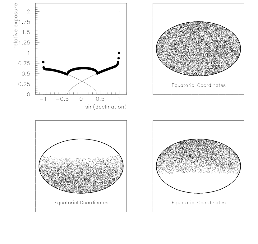
Figure 1: The upper left plot shows the declination dependence of the Auger Observatory’s relative exposure. The southern and northern sites are indicated separately by dots. The combined exposure function is marked with filled circles. The scatter plot in the upper right results from sampling an isotropic distribution and applying this Auger acceptance. There are 20,000 directions plotted, 10,000 from the southern site (shown separately in the lower left plot) and 10,000 from the northern site (lower right).

The upper left plot of figure 1 shows the resulting declination dependence for a site at $a_{0}=-35^{\circ}$ and another site at $a_{0}=+39^{\circ}$, which are the latitudes for the two Auger observatories. The detectors are assumed to be fully efficient out to $\theta_{m}=60^{\circ}$, and no arrival directions are counted from larger zenith angles. The combined exposure is also shown. The maximum is at the north pole direction, which is always detectable at the northern site, although the effective detector area is reduced by $cos(51^{\circ})$ for flux arriving from the north pole direction.

The lower plots in figure 1 are scatter plots of the accepted cosmic rays for each site, where directions have been sampled from an isotropic distribution but accepted according to each detector’s exposure. (A sampled cosmic ray direction is accepted if a randomly sampled number between 0 and 1 is less than the relative exposure $\omega$ for that direction.) There are 10,000 accepted arrival directions in each of those two plots. Shown in the upper right plot is the superposition of all 20,000 events from the combined observatory. The combined distribution is not uniform, but has the modest declination dependence indicated in the upper left plot.

3 Dipole sensitivity

The objective here is to study the sensitivity of a full-sky observatory to a dipole deviation from isotropy. How well can the dipole be measured? How does that accuracy depend on the number of arrival directions in the data set? How does it depend on the amplitude of the dipole anisotropy?

For a dipole deviation from isotropy, the cosmic ray intensity varies over the sky as

$$I(\vec{u})=\frac{N}{4\pi}(1+\alpha\vec{D}\cdot\vec{u}).$$

Here $\vec{u}$ is a unit vector defining the celestial direction, $\frac{N}{4\pi}$ is the average intensity, $\vec{D}$ is the dipole direction unit vector, and $\alpha$ is its (non-negative) amplitude. In order for the cosmic ray intensity to be nowhere negative, $\alpha$ must lie in the range $0\leq\alpha\leq 1$. The amplitude $\alpha$ gives the customary measure of anisotropy amplitude: $\alpha=(I_{max}-I_{min})/(I_{max}+I_{min})$.

The dipole can be recovered from the celestial intensity function by

$$\alpha\vec{D}=\frac{3}{N}\ \int I(\vec{u})\ \vec{u}\ d\Omega.$$

In our case, the observed intensity function consists of $N$ discrete arrival directions, each associated with a relative exposure $\omega_{i}$. The components of the dipole vector are then estimated by

$$\alpha D_{a}=\frac{3}{\cal N}\ \sum_{i=1}^{N}\ \frac{1}{\omega_{i}}\ u^{(i)}_{a},$$

where $u^{(i)}_{a}$ denotes a component of the $i$th vector, and $\cal N$ is the simple sum of the $N$ weights $\frac{1}{\omega_{i}}$. (These dipole components are linear combinations of the three spherical harmonic coefficients with $\ell=1$.)

To test this method’s sensitivity to a dipole of amplitude $\alpha$ when there are N directions in the data set, one can produce an ensemble of artificial data sets of this type (with random dipole directions $\vec{D}$). For each data set, use the above formula to estimate the dipole vector, and record the difference of the estimated $\alpha$ from the input alpha and also the angle between the estimated direction and the input dipole direction. These error distributions describe the measurement accuracy. The RMS deviation from the true $\alpha$ is a single number to characterize the amplitude measurement accuracy, and the average space angle error summarizes the accuracy of determining the dipole direction.

This procedure can be repeated for different values of $N$ and different values of $\alpha$. For any pair ($N,\alpha$) the ensemble of simulation data sets yields the amplitude resolution and direction resolution as above.

To generate an individual simulation data set, one samples $N$ arrival directions on the celestial sphere. First, a direction is sampled from the assumed celestial distribution with dipole deviation from isotropy. Then the detector acceptance is applied by rejecting the sampled direction if a random number is greater than the relative exposure $\omega$ for that direction. This continues until the data set has $N$ arrival directions. The data set then reflects both the presumed celestial anisotropy and the detector’s non-uniform exposure.

These methods yield the results summarized in figure 2. The number of arrival directions was increased by factors of two: $N$ = 250, 500, 1000, 2000, 4000, 8000, 16000, 32000. For each $N$, amplitudes were studied at $\alpha$ = 0.1, 0.2,…, 1.0.

The upper left plot of figure 2 shows that the amplitude is determined to an accuracy of about 0.1 with 250 directions, improving to approximately 0.01 with 32,000 directions.

Figure 2: Four plots that indicate how the sensitivity to dipole anisotropy depends on the number of arrival directions $N$ in the data set and the anisotropy amplitude $\alpha$. In the upper plots, the abscissa is the number of directions $N$. The left plot shows the RMS error in estimating the amplitude: the right plot shows the mean error in the measured dipole direction. Each column of points represent different amplitudes from 0.1 to 1.0. The open circle is $\alpha=0.1$ and the + mark is $\alpha=1.0.$ In the lower figures, the abscissa is amplitude $\alpha$ and the different points above each value represent different values of $N$ (increasing by factors of 2). The open circle is $N=250$, and the + is $N=32,000$. Multiplying the ordinate of a point in the lower right figure by $\sqrt{N}$ gives the number of sigmas deviation from isotropy. Each point is derived from an ensemble of 100 data sets.

The upper right plot shows the dipole direction resolution as a function of the number of arrival directions. The mean error is less than 10 degrees for all cases (250 directions or more) if the amplitude is nearly 1, and it is less than 10 degrees regardless of the amplitude if the number of directions is 16,000 or more.

The lower left plot shows that the mean dipole direction error decreases as the dipole amplitude increases. A strong amplitude yields a good direction determination even for a small number of directions in the data set. For example, with only 250 cosmic ray arrival directions, the dipole direction is determined to better than 20 degrees if the amplitude exceeds 0.5. To get that same resolution with $\alpha$=0.1, you need a data set with more than 4000 directions.

For a fixed number of arrival directions, the RMS error in the amplitude has little dependence on the amplitude. That is to say, you can distinguish amplitudes 0.85 and 0.90 as well as you can distinguish 0.10 and 0.15. For the purpose of detecting an anisotropy (as opposed to measuring it), the relevant quantity is the amplitude divided by the RMS error, which is the number of sigmas deviation from isotropy. That quantity increases with the amplitude $\alpha$. It can also be expected to increase in proportion to $\sqrt{N}$ as the number of arrival directions increases. The lower right plot shows that

$$\frac{\alpha}{\Delta\alpha}\approx 0.65\ \alpha\sqrt{N}.$$

For $N$=250, for example, the deviation from isotropy increases from 1-sigma to 10-sigma as $\alpha$ increases from 0.1 to 1.0. For $N$=8000, the range is from 6-sigma to 60-sigma. Etc.

To achieve a 5-sigma detection of a Compton-Getting anisotropy amplitude of 0.005 would require 2.4 million arrival directions. An anisotropy amplitude of 0.2 from a galactic halo distribution of sources, however, could be detected at the 5-sigma level with 1500 arrival directions.

4 Quadrupole sensitivity

A quadruople deviation from isotropy is characterized by an intensity function on the celestial sphere given by

$$I(\vec{u})={\bf Q}(\vec{u},\vec{u}),$$

where $\vec{u}$ is an arbitrary direction unit vector and ${\bf Q}$ is a symmetric 2nd order tensor. Its trace gives the monopole moment. Its other 5 independent components in any coordinate basis are determined from the $\ell=2$ spherical harmonic coefficients $a_{2m}$.

Denoting by $\xi_{i}$ the three eigenvalues of ${\bf Q}$ and the three (unit) eigenvectors by $\vec{q_{i}}$, the intensity function has the form

$$I(\vec{u})=\xi_{1}(\vec{q_{1}}\cdot\vec{u})^{2}+\xi_{2}(\vec{q_{2}}\cdot\vec{u})^{2}+\xi_{3}(\vec{q_{3}}\cdot\vec{u})^{2}.$$

To keep the number of studied variables manageable, consideration will be limited to axisymmetric oblate intensity functions, as might be expected from sources in the galactic disk or near the supergalactic plane. Let $\vec{q}$ denote the eigenvector that defines the symmetry axis, and let $\xi$ be the ratio of its eigenvalue to those in the symmetry plane, so the intensity function on the sphere is of the form

$$I(\vec{u})\propto\xi\ (\vec{q}\cdot\vec{u})^{2}+(\vec{u}_{\bot}\cdot\vec{u}_{\bot}),$$

where $\vec{u}_{\bot}\equiv\vec{u}-(\vec{u}\cdot\vec{q})\vec{q}$ is the part of $\vec{u}$ perpendicular to the symmetry axis, and $0\leq\xi\leq 1$. The anisotropy amplitude $\alpha$ is related to $\xi$ by

$$\alpha\equiv\frac{I_{max}-I_{min}}{I_{max}+I_{min}}=\frac{1-\xi}{1+\xi}\ \ \ \ \Leftrightarrow\ \ \ \ \xi=\frac{1-\alpha}{1+\alpha}.$$

The objective here is to test how accurately the anisotropy amplitude $\alpha$ and the symmetry axis direction $\vec{q}$ can be determined from a data set of arrival directions. How does the accuracy depend on the number of directions $N$ and on the amplitude $\alpha$?

The method of investigation is the same as for the dipole sensitivity study. For each pair ($N$,$\alpha$), an ensemble of simulation data sets are produced, each with a randomly chosen direction for its symmetry axis. For each data set, the arrival directions are sampled from the relative intensity function (with quadrupole anisotropy), and each direction is accepted with probability equal to the relative exposure $\omega$ evaluated at that direction.

The anisotropy amplitude $\alpha$ and symmetry axis direction $\vec{q}$ are estimated for each simulation data set. The tensor with components

$$S_{ab}\equiv\int\ I\ u_{a}u_{b}\ d\Omega$$

($u_{a}$ denoting a component of $\vec{u}$) has the same eigenvectors as $Q_{ab}$ and the components $S_{ab}$ can be estimated by

$$S_{ab}=\frac{1}{\cal N}\ \sum_{i=1}^{N}\ \frac{1}{\omega_{i}}\ u^{(i)}_{a}u^{(i)}_{b}.$$

The eigenvectors and eigenvalues of this symmetric matrix are then found. The symmetry axis is taken to be defined by the eigenvector with the smallest eigenvalue. Let $\Delta$ be that smallest eigenvalue subtracted from the average of the other two (which should be equal, corresponding to directions in the symmetry plane). The eigenvalue $\xi$ of the intensity tensor ${\bf Q}$ is given in terms of $\Delta$ by

$$\xi=\frac{2-10\Delta}{2+5\Delta}.$$

Then the anisotropy amplitude $\alpha$ is gotten by $\alpha=\frac{1-\xi}{1+\xi}$.

Results for ensembles with different ($N,\alpha$) values are presented in figure 3 in complete analogy with the dipole results presented in figure 2. The RMS error in the amplitude and the average space-angle error in the direction of the symmetry axis both decrease as $N$ increases. The symmetry axis is also seen to be better determined as the anisotropy amplitude increases for any fixed number of arrival directions $N$. The sensitivity for detecting anisotropy, as shown in the lower right plot, is given by

$$\frac{\alpha}{\Delta\alpha}\approx 0.45\ \alpha\sqrt{N}.$$

With the definition of anisotropy amplitude $\alpha\equiv\frac{I_{max}-I{min}}{I_{max}+I_{min}}$, detecting a quadrupole anisotropy requires more data than for a dipole anisotropy of the same amplitude. Twice as many cosmic ray arrival directions ($(.65/.45)^{2}\approx 2$) are needed for the same resolution.

Figure 3: Similar to figure 2 for dipole sensitivity, the plots in this figure indicate how sensitivity to quadrupole anisotropy depends on the size of the data set $N$ and the anisotropy amplitude $\alpha$. Symbol definitions are the same as in figure 2. Multiplying the ordinate of a point in the lower right plot by $\sqrt{N}$ gives the number of sigmas deviation from isotropy. Each point is derived from an ensemble of 100 data sets.

5 Spherical harmonics

For any data set of arrival directions (with full-sky exposure), the anisotropy patterns can be fully characterized by the set of spherical harmonic coefficients $a_{\ell m}$, in terms of which the intensity function over the sphere is given by

$$I(\theta,\phi)=\sum^{\infty}_{l=1}\ \sum^{\ell}_{m=-\ell}\ a_{\ell m}\ Y_{\ell m}(\theta,\phi).$$

The coefficients $a_{\ell m}$ are given by

$$a_{\ell m}=\int\ I(\theta,\phi)\ Y_{\ell m}(\theta,\phi)\ d\Omega.$$

Real-valued spherical harmonics are used in this paper, so the coefficients are real. The real-valued $Y_{\ell m}$ functions are obtained from the complex ones by substituting

$$e^{im\phi}\longrightarrow\left\{\begin{array}[]{ll}\ \sqrt{2}\ sin(m\phi)&m<0\\ \ 1&m=0\\ \ \sqrt{2}\ cos(m\phi)&m>0\end{array}\right.$$

For a set of $N$ discrete arrival directions with non-uniform relative expousre $\omega(\vec{u})$, the estimate for $a_{\ell m}$ is given by

$$a_{\ell m}=\frac{1}{\cal N}\sum_{i=1}^{N}\ \frac{1}{\omega_{i}}\ Y_{\ell m}(\vec{u}^{(i)})$$

where $\omega_{i}$ is the relative exposure at arrival direction $\vec{u}^{(i)}$ and $\cal N$ is the simple sum of the weights $\frac{1}{\omega_{i}}$.

The upper left plot in figure 4 shows a scatter plot of 2921 directions to extragalactic infrared sources with $z<0.01$, obtained from the NASA/IPAC Extragalactic Database (NED) [31]. There are certainly selection effects in these directions, but they are used here only as an example of an anisotropic celestial distribution. The spherical harmonic coefficients $a_{\ell m}$ for this distribution are plotted to the right of that scatter plot. There are 440 coefficients plotted for $1\leq\ell\leq 20$. Each set of $2\ell+1$ coefficients is plotted for each $\ell$ over an interval of 0.4 units on the abscissa. These $a_{\ell m}$ constitute a “fingerprint” of the anisotropy. They define a celestial intensity function that is a smoothed version of the scatter plot. The prominent coefficients $a_{11}$ and $a_{22}$ in this example result from the strong excess of the Virgo Cluster seen in the left central part of the scatter plot. Virgo is at declination 12.7 degrees and right ascension 187 degrees, and the $a_{\ell m}$ coefficients are derived here using that equatorial coordinate system (not the plotted supergalactic coordinate system).

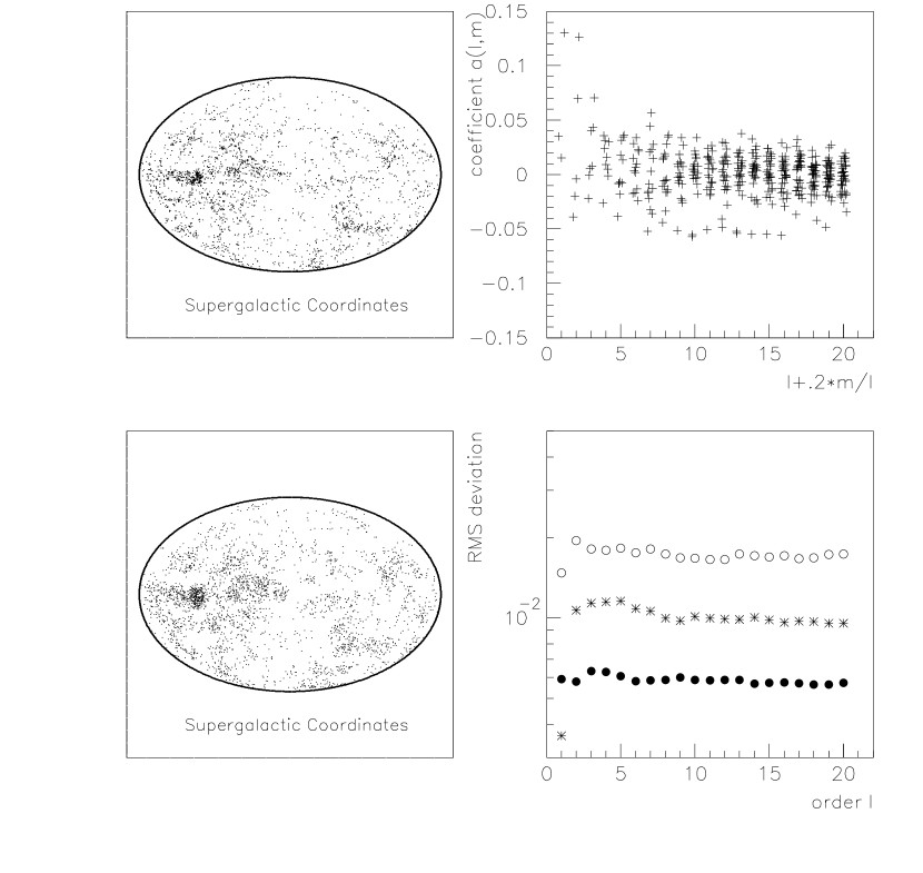
Figure 4: This figure indicates how anisotropy in arrival directions is characterized by spherical harmonic coefficients $a_{\ell m}$. The upper left plot is 2921 directions to extragalactic infrared sources. The upper right plot shows the spherical harmonic coefficients out to $\ell=20$ (using the equatorial coordinate basis). The lower left scatter plot shows arrival directions sampled from the smoothed celestial intensity function defined by those $a_{\ell m}$ coefficients (with the Auger exposure also imposed). Plotted at the lower right are the RMS differences between $a_{\ell m}$ coefficients derived from such sample simulations and those shown at the upper right. Open circles in the lower right correspond to a simulation with 250 sampled directions, asterisks to 1000 sampled directions, and the filled circles correspond to the simulation shown in the lower left with 2921 sampled arrival directions.

To illustrate how well the $a_{\ell m}$ coefficients characterize the anisotropy, arrival directions can be sampled from the intensity function that they define. The lower left plot is a scatter plot with the same number of directions (2921) based on the relative intensity function

$$I=\sum^{20}_{l=1}\sum^{\ell}_{m=-\ell}\ a_{\ell m}\ Y_{\ell m}.$$

The Auger exposure function has also been imposed. The lower left plot should not be identical to the upper left plot because of the Auger exposure simulation as well as the random sampling from the smoothed celestial anisotropy function. It clearly does have the same primary features, however.

The lower right plot in figure 4 summarizes how well the anisotropy is determined this way as a function of the number of arrival directions. The filled circles in that plot correspond to the displayed scatter plot with 2921 arrival directions. The $a_{\ell m}$ coefficients were derived from that simulation data set (using the relative exposure weights) and compared with those derived from the infrared source distribution. For each $\ell$, the RMS difference in the $a_{\ell m}$ values is plotted. One can see that the typical error in $a_{\ell m}$ is small compared to the significant coefficients in the upper right plot that characterize the anisotropy. The asterisks in the lower right plot are derived in the same way using a simulation with 1000 arrival directions. The open circles are the RMS coefficient differences resulting from a simulation with just 250 sampled arrival directions. The anisotropy fingerprint in this example is still measurable with 250 directions, although the RMS uncertainty in the $a_{\ell m}$ coefficients grows as $1/\sqrt{N}$ as $N$ decreases.

6 The angular power spectrum

The angular power spectrum is the average $a_{\ell m}^{2}$ as a function of $\ell$:

$$C(\ell)=\frac{1}{2l+1}\ \sum_{m=-\ell}^{\ell}\ a_{\ell m}^{2}.$$

The power in mode $\ell$ is sensitive to variations over angular scales near $1/\ell$ radians. The angular power spectrum provides a quick and sensitive method to test for anisotropy and to determine its magnitude and characteristic angular scale(s).

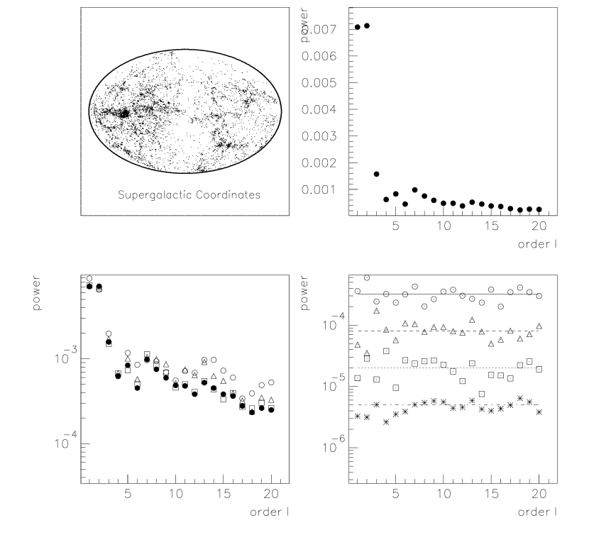
Figure 5: The upper left plot shows the celestial distribution of 7321 galaxy directions with $z<.01$ in supergalactic coordinates. The upper right plot is the power spectrum obtained using uniform exposure. The lower left plot compares this same power spectrum (filled circles) with power spectra obtained from simulation data sets of non-uniform exposure and reduced numbers of directions. Open circles result from a data set of 250 directions sampled from the galaxy distribution with the Auger relative exposure. The triangles pertain to a data set with 1000 directions, and squares to 4000 directions. The lower right plot shows the expected power resulting from the same type of finite sampling from an isotropic intensity. The symbols are the same as in the lower left plot, with asterisks representing a data set of 16,000 sampled directions.

As an example, consider the distribution of galaxies shown in the upper left plot of figure 5. These are all galaxies with redshift $z<0.01$ (also obtained from NED), and they are plotted in the supergalactic coordinate system. The Virgo cluster is the highest density region toward the left in this plot. There are 7321 galaxy positions plotted. The angular power spectrum (with no exposure correction) is shown out to $\ell=20$ in the upper right plot of that figure. There is excess power at all $\ell$-values, but especially for the dipole and quadrupole moments ($\ell$ = 1, 2) due to the high intensity from Virgo and other parts of the supergalactic plane.

The lower left plot in figure 5 indicates how sensitivity to the power spectrum is affected by the number of arrival directions (with non-uniform exposure as is expected for the Auger Observatory). Open circles in that plot are the power spectrum derived using a data set of 250 arrival directions. Those directions were obtained by randomly sampling from the 7321 galaxy directions (without replacement) and rejecting a sampled direction if a random number between 0 and 1 fell above the relative exposure $\omega$ evaluated at that direction. The 250 directions therefore represent a simulation Auger data set if each galaxy direction were to have equal probability of being a cosmic ray arrival direction. The open circles in the lower left plot are a decent approximation to the power spectrum (filled circles) of the “true” power spectrum defined by all 7321 directions with uniform exposure. The triangles in that plot represent the power spectrum for 1000 arrival directions sampled in the same way from the 7321, and the squares are obtained from 4000 sampled with the Auger exposure. It is clear that the approximation to the true power spectrum improves as the data set gets richer, but the gross information is already present with 250 arrival directions.

The lower right plot of figure 5 indicates how much power is expected due to fluctuations when directions are sampled from an isotropic intensity (and biased for the non-uniform expousre). The power is the same for all $\ell$-values and decreases like $1/N$ as the number of arrival directions increases. The power spectrum of the galaxy distribution is well above this noise level for all $\ell$-values for the cases $N$ = 4000 or 16,000. For 250 directions, only the first prominent harmonics in the lower left plot are clearly above the noise level indicated in the lower right plot.

Any class of candidate objects (e.g. active galaxies, or active galaxies with giant radio hot spots) has a celestial distribution that can be compared with a cosmic ray map when the whole sky has been surveyed with adequate sensitivity. Full information about the celestial distribution is provided by the set of coefficients $a_{\ell m}$. They can be tabulated out to $\ell=20$ in a list of 441 numbers (including the monopole). The angular power spectrum is a coordinate-independent gross summary of the features present in the celestial distribution. For example, you may learn from it that there is a large quadrupole moment, but you do not learn if the quadrupole has axial symmetry or the orientations of its principal axes. Full anisotropy information is given by the 441 $a_{\ell m}$ coefficients, not the 20 $C(l)$ powers.

The magnitude of the angular power $C(l)$ for larger $\ell$-values may contain useful information in the case that cosmic rays come from a limited number of discrete sources. The solid angle extent of the typical source affects the power at large values of $\ell$. Figure 6 displays an example in which there are 50 sources of equal flux with positions sampled randomly on the sky. Three different sky plots are shown, corresponding to different hypotheses about how much the arrival directions are dispersed from the source direction. In the upper left plot, sampled arrival directions are accepted only if they lie within $10^{\circ}$ of one of the sources. In the upper right plot, they are accepted only within 5 degrees of a source, and only within 1.5 degrees in the lower left plot. The graph in the lower right shows the power spectra for the three different simulations. The power at low $\ell$-values is governed by the chance pattern in the distribution of source positions. For $\ell\lower 2.15277pt\hbox{$\;\buildrel>\over{\sim}\;$}10$, however, the power clearly increases as the amount of source smearing decreases. The high end of the measurable angular power spectrum is sensitive to anisotropy structure on that finer scale.

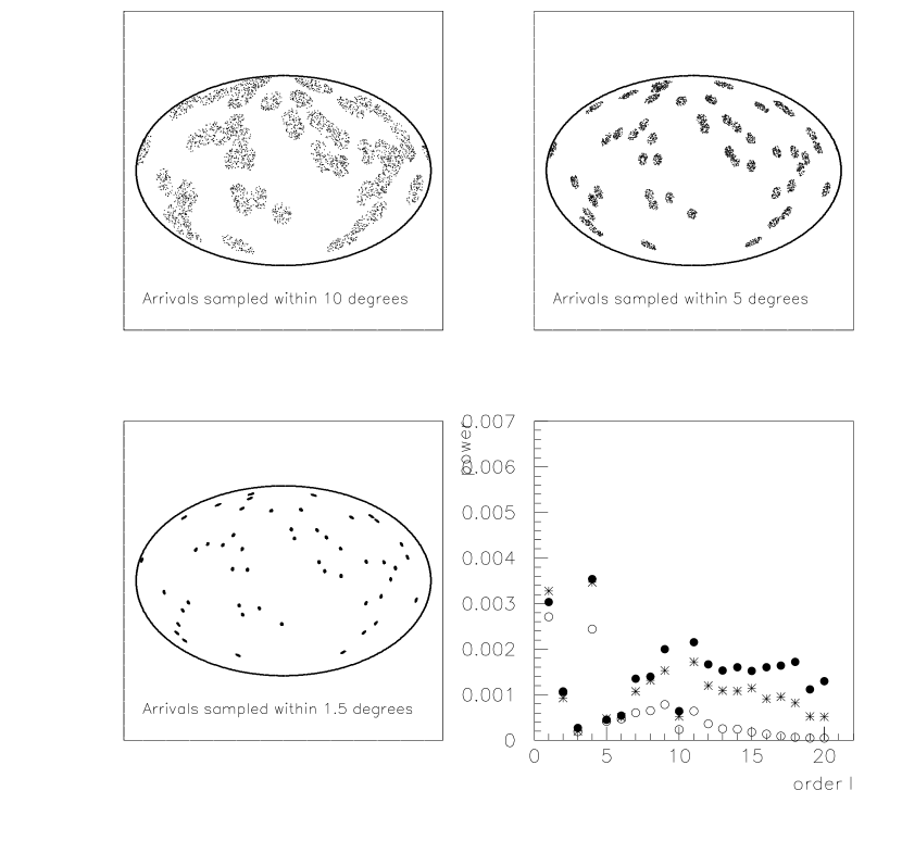
Figure 6: This study explores how the angular power spectrum from a set of discrete sources should change with the amount of smearing by magnetic dispersion. Fifty hypothetical source positions were sampled isotropically. A set of 4000 arrival directions were then sampled. An arrival direction was accepted if it were within an angular distance $\theta$ of any source (and was subjected to possible exclusion in accordance with Auger non-uniform exposure). Results for three different values of $\theta$ are shown: $\theta=10^{\circ}$ in the upper left, $\theta=5^{\circ}$ in the upper right, and $\theta=1.5^{\circ}$ in the lower left. Power spectra for the three cases are shown in the graph at the lower right (open circles for $\theta=10^{\circ}$, asterisks for $\theta=5^{\circ}$, and filled circles for $\theta=1.5^{\circ}$.

7 Discussion

There is great advantage in a cosmic ray observatory having exposure to the entire celestial sphere, especially if the relative exposure is nearly uniform. In that case, scatter plots of arrival directions are immediately interpretable, and eyeball evaluations can readily identify discrete sources or large-scale patterns. Discrete sources will be identified with equal sensitivity anywhere in the sky. If no such sources are found, the flux upper limits will be uniform over the sky.

At the highest energies there is no proven anisotropy. Unlike the COBE anisotropy analysis, it is not necessary to subtract a large known dipole pattern and a myriad of uninteresting foreground sources. Any cosmic ray deviations from isotropy will be of immediate interest. The search for cosmic ray anisotropy is more similar to the case of gamma-ray bursts, where expectations and early claims of anisotropy were not supported by additional data.

The role of an observatory is to map the sky and make the results available to the scientific community. This is highly challenging for an observatory without full-sky coverage. Measurements in that case are made with different sensitivity in different parts of the sky, and nothing at all can be said about a large hole where the exposure is zero. Certainly it is not possible to perform the full-sky integrations that are required to measure the multipoles of the celestial cosmic ray intensity. In this paper, frequent use is made of the inverse of the relative exposure, $1/\omega$. Such methods obviously fail if the relative exposure anywhere becomes infinitesimal or zero.

To underscore the difficulty of anisotropy analysis without full-sky coverage, one can cite the work by Wdowczyk and Wolfendale [32]. In that paper, the authors argue that the cosmic ray intensity measurements support a model of excess arrivals from equatorial galactic latitudes. The argument is based on the same data that two experimental groups had previously used in support of a gradient in galactic latitude that suggested an excess from southern latitudes relative to northern latitudes. In effect, because those northern detectors had poor exposure for southern galactic latitudes, Wdowczyk and Wolfendale were able to argue that the data supported a quadrupole distribution rather than a dipole distribution. Neither a dipole moment nor a quadrupole moment can be measured without full-sky coverage.

The techniques outlined in this paper pertain to any full-sky detector. Non-uniformity in celestial exposure is not hard to handle, provided it is well determined and there is adequate exposure to all parts of the sky. The true cosmic ray intensity is mapped with a sensitivity that depends primarily on the total number of detected arrival directions. This number $N$ is related to particle energy and observing time for any detector of known acceptance. This relationship for the Auger Observatory was given in the Introduction.

While complete information about anisotropy is encoded in the $a_{\ell m}$ coefficients (tied to some specified coordinate system), important gross properties of the anisotropy are characterized by the (coordinate independent) angular power spectrum $C(l)$. One can tell, for example, if there is a strong dipole or quadrupole moment. Such large-scale patterns are expected in many theories. It should be noted, however, that $C(1)$ gives the dipole moment but not its direction. It is obviously important whether the dipole points toward the galactic center, toward Virgo, toward Cen A, or in some unexpected direction. Similarly, all components of the quadrupole tensor are of interest, not just the average of their squares, $C(2)$. Nevertheless, the angular power spectrum provides a powerful tool for discriminating between viable and non-viable theories without detailed investigation. Also, the higher-order moments of the angular power spectrum can quantitatively characterize whatever clumpiness may exist in a map of arrival directions.

The techniques and examples mentioned in this paper are only representative of the powerful analysis methods that become possible with full-sky observatories. Data sets from such observatories will open a rich field of anisotropy study. The primary goal seen from the present time is the discovery of the highest energy cosmic ray origins. If that objective is accomplished (perhaps even before full-sky data sets are available), then the observed patterns from a known source distribution will be analyzed to infer properties of magnetic fields in the galactic halo and in intergalactic space.

A full-sky observatory has the ability to summarize completely the anisotropy information with the use of the spherical harmonic expansion coefficients $a_{\ell m}$. A table of coefficients (perhaps with multiple columns for different energy cuts) will provide the whole story. As has been done in this paper, those coefficients will be reliably corrected for the observatory’s non-uniform exposure. Detailed anisotropy analysis will no longer require privileged access to detector data. The published anisotropy fingerprint encoded in the $a_{\ell m}$ spherical harmonic coefficients can be matched against any theoretical suspect by any interested investigator.

Acknowledgement. It is a pleasure to thank Brian Fick for many helpful discussions about these matters.

References

- [1] J. Linsley and L. Scarsi, Phys. Rev. 128, 485 (1962).
- [2] J. Linsley, Phys. Rev. Lett. 10, 146 (1963).
- [3] D.J. Bird et al., Phys. Rev. Lett. 71, 3401 (1993).
- [4] K. Greisen, Phys. Rev. Lett. 16, 748 (1966).
- [5] G.T. Zatsepin and V.A. Kuzmin, Pis’ma Zh. Eksp. Teor. Fiz. 4 114 (1966) [JETP Lett. 4, 78 (1966).]
- [6] D.J. Bird et al., Ap. J. 441, 144 (1995).
- [7] N. hayashida et al., Phys. Rev. Lett. 73, 3491 (1994).
- [8] M. Takeda et al., Phys. Rev. Lett. 81, 1163 (1998).
- [9] C.C.H. Jui, highlight talk at the 26th Int. Cosmic Ray Conf., rapporteur volume (Salt Lake City), 1999.
- [10] M. Nagano and A.A. Watson, “Observations and Implications of the Ultra High Energy Cosmic Rays,” to appear in Rev. Mod. Phys. (July, 2000).
- [11] T. Abu-Zayyad, Proc. 26th Int. Cosmic Ray Conf. (Salt Lake City) 4, 349 (1999).
- [12] J.W. Cronin, Nucl. Phys. B. (Proc. Suppl) 28B, 213 (1992); The Pierre Auger Project Design Report (Fermilab, 1996).
- [13] M. Teshima et al., Nucl. Phys. B (Proc. Suppl.) 28B, 169 (1992); T. Aoki et al., Proc. 26th Int. Cosmic Ray Conf. (Salt Lake City), 4, 352 (1999).
- [14] R.E. Streitmatter, Proc. of Workshop on Observing Giant Cosmic Ray Air Showers from eV Particles from Space, eds: J.F. Krizmanic, J.F. Ormes, and R.E. STreitmatter AIP Conference Proceedings 433, 1997.
- [15] A.M. Hillas, Ann. Rev. Astron. Astrophys. 22, 425 (1984).
- [16] J.W. Elbert and P. Sommers, Ap. J. 441, 151 (1995).
- [17] P. Sommers, Particles and Fields, Proc. of the IXth Jorge Andre Swieca Summer School, eds: J.C.A. Barata, A.P.C. Malbouisson, S.F. Novaes, p.493 (World Scientific, 1998).
- [18] F.A. Aharonian, P. Bhattacharjee, and D.N. Schramm, Phys. Rev. D 46, 4188 (1992).
- [19] S. Yoshida, G. Sigl, and S. Lee, Phys. Rev. Lett. 81, 5505 (1998).
- [20] T. Weiler, Astropart. Phys., 11, 303 (1999).
- [21] G.R. Farrar, Phys. Rev. Lett. 76, 4111 (1996).
- [22] D.J. Chung, G.R. Farrar, and E.W. Kolb, Phys. Rev. D 55, 5749 (1998).
- [23] V. Berezinsky, “Ultra High Energy Cosmic Rays from Cosmological Relics,” eprint hep-ph/0001163 (2000).
- [24] A.M. Hillas, Nature 395, 15 (1998).
- [25] N. Hayashida et al., Phys. Rev. Lett. 11, 1000 (1996).
- [26] X. Chi et al., J. Phys. G 18, 539 (1992).
- [27] M.S. Briggs et al., Ap. J. 459, 40 (1996).
- [28] M. Tegmark et al., Ap. J. 468, 214 (1996).
- [29] G.F. Smoot et al., Ap. J. Lett., 396, L1 (1992).
- [30] M.S. Longair, High Energy Astrophysics vol. 2, p. 327 (Cambridge University Press, 1994).
- [31] NED=NASA/IPAC Extragalactic Database [http://nedwww.ipac.caltech.edu/].
- [32] J. Wdowczyk and A.W. Wolfendale, J. Phys. G 10, 1453 (1984).