Great Circle tidal streams:
evidence for a nearly spherical massive dark halo around the Milky Way

Abstract

An all high-latitude sky survey for cool carbon giant stars in the Galactic halo has revealed 75 such stars, of which the majority are new detections. Of these, more than half are clustered on a Great Circle on the sky which intersects the center of Sagittarius dwarf galaxy and is parallel to its proper motion vector, while many of the remainder are outlying Magellanic Cloud carbon stars. Previous numerical experiments of the disruption of the Sagittarius dwarf galaxy (the closest of the Galactic satellite galaxies) predicted that the effect of the strong tides, during its repeated close encounters with the Milky Way, would be to slowly disrupt that galaxy. Due to the small velocity dispersion of the disrupted particles, these disperse slowly along (approximately) the orbital path of the progenitor, eventually giving rise to a very long stream of tidal debris surrounding our Galaxy. The more recently disrupted fragments of this stream should contain a similar mix of stellar populations to that found in the progenitor, which includes giant carbon stars.

Given the measured position and velocity of the Sagittarius dwarf, we first integrate its orbit assuming a standard spherical model for the Galactic potential, and find both that the path of the orbit intersects the position of the stream, and that the radial velocity of the orbit, as viewed from the Solar position, agrees very well with the observed radial velocities of the carbon stars. We also present a pole-count analysis of the carbon star distribution, which clearly indicates that the Great Circle stream we have isolated is statistically significant, being a 5-6$\sigma$ over-density. These two arguments strongly support our conclusion that a large fraction of the Halo carbon stars originated in the Sagittarius dwarf galaxy.

The stream orbits the Galaxy between the present location of the Sagittarius dwarf, $16{\rm\,kpc}$ from the Galactic center, and the most distant stream carbon star, at $\sim 60{\rm\,kpc}$. It follows neither a polar nor a Galactic plane orbit, so that a large range in both Galactic $R$ and $z$ distances are probed. That the stream is observed as a Great Circle indicates that the Galaxy does not exert a significant torque upon the stream, so the Galactic potential must be nearly spherical in the regions probed by the stream. Furthermore, the radial mass distribution of the Halo must allow a particle at the position and with the velocity of the Sagittarius dwarf galaxy to reach the distance of the furthest stream carbon stars. Thus, the Sagittarius dwarf galaxy tidal stream gives a very powerful means to constrain the mass distribution it resides in, that is, the dark halo.

We present N-body experiments simulating this disruption process as a function of the distribution of mass in the Galactic halo. A likelihood analysis shows that, in the Galactocentric distance range $16{\rm\,kpc}<R<60{\rm\,kpc}$, the dark halo is most likely almost spherical. We rule out, at high confidence levels, the possibility that the Halo is significantly oblate, with isodensity contours of aspect $q_{m}<0.7$. This result is quite unexpected and contests currently popular galaxy formation models.

1 Introduction

One of the most intriguing puzzles of modern astronomy is the apparent existence of unseen mass on galactic and larger scales. Even for the Milky Way, our knowledge of the dark component is poor, the little known having been gleamed from indirect, mostly kinematic, probes.

The best constraints on the mass distribution in the Galaxy have been derived from the kinematics of tracers of the Galactic disk, in particular the H I gas, which samples the Galaxy from almost its center to the outermost parts of its disk. Indeed, the success of this technique in fitting the H I velocities at Galactic longitudes $\ell>30^{\circ}$ strongly suggests (Dehnen & Binney, 1998) that the Galaxy is axisymmetric at Galactocentric distances greater than $\sim 5{\rm\,kpc}$ — where most of the mass resides. Information on the vertical mass gradient has been obtained from the study of tracers of the Galactic spheroid (Wyse & Gilmore, 1986; Binney, May & Ostriker, 1987; Morrison Flynn & Freeman, 1990; Sommer-Larsen & Zhen, 1990; van der Marel, 1991; Amendt & Cuddleford, 1994; Morrison et al., 2000). Yet despite considerable observational and theoretical effort, the vertical structure of the spheroid component is still poorly constrained; dependent on the technique employed, the spheroid’s oblateness is found to lie in the range $0.5<q<1$. (It is usually assumed that the density of the spheroidal components of the Galaxy is of the form $\rho(s)$, where $s=(R^{2}+(z/q)^{2})^{1/2}$, and $R$, $z$ are Galactic cylindrical coordinates). This paucity of information on the vertical structure of the Galaxy, it transpires, is the primary cause of the large uncertainties on the Galactic mass models (Dehnen & Binney, 1998).

The above studies of the stellar spheroid do not, however, necessarily place strong constraints on the massive dark halo. This is because the stellar spheroid is a partially self-gravitating system, with its own density profile and kinematics. Also, at large radii, the stellar halo will not be dynamically relaxed, so we should expect to see a light distribution which reflects the formation process of this component (which may well have been quite different to that of the dark halo). Strong constraints on the dark material must therefore come from dynamical analyses. At large Galactocentric radii, satellites provide the only means to probe the dark halo (Zaritsky et al., 1989; Lin et al., 1999; Zaritsky & White, 1994). Within the end of a galaxy’s disk other analyses are possible, probing the self-gravity of stellar disks (Ueda et al., 1985), or of HI disks (Becquaert & Combes, 1997). For the case of our own Galaxy, it has already been possible to place constraints on the dark halo distribution through an analysis of the HI disk thickness (Olling & Merrifield, 2000), which suggests that the mass distribution is not substantially flattened, with $q\sim 0.8$.

In this contribution, we analyze kinematic and distance data of a group of newly-discovered stars that are part of a stream of material that has been tidally stripped from the Sagittarius dwarf galaxy. A stream gives much stronger constraints on the underlying mass distribution than does a uniformly distributed spheroid star population, as it implies a low velocity dispersion and a continuity between the stream members. It provides essentially the trace of an orbit through the Halo. The stream studied here is now distributed through the Halo between Galactocentric distances of $16{\rm\,kpc}$ to $\sim 60{\rm\,kpc}$, probing a region between the end of the Galactic disk, and the Magellanic clouds.

In section 2, we discuss the all-sky survey that reveals the Halo carbon star population; section 3 reviews previous analyses of the evolution of the Sagittarius dwarf galaxy and their predictions about its stellar stream; section 4 makes a simple first-pass comparison of the expected stream with the carbon star dataset and discusses the probability of a chance alignment. Section 5 presents a simple analytic argument to constrain the Halo shape and mass; section 6 provides a fuller analysis with the aid of N-body simulations covering a range of static Halo models. Finally, section 7 presents the conclusions of this work.

2 The Halo carbon star sample

The APM Halo carbon star survey reported in Totten & Irwin (1998), Totten, Irwin & Whitelock (2000) and Irwin & Totten (2000) is now almost complete. Palomar sky survey plates of the whole northern sky at Galactic latitudes $|b|\lower 2.15277pt\hbox{$\;\buildrel>\over{\sim}\;$}30^{\circ}$, as well as UK Schmidt Telescope plates covering most of the southern sky at latitudes $|b|\lower 2.15277pt\hbox{$\;\buildrel>\over{\sim}\;$}30^{\circ}$ (see Figure 1) have been scanned and analyzed to search for giant carbon stars (C-stars). These intermediate-age asymptotic giant branch stars are intrinsically luminous, rare ($\approx$1 per 200 sq. deg) and very red in optical passbands (Totten & Irwin, 1998), and can therefore easily be distinguished from other stellar species, making them a useful tracer of recent accretion events.

C-star candidates were selected according to their magnitudes and colors on APM scans of UKST and POSS1 sky survey photographic plates. Candidates were selected from color-magnitude diagrams by requiring that ${\rm B_{J}-R>2.5}$ and ${\rm 11<R<17}$, or the equivalent limits in the O and E POSSI passbands. The bright limit was chosen to minimize contamination by nearby disk, or thick disk carbon stars, since a typical carbon giant with absolute magnitude ${\rm M_{R}=-3.5}$, in general has to be in the approximate heliocentric distance range 10–100kpc to be included in the survey. The faint limit was chosen because a complementary deeper survey to an R-band magnitude of R=19, for a quasar program covering several thousand sq. deg of high latitude sky (Irwin et al. 1991) revealed no carbon stars fainter than R$\approx$16. Low or medium resolution spectra were obtained for all candidate C-stars, yielding spectral confirmation, and for nearly all confirmed C-stars, a further medium resolution spectrum was obtained to derive a radial velocity.

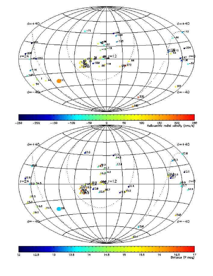
Figure 2: Aitoff projections of the positions of the $60$ Halo carbon stars in the sample with radial velocity measurements. The upper panel displays color-coded Heliocentric radial velocities, while the bottom panel shows the stellar distances, color-coded as a function of the observed apparent magnitude. The apparent magnitudes are true R-band magnitudes for those stars for which only R-band data is available, otherwise they are JHK-derived distances from Totten, Irwin & Whitelock (2000), converted to R-band magnitudes assuming ${\rm M_{R}=-3.5}$. Given a representative absolute magnitude of ${\rm M_{R}=-3.5}$ for these objects, the magnitude range displayed in the color wedge ranges from $12.5{\rm\,kpc}$ to $125{\rm\,kpc}$. The large point indicates the position and velocity of the central regions of the Sagittarius dwarf galaxy. Its heliocentric distance ($25{\rm\,kpc}$) is labelled on the diagram (all other points are labeled by the R-band magnitude of the corresponding C-star).

An Aitoff equal-area projection of the positions and velocities of all the high latitude carbon star giants with measured radial velocities is displayed in Figure 2; C-stars located within known Galactic satellite galaxies (LMC, SMC, Fornax, Carina, Sculptor) have been removed. The accuracy of the velocity data was estimated from fitting the peak of the cross-correlation function, and was better than $10{\rm\,km\,s^{-1}}$ for all stars.

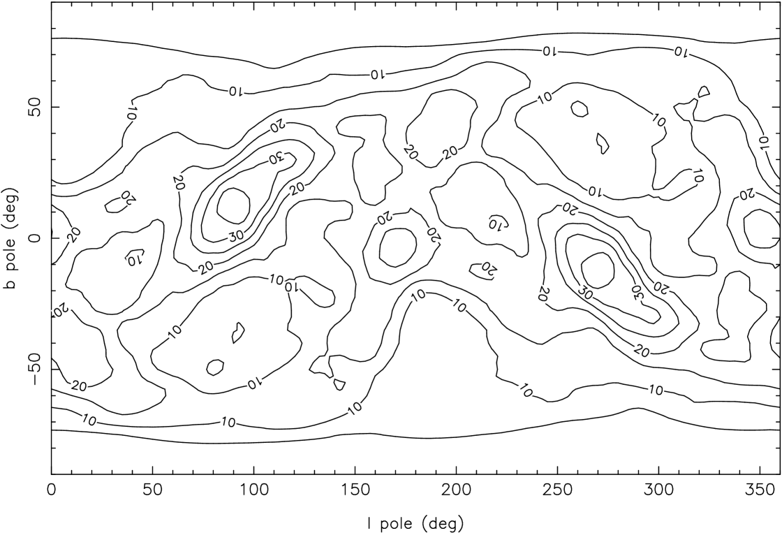
Figure 5: The contours represent the number of carbon stars from the APM survey, found within 10 degrees of putative Great Circle orbital paths. Each Great Circle track is defined by the Galactic coordinates of its pole. A 2.5 degree grid of these possible orbital poles was used as a basis for the contour map. The obvious concentration of carbon stars at $l=90^{\circ}$ , $b=13^{\circ}$ is coincident with the expected orbital pole of the Sagittarius dwarf galaxy, while that at $l=170^{\circ}$, $b=-3^{\circ}$ is a possible detection of stellar debris from the Magellanic Clouds. The observed $l,b$ of the carbon stars have been corrected to a Galactocentric coordinate system using approximate distances derived from their apparent R-band magnitudes.

Proper motion measurements for the majority of the Halo C-star sample showed that none of the APM-selected carbon stars had a significant proper motion (Totten, Irwin & Whitelock, 2000) ruling out the possibility of sample contamination by dwarf carbon stars. JHK photometric data have also been obtained for the majority of the Halo C-star in an attempt to derive approximate distances so as to correlate the optical R-band distance estimates with near IR estimates and at the same time obtain a clearer idea of the errors in estimating distance to isolated C-stars (Totten, Irwin & Whitelock, 2000). With the caveat that some C-stars are enveloped in dusty shells causing their distances to be overestimated, JHK photometry alone results in distance estimates with 2-$\sigma$ errors at the 25% level. Figure 5 of Totten, Irwin & Whitelock (2000) shows a good correlation between R-band and JHK distance estimates suggesting that for those C-stars without extant JHK photometry, R-band measures can suffice.

Visual inspection of Figure 2 clearly shows that the resulting C-star distribution is not at all random — either in position or in velocity — significant localized clumps are seen, with obvious correlations in both distance and radial velocity.

3 The Sagittarius dwarf galaxy and its tidal stream

The Sagittarius dwarf galaxy (Ibata, Gilmore & Irwin, 1994), is the closest satellite galaxy of the Milky Way; currently only $25\pm 1{\rm\,kpc}$ from the Sun, and $\sim 16{\rm\,kpc}$ from the Galactic center, it is near the point of its closest approach to the Galaxy. Such proximity to the Galactic center induces huge tidal stresses on the dwarf, which must lead to significant morphological modification if not its eventual destruction. The interaction is particularly interesting, as it provides a nearby, and hence easily observable, example of a system of merging galaxies.

Several numerical studies (Johnston, Spergel & Hernquist, 1995; Oh, Lin & Aarseth, 1995; Piatek Pryor, 1995; Velazquez & White, 1995; Johnston et al., 1999) have shown that dwarf satellite galaxies become elongated in the tidal field of their massive companion. Tidal debris from the satellite remains close to the plane of the orbit for several orbital periods if the host potential is sufficiently symmetric for the range of distances probed by the satellite orbit. Since the Sagittarius dwarf is on the Galactic minor axis, almost directly behind the Galactic center, as viewed from Earth, the projected elongation must be aligned with the proper motion vector (and the projection of the orbit) to very good approximation. The component of the proper motion of the central regions of the Sagittarius dwarf along the direction of the deduced orbit has been measured (Irwin et al., 1996; Ibata et al. , 1997), indicating that it is moving northwards with a transverse velocity of $250\pm 90{\rm\,km\,s^{-1}}$. A more recent analysis, using deep HST images close to the center of the dwarf, taken with an epoch difference of 2 years, gives a slightly higher velocity of $280\pm 20{\rm\,km\,s^{-1}}$ (Ibata et al., 2000a).

Ibata & Lewis (1998) performed numerical experiments to determine the likely structural evolution of the Sagittarius dwarf. Since ‘King models’ (King, 1962) fit the structure of present day dwarf spheroidal galaxies well (Irwin & Hatzidimitriou, 1995), they used these models to represent the structure of the initial pre-encounter dwarf galaxy. They set up a grid of 34 King models, sampling the plausible parameter space of concentration, central velocity dispersion and central density. The evolution of the models was calculated using an N-body tree-code algorithm (Richardson, 1993), which was modified to include the forces due to the assumed fixed Galaxy potential and due to dynamical friction, as approximated by the Chandrasekhar formula (Binney & Tremaine, 1987). The models, comprising either 4000 or 8000 particles, were evolved for 12 Gyr, a time equal to the age of the dominant stellar population in the Sagittarius dwarf (Fahlman et al., 1996). (The initial mean position and mean velocity of the models was obtained by integrating the orbit of a point-mass backwards in time for $12{\rm\,Gyr}$, with dynamical friction reversed).

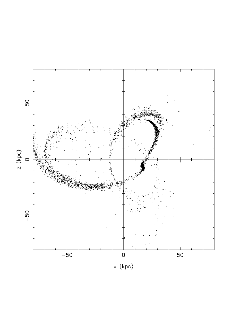
Figure 3: The remnant of one of the dwarf galaxy models from Ibata & Lewis (1998) (initial central density $\rho_{0}=2.0{\rm\,M_{\odot}}/{\rm\,pc}^{3}$, initial concentration $c=0.7$, initial central velocity dispersion $\sigma=40{\rm\,km\,s^{-1}}$) is shown in the $x$-$z$ plane of the Milky Way. The Galactic center lies at the origin, and the position of the Sun is at $x=-8{\rm\,kpc}$. The dwarf galaxy, evolved for $12{\rm\,Gyr}$ in the Milky Way potential model of Johnston, Spergel & Hernquist (1995) (a spherical halo has been used), has become significantly disrupted by the Galactic tides; long streams of material lead and trail the dwarf galaxy, which now contains $<60\%$ of the initial mass.

Figure 3 displays the end-point structure of one of the Ibata & Lewis (1998) dwarf galaxy models whose final velocity structure matches well the observed velocity dispersion and radial velocity profile of red-giant stars within $\sim 30^{\circ}$ of the center of that galaxy. In all of their N-body simulations, the modeled dwarf was found to give rise to streams of debris like those visible in in Figure 3; these contain more than $15\%$ of the initial galaxy, equivalent to a mass in the range $10^{7}{\rm\,M_{\odot}}\lower 2.15277pt\hbox{$\;\buildrel<\over{\sim}\;$}M_{debris}\lower 2.15277pt\hbox{$\;\buildrel<\over{\sim}\;$}2\times 10^{8}{\rm\,M_{\odot}}$. So a substantial stellar mass, comparable to the total mass of the Fornax dwarf spheroidal galaxy, should be detectable as a long stream of stars on the sky. However, the stream material will be mostly very faint, and its surface density will be low, approximately $15{\rm{\rm\,M_{\odot}}/arcmin^{2}}$. A practical method to detect such material is to search for intrinsically bright stars, such as carbon stars, that may trace the debris, which would be visible on large-area photographic surveys. Unfortunately, C-stars are quite rare; the Fornax dSph has $\sim 100$ C-stars (Azzopardi et al., 1998), so the debris tail of the Sagittarius dwarf should contain, to within an order of magnitude, a similar number of these stars.

4 The origin of the C-star stream

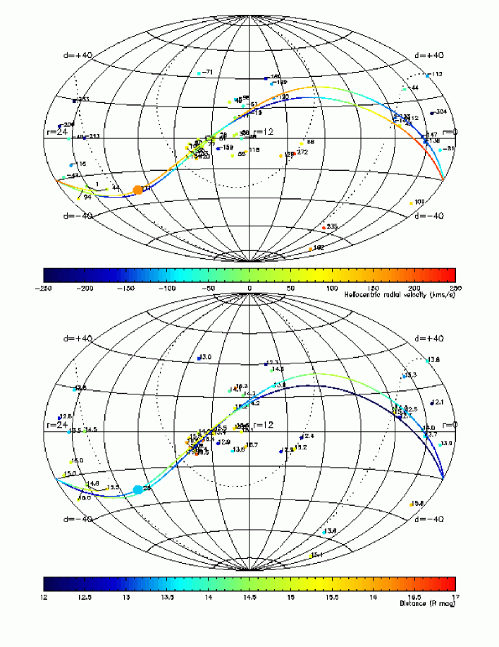
Figure 4: Projected orbit color-coded with velocities and distances overlaid on the data of Figure 2. The orbit has been integrated forwards and backwards in time for $1{\rm\,Gyr}$ (slightly more than two perigalactic passages) in the Galactic potential used by Johnston, Spergel & Hernquist (1995) and Ibata & Lewis (1998), which has a spherical halo component. The precession of the orbit in this model is due to the disk component, which was modelled as a Miyamoto disk. At large Galactocentric distance, this disk model provides unrealistically strong vertical potential gradients (the disk extends indefinitely). With a more realistic disk potential (as is used below) much less precession is seen in a Galactic potential with a spherical halo.

For simplicity, the simulations of Ibata & Lewis (1998) assumed a polar orbit. However, it was known even at that time that its orbit deviates substantially from polar. Lynden-Bell & Lynden-Bell (1995) estimated that the pole of its orbit is located at $(\ell=94^{\circ},b=11^{\circ})$, consistent with the HST proper motion measurement (Ibata et al., 2000a). Given the full three dimensional position and three dimensional velocity information on the center of the Sagittarius dwarf, we investigate its orbit in a standard Galactic potential. Figure 4 shows the projection of the orbit of the Sagittarius dwarf galaxy integrated in the spherical Galactic potential model of Johnston, Spergel & Hernquist (1995) (this was also the model used by Ibata & Lewis 1998). It is remarkable that the orbit of the Sagittarius dwarf in this “spherical cow” Galaxy model, where we have adjusted no free parameters, passes straight through the majority of the observed C-stars. The projected distance and radial velocity of the orbital path also give an acceptable fit to the C-stars. As the model potential used in Figure 4 is almost spherical at large radii, the orbital path is almost a Great Circle. Inspection of Figure 4 brings out clearly to the eye the stream-like distribution of the C-stars, which seem to follow a Great Circle on the sky.

To calculate the significance of this feature, we have performed a pole-count analysis (Johnston, Hernquist & Bolte, 1996) of the entire APM-selected high-latitude carbon star sample of 75 objects. The results are presented in Figure 5. Using the approximate R-band distance estimates for the carbon stars, the observed angular coordinates of the sample were corrected to a Galacto-centric coordinate system, assuming a solar distance of 8.5 kpc. There is a clear detection of a highly significant excess of carbon stars along a Great Circle with a pole at $90\pm 1$, $13\pm 1$ (plus the mirror pole at $270,-13$). This is within a few degrees of the expected orbital track of the Sagittarius dwarf from: its measured proper motion; its direction of elongation; and also from the analysis of Lynden-Bell & Lynden-Bell (1995) based on ”Halo” globular cluster systems. In addition, there is also another significant pole at $174,-3$ (plus mirror at $354,+3$) that is a possible detection of carbon stars associated with the orbit of the Magellanic Clouds (we defer discussion of that feature to a subsequent paper). It is also worth noting that the signature of both of these features is significantly enhanced when making use of the solar parallax correction described previously.

For a completely random distribution of carbon stars we would expect a fraction sin(10^∘) to lie within 10 deg of an arbitrary Great Circle. Yet 38 of the 75 faint high latitude carbon stars lie close to the Sagittarius dwarf track, and 28 out of the 75 lie close to the Magellanic Cloud (MC) track, compared with an expected number of $\approx$13. However, this would be a naive statistical assessment for several reasons. First, if a large fraction of the carbon stars do belong to Sagittarius (and the Magellanic Clouds) then the ’background’ level estimated above would clearly be an overestimate. Second, the high latitude sample is not yet complete particularly in the Southern part of the survey leading to uneven coverage and hence non-uniformity of the ’background’. Third, the lower Galactic latitudes are almost completely absent from the carbon star distribution, weighting against Great Circle orbital tracks close to the Galactic equator. Indeed this latter effect can be clearly seen in the general trend of the contours with respect to Galactic latitude. Therefore, taking a more empirical approach, the general ’background’ level of the contour distribution well away from the Sagittarius dwarf and MC poles, but within 60 degrees of $b=0$, averages around 10 counts, with a 1-sigma variation of approximately 5 counts (we will return to the issue of the background “noise” from other accretion events in §6). This suggests that the postulated tidal debris for the Sagittarius dwarf and MC tracks are significant at approximately 5-6 sigma and 3-4 sigma levels respectively, thereby clearly revealing for the first time direct evidence of giant arcs of stellar tidal debris associated with Sagittarius dwarf and possibly also for the MCs.

Thus it appears highly likely that a significant fraction of the Halo C-stars, formed and were once bound to the Sagittarius dwarf galaxy. The non-uniform sky coverage of our survey does not affect this result. We performed Monte Carlo simulations of a random Halo carbon star population (drawn from a spherical logarithmic model) windowed by the field distribution of plate material shown (for the Southern sky) in Figure 1. In 1000 random simulations there were no instances of a peak as significant as that seen in Figure 5. It is, however, unclear to us how to assess the significance of our putative Sgr stream detection against a possible arbitrarily non-uniform Halo distribution. Certain types of Halo sub-structure, such as the majority of the Halo being in randomized thin ”spaghetti-like” distributions, would have little effect on the significance of the detected peak since the effective smoothing scale around each trial Great Circle covers a broad band of some $\pm 10$ degrees. This is clearly not the case if the Halo carbon star population is composed of a small number of large scale streams, whose presence would make the pole-count distribution lumpier and so lower the significance of the observed pole-count peaks. So to avoid accepting the existence of the two large streams, one has to postulate the existence of a background of large scale streams. In this case, decomposing the Halo distribution into the minimum number of streams required to ”fit” the observables would seem to be the best way to proceed. However, we have no a-priori knowledge about the maximum number of streams we may accept (indeed, current cosmological simulations predict that hundreds of dwarf galaxy sized dark matter clumps inhabit the halos of giant galaxies like the Milky Way, Moore et. al 1999), so in this situation it is not possible to assess the significance of the observed pole-count peaks. It is worth stressing at this point that the Great Circle Pole count method only uses two of the phase space constraints (distance makes only weak a contribution). As we show in Figure 4, the distance and radial velocity information corroborate the angular information. A better method needs to be developed that uses all of the available information rather than some of it; this will be done below in §6 by comparison to N-body simulations.

5 Halo constraints: a “back of the envelope” approach

In the simulations below, the tidal stream of the Sagittarius dwarf is a very long-lived feature, remaining confined as a continuous narrow feature for much longer than the age of the Universe. The tidally stripped particles have a low velocity dispersion (like their progenitor), and once they drift beyond close proximity to the remaining bound clump, the only significant gravitational influence they feel is that of the Galaxy. These properties make the stream material remain close to the locus of the orbit of a point-mass representing the center of mass of the dwarf galaxy model. It is clear that this approximation holds best if the progenitor has low mass (as suggested by the work of Gómez-Flechoso, Fux & Martinet, 1999).

We may obtain a simple estimate of the apogalactic distance of the orbit of the Sagittarius dwarf, assuming a simple spherical logarithmic potential model for the Halo $\Phi(r)={v_{0}^{2}}\ln(r)$, where $v_{0}$ is the circular velocity of the Galaxy. Taking a perigalactic distance of $16{\rm\,kpc}$, and a present velocity of $330{\rm\,km\,s^{-1}}$, we find the roots of the equation:

$$u^{2}+{{2[\Phi(1/u)-E]}\over{L^{2}}}=0,$$

(Equation 3-13 from Binney & Tremaine 1987), where $u=r^{-1}$, $E$ is the energy per unit mass of the object, and $L$ is its angular momentum. This simple calculation yields an apocenter distance of $r_{apo}=56{\rm\,kpc}$ (taking $v_{0}=200{\rm\,km\,s^{-1}}$) and $r_{apo}=42{\rm\,kpc}$ (with $v_{0}=220{\rm\,km\,s^{-1}}$). We see from this that the Sagittarius dwarf galaxy is capable of reaching the distances where the C-stars are found (see §3), and also that the measured velocity of the dwarf galaxy provides a means to probe the mass of the Halo (parametrized in this example as a circular velocity).

The discussion in §4 showed that there is a strong over-density of C-stars on a Great Circle that happens to coincide with the projection of the expected orbit of the Sagittarius dwarf in a standard Galaxy potential with a spherical halo. In a spherical potential, the angular momentum of an orbiting test particle is conserved, so there is no precession; so all orbits follow Great Circles as viewed from the center of the potential. In an axisymmetric (or more complex) potential, particles on orbits that are neither polar or in the equatorial plane experience a torque which leads to a precession; viewed from the center of the potential one generally will not perceive a Great Circle path. Therefore, the fact that the C-star stream follows a Great Circle immediately tells us that the Galactic potential, in the regions occupied by the stream, cannot be far from spherical. To illustrate this point we consider orbits in the flattened logarithmic potential $\Phi(R,z)={v_{0}^{2}}\ln((R^{2}+z^{2}/q^{2})^{1/2})$. In this potential, an orbit which is close to being circular precesses at a rate of approximately (Steiman-Cameron & Durisen, 1990):

$$\omega_{p}(r)=-{{3}\over{2}}\Big{(}{{v_{0}}\over{r}}\Big{)}{{(1-q^{2})}\over{(1+2q^{2})}}\cos(i);$$

this approximation is accurate to $\sim 10$% at $q=0.8$. The orbit of the Sagittarius dwarf is not really circular, so the preceding expression will give only a rough approximation to the precession rate. We take an average distance of $r=30{\rm\,kpc}$ for this calculation, and $i=77.5^{\circ}$. The precession rate for even a slightly flattened model, with $q=0.8$, is very fast, $\approx 60^{\circ}/{\rm\,Gyr}$; so even in this mildly flattened halo, we should not expect to see a long coherent Great Circle stream if that stream has taken a few ${\rm\,Gyr}$ to disperse. Clearly, our data have the potential to strongly constrain the shape of the dark halo of the Milky Way. Note that, unlike the case of polar ring galaxies (Sackett & Sparke, 1990), the self-gravity of the stellar stream is negligible.

In the next section we undertake a more quantitative analysis, to find the Galaxy models allowed by the data.

6 Halo constraints: N-body simulations

The previous analysis clearly demonstrates that a substantial fraction of giant carbon stars recently identified in the Galactic halo are both spatially and kinematically consistent with them being members of the tidal stream torn from the Sagittarius Dwarf Galaxy. To employ these tracers in constraining the mass distribution within the Galactic halo, however, it is important to understand the demise of the Sagittarius Dwarf in a variety of models of the Galactic potential. To this end, a suite of numerical simulations were undertaken.

6.1 Galactic potential model

The Galactic mass models of Dehnen & Binney (1998), the most realistic models currently available, were used to represent the Milky Way in our simulations. These models contain 5 components: a thin disk, a thick disk, an inter-stellar medium, a bulge and a halo, with parameters that are fit to available observational data. We find that the path of the stream is almost entirely insensitive to the choice of (plausible) parameters of the first four of these components, which is not surprising since the Sagittarius dwarf orbits at large Galactocentric distance. For those four components, we choose the parameters of the Dehnen & Binney (1998) model 2, which gives a marginally better fit to the their compilation of available data than do their other standard models. The stream, however, is sensitive to the Halo parameters. The form of the Halo mass distribution taken by Dehnen & Binney (1998) is:

$$\rho(R,z)=\rho_{0}\Big{(}{{s}\over{r_{0}}}\Big{)}^{-\gamma}\Big{(}1+{{s}\over{r_{0}}}\Big{)}^{\gamma-\beta}e^{-s^{2}/r^{2}_{t}},$$

where $r_{0}$ is the core (or scale) radius, $r_{t}$ is the truncation radius, $\gamma$ is the power-law index in the core, and $\beta$ the power-law index outside the core. Based on the kinematics of the outer satellites of the Milky Way (Zaritsky et al., 1989), we assume that the Halo truncation radius is well outside the apogalactic distance of the orbit of the Sagittarius dwarf. The parameters $\beta$, $\gamma$, and $r_{0}$ have to be chosen simultaneously to give rise to a realistic rotation curve. We have chosen to work with two quite different families of Halo models. The first of these (H1) is motivated by observations of galaxies with extended HI distributions, these all show flat rotation curves, implying that $\beta=2$. For these Halo models we take a small ($r_{0}=3{\rm\,kpc}$) constant density ($\gamma=0$) core. The resulting Galaxy rotation curve is displayed in Figure 6. Our other family of Halo models (H2) is motivated by the cosmological simulations of Navarro, Frenk & White (1997). Their “universal profile” is equivalent to setting $\gamma=1$ and $\beta=3$. They also predict the size of the scale radius $r_{0}$ as a function of galaxy mass; assuming that the Milky Way has a mass interior to $200{\rm\,kpc}$ of $10^{12}{\rm\,M_{\odot}}$ (see Zaritsky 1999 and references therein), then $r_{0}\sim 20{\rm\,kpc}$ (for the case of the currently popular $\Lambda$CDM cosmology). The Galactic rotation curve of this model is also displayed in Figure 6.

The remaining two parameters, which are to be explored, are the the central density (which we rearrange into the more intuitive $v_{c}(50{\rm\,kpc})$, the circular velocity at $50{\rm\,kpc}$) and the flattening $q_{m}$.

A computer algorithm for calculating the potential and forces due to these mass models was kindly provided by Dr. W. Dehnen, and was integrated into our N-body workhorse, PKDGRAV, a highly efficient and scalable N-body code (Stadel & Quinn, 2000). In all the following simulations we maintained accurate forces by using an opening angle of $0.75$ and expanding the cell moments to hexadecapole order. Two body relaxation was suppressed by using a spline softening of 10 pc, such that the inter-particle forces are completely Newtonian at 20 pc. A variable time-step scheme is used based on the local acceleration, $\Delta t<\eta\sqrt{|\Phi|}/a$, and density, $\Delta t<\eta/\sqrt{G\rho}$, with the accuracy parameter $\eta=0.03$ (Quinn et al., 1997). Typically we used 100000 base steps to integrate 12 Gyr. With the variable time-steps, this was equivalent to taking $5\times 10^{7}$ time-steps.

For each Galactic model, the current center-of-mass of the Sagittarius dwarf was orbited backwards for 12 Gyr. At this ‘initial position’, the dwarf is modeled as a King profile. This self-gravitating system is then integrated forwards for 12 Gyr within the fixed Galactic potential. Our aim is to compare the structure and kinematics of the resulting stream at the present day to the observed C-star distribution. Clearly, the final structure of the dwarf galaxy remnant and its stream depends on the assumed initial distribution function, so we next discuss our choice of model.

6.2 The initial model of the Sagittarius dwarf

Our choice of a King model for the initial distribution function is supported by the fact that isolated Galactic dwarf spheroidal galaxies conform well to this model (Irwin & Hatzidimitriou, 1995). King models can be parametrized in terms of a total mass, a concentration, and a half-mass radius.

We first address the issue of the initial mass $M_{0}$ of the object. Previous numerical studies (Johnston, Spergel & Hernquist, 1995; Velazquez & White, 1995; Ibata & Lewis, 1998; Gómez-Flechoso, Fux & Martinet, 1999) were unable to find a low-mass model robust enough to survive the Galactic tides for $\sim 10{\rm\,Gyr}$, and display a final half-mass radius as large as the observed $r_{1/2}=550{\rm\,pc}$ (for instance, the best model of Gómez-Flechoso, Fux & Martinet 1999 has a half mass volume a factor of 100 smaller than the observed half brightness volume). Recently, a new model has been proposed by Helmi & White (2000). Their model 1 gives a good representation of available observations of the central of the dwarf galaxy. However, their model predicts that the tidal debris stars should outnumber remnant dwarf galaxy stars by a factor of 8. We make a provisional estimate of the total N-type carbon star population in the central regions of the Sagittarius dwarf of $N_{\rm C-star}\sim 100$, derived by scaling the Whitelock, Irwin & Catchpole (1996) survey to the total area $22^{\circ}\times 7^{\circ}$ (Ibata et al. , 1997; Cseresnjes, Alard & Guibert, 2000) over which the dwarf is now known to extend. The fraction of mass disrupted from the dwarf galaxy is then strongly constrained by the observed Halo C-star distribution presented in Figure 2; we use this argument in a companion paper (Ibata et al., 2000c) to show that the Helmi & White (2000) study is inconsistent with the observed carbon star distribution, as it predicts too much tidal debris.

Zhao (1998) suggested that an encounter with the LMC $2{\rm\,Gyr}$ ago could have deflected the Sagittarius dwarf from a longer period orbit into the current, tidally-disruptive, short-period orbit. However, the extended forward and backward arms of disrupted C-stars argues against that possibility as the observed structure is consistent with the slow loss of material over many close encounters with the Milky Way. Another alternative, suggested by Jiang & Binney (1999) is that the dwarf galaxy began by being very massive, up to $10^{11}{\rm\,M_{\odot}}$; orbital evolution through dynamical friction plus tidal dissolution could have led to its present, much reduced, state. This scenario now also appears highly unlikely in the light of the Halo C-star distribution presented in Figure 2: if the present day Sagittarius dwarf is a mere 1% remnant, we would expect to see some $\sim 3000$ C-stars and a substantial population of globular clusters (since the present day Sagittarius also contains 4 globular clusters) distributed in the Halo, quite unlike what is observed. It should be noted that this argument may be weakened if the original dwarf galaxy had a strong gradient in mass to light ratio, so that the luminous material was most centrally concentrated, and therefore the last part to be dissolved.

In summary, we feel that a more conservative model with a modest initial mass in the range $10^{8}{\rm\,M_{\odot}}$ to $10^{9}{\rm\,M_{\odot}}$ (Ibata et al. , 1997; Ibata & Lewis, 1998), requiring less dark matter in the dwarf galaxy, provides a better representation of our current knowledge of this system.

Our previous N-body work on this interaction Ibata & Lewis (1998) probed a large range of the parameter space of initial King models. We found that only low concentration models ($c<1$) can give rise to low concentration remnants (which is required by the observations). (Following Binney & Tremaine (1987), we define $c=\log_{1}0(r_{t}/r_{0})$, where $r_{t}$ is the tidal radius and $r_{0}$ is the King radius of the system). For our dwarf galaxy model D1 we have therefore chosen $c=0.5$ for the initial King profile. The remaining parameter that must be chosen is the half-mass radius. Our earlier work also showed that the minor-axis half-mass radius tends to decrease as disruption proceeds, thus requiring a large initial half-mass radius to be consistent with the observed $0.55{\rm\,kpc}$ minor-axis half-brightness radius. The choice of $r_{1/2}=0.5{\rm\,kpc}$, is a compromise between survivability and final size. More extended models tend to disrupt too quickly to leave a remnant at the present day. While these models with initial $r_{1/2}=0.5{\rm\,kpc}$ do survive in the Galactic potentials described above, they give rise to final half-mass radii that are a factor of $\sim 2$ smaller than the observed $0.55{\rm\,kpc}$ minor-axis half-brightness radius (physically, the disruption rate is, of course, proportional to the density – so the discrepancy is worse). The total mass of model D1 is $10^{8}{\rm\,M_{\odot}}$. Our second dwarf galaxy model D2, is a copy of the Helmi & White (2000) model I, which give a final structure similar to what is observed, but at the expense of a disruption rate apparently inconsistent with the observations. This model has initial half-mass radius $r_{1/2}=1.0{\rm\,kpc}$, and concentration $c=0.7$, giving a total mass of $5.74\times 10^{8}{\rm\,M_{\odot}}$.

Thus neither of the models we use for the initial state of the Sagittarius dwarf progenitor is entirely satisfactory. However, by examining the differences between the simulation results with model D1 (which is too compact) and model D2 (which is too susceptible to disruption) we shall be better able to understand the actual evolution of the dwarf galaxy.

6.3 Simulation results

The dwarf galaxy model is integrated forward through the Galactic potential for $12{\rm\,Gyr}$. The mass of these dwarf galaxy models is such that dynamical friction does not significantly influence the evolution of the orbit, so this effect is neglected. In the majority of models, the dwarf galaxy was represented by $10^{4}$ particles, although to ensure that the results were not biased by the number of particles employed, several simulations were repeated with $10^{5}$ particles. To compare the simulations to the observed C-stars (which are stars of intermediate age, $T\lower 2.15277pt\hbox{$\;\buildrel<\over{\sim}\;$}6{\rm\,Gyr}$) we have selected for comparison only those simulation particles that were located within a sphere of radius $5{\rm\,kpc}$ from the remnant center at the simulation time $6{\rm\,Gyr}$ before the present. Any population that was disrupted at earlier epochs would be too old to be detectable via C-star tracers.

To summarize, we employed two different families of Halo models, H1 and H2. Each of these Halo models was investigated with three values of the circular velocity ($v_{c}(50{\rm\,kpc})=200{\rm\,km\,s^{-1}},220{\rm\,km\,s^{-1}},240{\rm\,km\,s^{-1}}$) and with eleven values of the Halo density flattening ($q_{m}=0.5,0.55,\dots,1.0$). Both dwarf galaxy models D1 and D2 were evolved in these 66 Galactic potentials, for a total of 132 simulations.

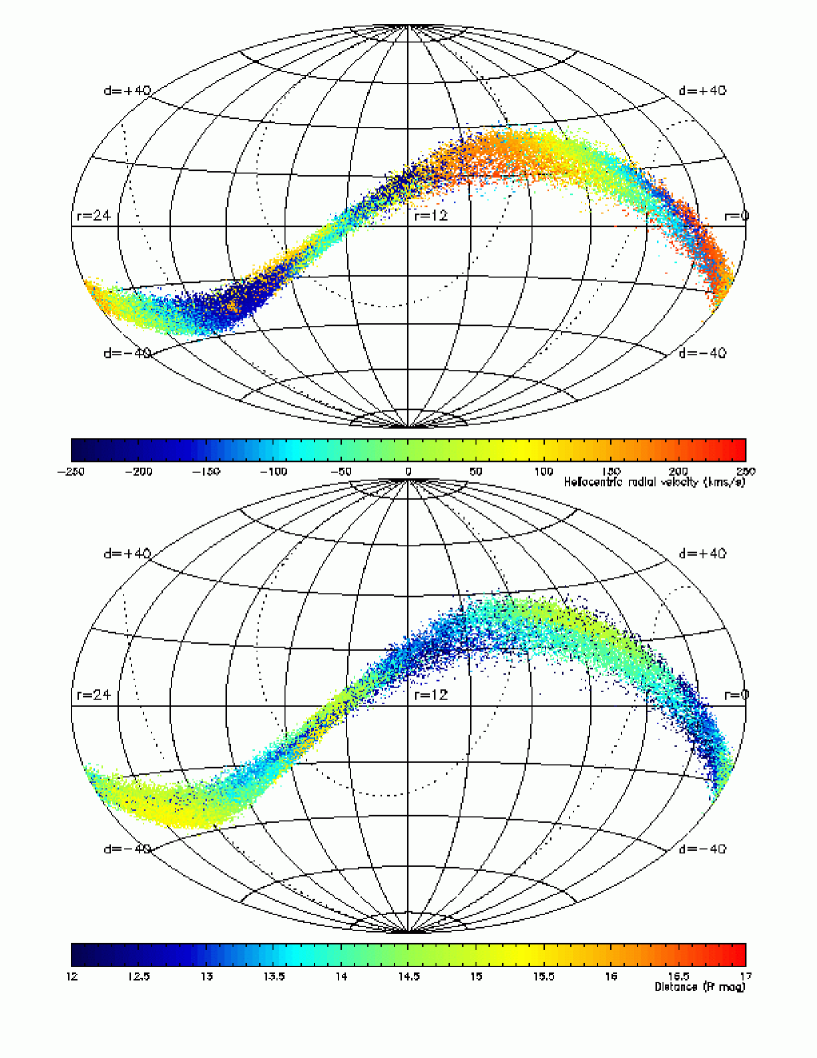
Figure 7: The end-state of the simulation (at $T=12{\rm\,Gyr}$) of the dwarf galaxy model D1 (originally containing $10^{5}$ particles) in the Galactic potential model H1 with $v_{c}=220{\rm\,km\,s^{-1}}$, and $q_{m}=1.0$ is shown. The distribution of debris on the sky follows quite closely a Great Circle.

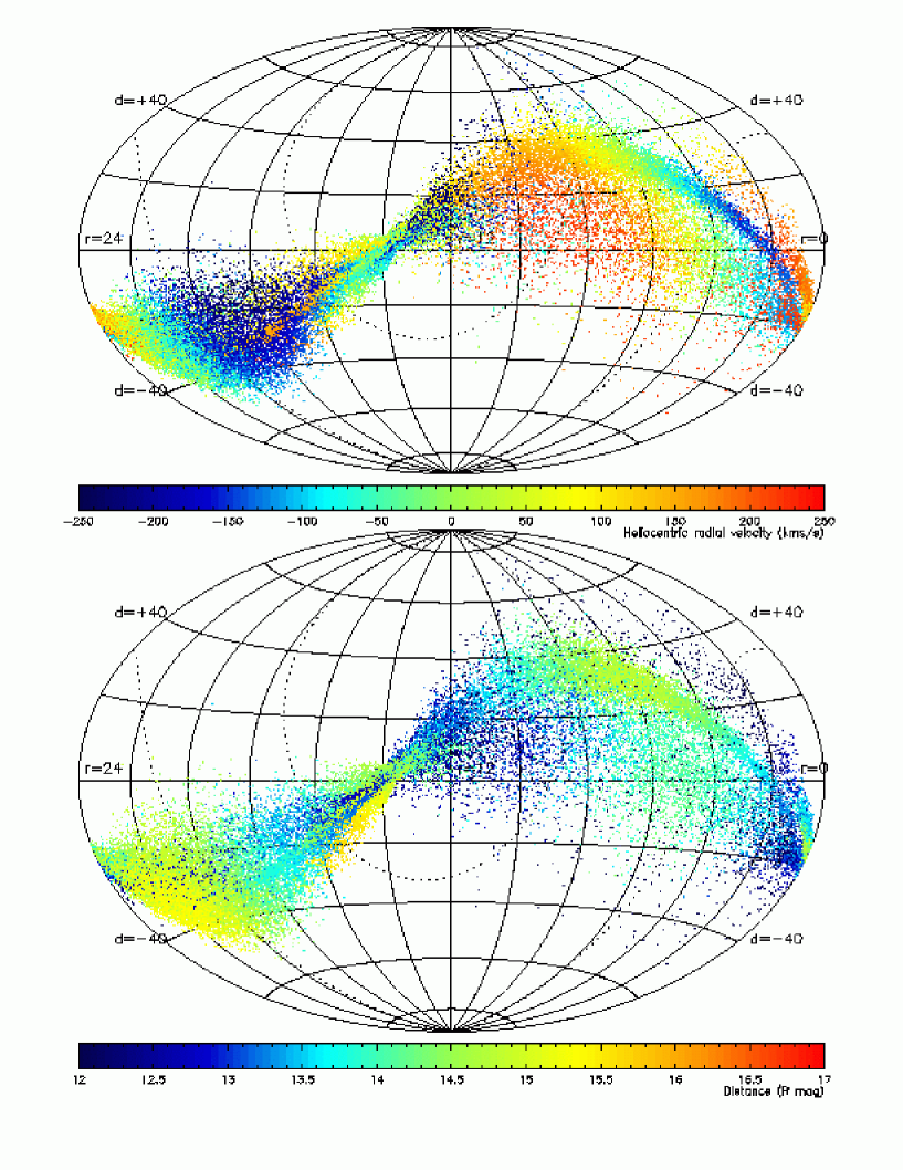
Figure 8: Same as Figure 7, but with $q_{m}=0.9$. A significant amount of material is now precessed away from the Great Circle stream.

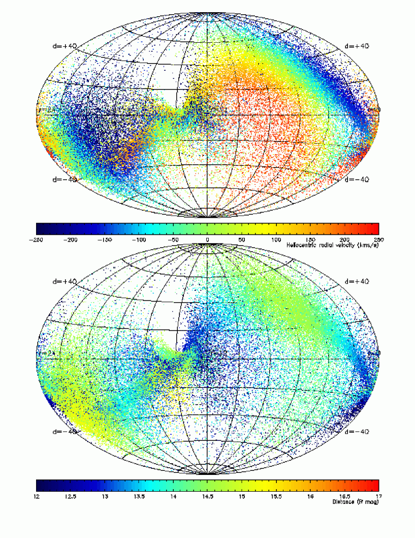
Figure 9: Same as Figure 7, but with $q_{m}=0.75$.

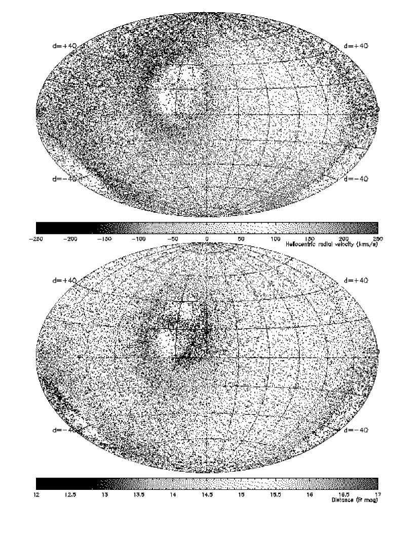
Figure 10: Same as Figure 7, but with $q_{m}=0.5$. The tidally disrupted debris from the dwarf galaxy has suffered so much precession in this flattened potential that no sign of a Great Circle stream remains. Apart from the two obvious holes around the Galactic poles, the distribution of stars on the sky is close to isotropic. The large velocity dipole, which is more obvious in this plot than in the preceding three, is simply due to the Solar reflex motion.

Figures 7 to 10 show the end-state of the dwarf galaxy evolved in Milky Way potential models H1 with $v_{c}(50{\rm\,kpc})=220{\rm\,km\,s^{-1}}$; the Halo models are progressively flatter from Figure 7 ($q_{m}=1$), Figure 8 ($q_{m}=0.9$), Figure 9 ($q_{m}=0.75$), to Figure 10 ($q_{m}=0.5$). Expectations regarding the effect of the Halo flattening on the observed structure of the stream (§5) are clearly confirmed. A visual comparison of these diagrams with the data (Figure 2) also appears to bear out our earlier deduction that the Halo cannot be substantially flattened: Figures 7 and 8 seem to be much better approximations to the data than Figures 9 and 10.

6.4 Quantitative comparison to data

A straightforward way to compare our simulation results to the observed C-star distribution is to compute the likelihood of the various models given these data. We apply Gaussian smoothing to each simulation particle, using the observational uncertainties in velocity ($\Delta v=10{\rm\,km\,s^{-1}}$) and distance (${\rm\Delta R=0.3mag}$), and we further smooth in right ascension and declination with a dispersion equal to approximately half the width of the simulated stream ($\Delta\alpha=5^{\circ}$, $\Delta\delta=5^{\circ}$); this gives a better approximation to the underlying probability distribution function $l_{m}(\alpha,\delta,{\rm R},v)$ of model $m$. The likelihood of model $m$ is then the product of the likelihoods of the (four-dimensional) data points:

$$L_{m}({\cal D})=\prod_{i=1}^{n}l_{m}(d_{i})\,,$$

where $d_{i}$ is one of the $n$ elements of the data set ${\cal D}_{\rm real}=\{d_{1},\dots,d_{n}\}$. This technique provides a relative ranking of the models, and allows us to select the best model, $M$ say, which maximizes $L$. However, to have a meaningful result, we also need to ascertain that our best model provides an acceptable representation of the data. To investigate this, we use the probability distribution function $l_{M}$ (the smoothed simulation end-state of model $M$) to generate many synthetic realizations of our data, ${\cal D}_{\rm M}=\{d_{1},\dots,d_{n}\}$ (the same selection criteria are, of course, applied to the synthetic data as to the real data). Comparing $L_{M}(\cal D)$ calculated from the observed data, to the distribution of $L_{M}(\cal D)_{\rm M}$ derived from the synthetic data sets, gives the probability that a likelihood as low as $L_{M}(\cal D)$ should occur by chance if model $M$ were correct.

We applied this procedure to the simulations discussed above and found that all models can be rejected at very high confidence level (worse than 1 chance per million). However, in the discussion above, we did not take account of outlying data points. It is clear that the presence of data in phase-space regions uninhabited by the model will lead to very low model likelihoods, such as would never occur by chance if the model were correct. As discussed above, these outliers may trace other recent accretion events. In principle, a background model for these extra events can be incorporated into our probability distribution function, but we refrain from doing this as we have no good model for the four-dimensional ($\alpha,\delta,{\rm R},v$) distribution of these “contaminants”.

Instead, we attempt to reject the contaminants as follows. We calculate $l_{m}(d_{i})$ for the data set ${\cal D}_{\rm real}=\{d_{1},\dots,d_{n}\}$, and sort these data points into order of descending likelihood. This allows us to construct subsets of the data ${\cal D}_{\rm real}^{-k}=\{d_{1},\dots,d_{n-k}\}$, for which the $k$ worst data points are ignored (that is, they are considered to be background events). As before, we use the model to construct many synthetic realizations of the data, but now the synthetic data sets contain only $n-k$ data points. Starting with $k=0$, we successively reduce the number of data points $n-k$ until we find a model which cannot be rejected at the 90% confidence level.

Applying this procedure, we find that the maximum number of points that can be picked from the full survey set of $n=60$ C-stars (with radial velocity measurements), and be consistent with any of our models is $n-k=19$ . This would suggest that at least $\approx 1/3$ of the Halo C-stars are associated to the Sagittarius dwarf tidal stream. The most likely model, it transpires, is the D2 dwarf galaxy model simulated in the H2 Milky Way model with $v_{c}(50{\rm\,kpc})=200{\rm\,km\,s^{-1}}$ and $q_{m}=1.0$. Models with a nearly spherical Halo are strongly preferred by the data over oblate models — this is clearly seen from inspection of the likelihood curves of Figure 11. Halo flattening values more oblate than $q_{m}<0.7$ can be rejected at very high confidence levels (less than 1 chance per million).

Due to the expense of running the N-body simulations, the grid of Galaxy mass models we employ here probes only 3 values of $v_{c}(50{\rm\,kpc})$, the circular velocity at $50{\rm\,kpc}$. Of these, the data clearly indicate that the lowest value of $v_{c}(50{\rm\,kpc})=200{\rm\,km\,s^{-1}}$, is to be preferred. However, we defer a full analysis of the constraints of the carbon star dataset on $v_{c}$ to a future contribution, where we will present a suite of simulations that better resolves this parameter.

Of course, the galaxy interaction we have simulated here has been modelled in a highly idealized fashion. The modelled Galaxy provides only an unevolving fixed potential, and it does not react to the passage of the Sagittarius dwarf. In reality the relevant components, the Galactic halo and disk, will clump, and in the case of the disk, may even warp (Ibata & Razoumov, 1998) in the presence of the companion, as they presumably also do, but less readily, in isolation. The presence of other massive members of the Galactic satellite system, notably the Magellanic Clouds, has been ignored in our simulations. The dwarf galaxy model is also very simple: its dark matter profile is taken to be a King model, and we have not included the accretion of disk (or other) gas onto it (Ibata & Razoumov, 1998), or for that matter, the ejection of gas during disk crossings. However, all the simplifications we have taken lead to a smoother, less eventful modelled interaction, with fewer variable accelerations than actually happened in reality. The inclusion of the above complications into future simulations will introduce stochastic non-radial forces, which will necessarily cause a faster precession of the stream and, for a given Halo flattening, cause a greater deviation from the observed great circle stream. For this reason we consider that our analysis places a lower limit on the Halo’s shape.

6.5 Verification of the statistical method

The above method, which is effectively a sigma-clipping algorithm, was implemented to avoid outlying data points, presumably “background” Halo stars, from dominating the statistics. Alternative approaches could have been taken: for instance, we could have smoothed the simulation particles with a non-Gaussian kernel, or included a model for the background sources. The procedure we adopted above, however, is better in the sense that we have had to provide no extra ad-hoc parameters (like a choice of smoothing kernel or a model of the background).

However, it is necessary to check whether any statistical biasses are introduced by the method. To accomplish this check, we perform the following Monte-Carlo tests (Test 1, Test 2, Test 3), where we simulate the observation of the carbon star sample from some simple Galaxy models. All of the artificial samples are chosen to have the same sky coverage as the real sample, as well as the same magnitude (distance) limits.

6.5.1 Test 1: real sample used for background

The first test we perform is to use the $k=41$ carbon stars that are rejected by the method of §6.4 for a background sample. We draw $n_{Sgr}$ particles from the end point of the D1 N-body integrations to simulate the Sagittarius stream stars, and complement these with randomly drawn stars from the background sample to obtain a total number of 60 objects (the same number as in the real dataset). To avoid multiple entries of stars during the random selection of the background sample, on the second and subsequent occasions a given star is selected, we simply rotate the star’s position azimuthally about the Galactic minor axis by a random angle between 0 and $2\pi$. The same analysis is then performed on 1000 datasets simulated in this way as on the real data, selecting, as before, the best fitting model from the full range of H1 halo models considered above ($v_{c}(50{\rm\,kpc})=200{\rm\,km\,s^{-1}},220{\rm\,km\,s^{-1}},240{\rm\,km\,s^{-1}}$; $q_{m}=0.5,0.55,\dots,1.0$). We performed this analysis for five different stream to background ratios ($n_{Sgr}=20,30,40,50,60$). The resulting halo flattening error as a function of input halo flattening and input circular velocity is displayed in Figure 12 for the worst case considered ($n_{Sgr}=20$): the typical error is less than $\delta q=0.06$.

6.5.2 Test 2: Halo model for background

For our second test, we chose a self-consistent approach, in which a Halo model is used to provide both a fixed potential for the dwarf galaxy N-body simulations, and a description of the background in our sample. In order to draw background particles with velocities as well as positions, we of course need to know the distribution function (DF) of the model halo. For this reason we chose the lowered Evans’ model (LEM) to represent the Galactic halo (Kuijken & Dubinski, 1994), a model which has a tractable DF and is finite in extent. We impose a tidal radius of $200{\rm\,kpc}$, given that this is a reasonable estimate of the minimum size of the Galactic halo (Zaritsky, 1999), and choose a core radius of $3{\rm\,kpc}$ (to be similar to the Halo model H1 in §6.1). The dwarf galaxy model D1 comprising $10^{4}$ particles was evolved in 33 different LEM Halo potentials, covering the grid of circular velocity $200{\rm\,km\,s^{-1}},220{\rm\,km\,s^{-1}},240{\rm\,km\,s^{-1}}$, and density flattening $q_{m}=0.5,0.55,\dots,1.0$ (here, we define the density flattening $q_{m}$ to be the axis ratio of the isodensity surface that intersects the Galactic plane at $R=50{\rm\,kpc}$). Artificial datasets are constructed by drawing $n_{Sgr}$ particles from the N-body simulations, with a further $60-n_{Sgr}$ particles sampled from the halo model. The background halo was sampled using the algorithm of Kuijken & Dubinski (1994). We find that for $n_{Sgr}\geq 20$, the typical flattening error is less than $\delta q=0.08$.

6.5.3 Test 3: Halo stream model for background

A third test is performed to investigate the effect of a clumpy background. We use the same Halo potentials and N-body simulations as in Test 2, to select as before, $n_{Sgr}$ stream particles. However, this time we only select three phase-space points from the LEM DF. These points define the starting positions and orbits of three hypothetical Halo streams. To populate the streams, we first select randomly which of the three streams a particle belongs to. We then choose a time at random between 0 and the orbital period of the stream, and place the particle at the position corresponding to that time elapsed from the starting position on the guiding center orbit. Thus each stream is uniformly populated along its orbit, and the three streams have a similar numbers of particles. A total of $60-n_{Sgr}$ particles are selected in this way to populate the three model streams. Figure 13 shows the result when $n_{Sgr}=20$; the flattening errors are again acceptable, with $\delta q<0.1$.

These three tests show that the statistical analysis in §6.4 on the real carbon star data does not introduce significant biases to the derived flattening $q_{m}$. In particular, the analysis is able to recover the input Halo flattening, even if the carbon stars from the Sagittarius stream are outnumbered 2 to 1 by the Halo background. The background may be smooth or clumpy (as would be expected if there were a small number of other streams just below our present detection limit). Neither is our sky coverage a significant problem. The tests therefore support the result that the Galactic halo cannot be substantially flattened.

7 Conclusions

The results presented above provide strong evidence that the dark matter halo surrounding our Galaxy is not significantly oblate between Galactocentric radii of $\sim 16{\rm\,kpc}$ to $\sim 60{\rm\,kpc}$. Flat halos $q<0.7$ are ruled out at very high confidence levels. Therefore, dark matter candidates such as cold molecular gas (Pfenniger et al., 1994; Pfenniger & Combes, 1994; Combes & Pfenniger, 1997) or massive decaying neutrinos (Sciama, 1990), that would give rise to a highly flattened component, cannot contribute significantly to the galactic mass budget. Our result is at odds with some earlier studies that used spheroid tracers to probe the dark halo; the large spread of $q_{m}$ between different teams adopting that approach is likely a result of the different assumptions employed to reduce the complexity of the Jeans’ equations, and also of the technical difficulty of measuring the necessary input quantities to those equations. In contrast, our measurement hinges on the very simple physical principle of conservation of angular momentum in a spherical potential, which, we believe, provides a much cleaner test.

Olling & Merrifield (2000) have recently summarized extant measurements of the dark matter shapes of galaxies. The methods used to date are confined to analyses of the flaring of the galactic gas layer, warping of the gas layer, X-ray isophotes, polar ring analysis, and precession of dusty disks. They note that the derived answer correlates strongly with the technique employed (see their Figure 1). It is interesting that these measurements are derived from data at smaller galactocentric distance than the stellar stream presented here. It is possible that this reflects a radial gradient in the shape of dark matter halos, the inner regions being more flattened. Better statistics, perhaps from gravitational weak lensing experiments (Fischer et al., 1999), may help solve this issue.

Is our result unexpected on theoretical grounds? Numerical simulations with purely collisionless matter (Katz, 1991; Dubinski & Carlberg, 1991; Warren et al., 1992; Katz & Gunn, 1991; Summers, 1993; Dubinski, 1994) produce flattened triaxial halos, with a distribution of flattening ratios that peaks near $q_{m}=0.7$. However, it is found that the presence of a realistic fraction of dissipational gas particles in the simulations (Katz & Gunn, 1991; Summers, 1993; Steinmetz & Müller, 1995) alters the orbits of the dark matter particles, giving rise to oblate and slightly flatter halos. The conclusion of this study, albeit a single measurement, is somewhat at odds with these widely popular theories; we find in all possible cases that the Galactic dark matter halo is closer to being spherical. The initial conditions, and the physics and numerical techniques employed in the subsequent evolution of those galaxy formation simulations should be re-addressed in the light of these observational results if other galaxies are also deduced to have nearly spherical mass distributions at large radii.

Further surveys should attempt to discover the other stellar populations associated with the Great Circle streams identified in this study. Stars of interest will include RRLyrae variables, which are better standard candles than C-stars, and being much older, trace the more ancient history of disruption events in our Galactic halo. These stars could be identified from the Sloan Digital Sky Survey (SDSS) for instance. Furthermore, SDSS (or other surveys) could help improve the stream statistics by finding the much more numerous fainter stars spatially and kinematically associated with the C-stars presented above.

On a large telescope equipped with a wide field camera (such as Subaru’s Suprime-Cam), it will also be possible to conduct a complementary C-star survey around our neighboring galaxy M31. It will be very interesting to see whether similar Great Circle streams are detected in a different environment.

With the advent of the next generation of space astrometric missions, such as the National Aeronautics and Space Administration’s SIM and the European Space Agency’s GAIA, it will be possible to obtain accurate proper motions and even distances for stars from the Halo streams identified in this contribution. With the resulting full 6-dimensional phase space information, we can expect to be able to map the distant Galactic mass distribution in exquisite detail, and clarify how the Milky Way and its satellite galaxies formed, and how the latter came to be torn apart and their contents flung across the sky.

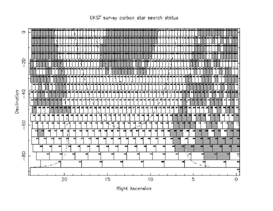
Figure 1: The southern UK Schmidt Telescope photographic regions surveyed are indicated in grey. The dashed line marks the Galactic plane, while the dot-dashed lines mark $b=30^{\circ}$ and $b=-30^{\circ}$.

Figure 6: Total Galactic rotation curves for the H1 (solid line) and H2 (dotted line) Halo mass models. In this diagram, the Halo mass has been normalized to give rise to a circular velocity of $v_{c}=220{\rm\,km\,s^{-1}}$ at $R=50{\rm\,kpc}$.

Figure 11: The relative likelihoods of the Galactic models are displayed, as a function of Halo mass flattening $q_{m}$, for the different combinations of Milky Way mass model (M1, M2) and dwarf galaxy model (D1, D2). In each panel, the solid line corresponds to $v_{c}(50{\rm\,kpc})=200{\rm\,km\,s^{-1}}$, the dashed line to $v_{c}(50{\rm\,kpc})=220{\rm\,km\,s^{-1}}$, and the dot-dashed line to $v_{c}(50{\rm\,kpc})=240{\rm\,km\,s^{-1}}$. The highest likelihood model is the more massive and extended D2 dwarf galaxy model simulated in the H2 (NFW-type) Galactic mass model with a spherical Halo. The preferred value of the circular velocity parameter is always $v_{c}(50{\rm\,kpc})=200{\rm\,km\,s^{-1}}$, while the preferred shape is always nearly spherical.

Figure 12: The difference between input and recovered Halo mass flattening $q_{m}$ as a function of input mass flattening, for the Monte Carlo tests described in §6.5.1. The cross, circle and square graph marker symbols show the mean flattening difference for the simulations in which the input circular velocity was, respectively, $v_{c}=200{\rm\,km\,s^{-1}}$, $v_{c}=220{\rm\,km\,s^{-1}}$ and $v_{c}=240{\rm\,km\,s^{-1}}$. (The input values of $q_{m}$ on the abscissa are shifted slightly to allow visualization).

Figure 13: Same as Figure 12, but for the test described in §6.5.3.

References

- Alcock et al. (1997) Alcock, C., et al. 1997, Astrophys. J. 486, 697
- Amendt & Cuddleford (1994) Amendt, P. & Cuddleford, P. 1994, Astrophys. J. 435, 93
- Azzopardi et al. (1998) Azzopardi, M., Breysacher, J., Muratorio, G. & Westerlund, B. E., 1998 in IAU Symposium 192 - The Stellar Content of Local Group Galaxies, eds. P. Whitelock and R. Cannon
- Becquaert & Combes (1997) Becquaert, J.-F., Combes, F. 1997, A&A 325, 41
- Binney, May & Ostriker (1987) Binney, J., May, A. & Ostriker, J. P. 1987, Mon. Not. R. astr. Soc. 226, 149
- Binney & Tremaine (1987) Binney, J. & Tremaine, S. 1987, Galactic Dynamics, Princeton University Press, Princeton
- Combes & Pfenniger (1997) Combes, F., Pfenniger, D. 1997, A&A 327, 453
- Cseresnjes, Alard & Guibert (2000) Cseresnjes, P., Alard, C., Guibert, J. 2000, astro-ph/0002157
- Dehnen & Binney (1998) Dehnen, W. & Binney, J. 1998, Mon. Not. R. astr. Soc. 294, 429
- Dubinski & Carlberg (1991) Dubinski, J. & Carlberg, R. 1991, Astrophys. J. 378, 496
- Dubinski (1994) Dubinski, J. 1994, Astrophys. J. 431, 617
- Evans (1994) Evans, N. W. 1994, Mon. Not. R. astr. Soc. 267, 333
- Evans & Jijina (1995) Evans, N. W. & Jijina, J. 1995, Mon. Not. R. astr. Soc. 267, L21
- Fahlman et al. (1996) Fahlman, G., Mandushev, G., Richer, H., Thompson, I. & Sivaramakrishnan, A. 1996, Astrophys. J. 459L, 65
- Fischer et al. (1999) Fischer, P., et al. 1999, astro-ph/9912119
- Gómez-Flechoso, Fux & Martinet (1999) Gómez-Flechoso, M., Fux, R., Martinet, L. 1999, A&A 347, 77
- Helmi & White (2000) Helmi, A., White, S. 2000, astro-ph/0002482
- Ibata, Gilmore & Irwin (1994) Ibata, R., Gilmore, G. & Irwin, M. 1994, Nature 370, 194
- Ibata et al. (1997) Ibata, R., Wyse, R., Gilmore, G., Irwin, M. & Suntzeff, N. 1997, Astr. J. 113, 634
- Ibata & Lewis (1998) Ibata, R., Lewis, G. 1998, Astrophys. J. 500, 575
- Ibata & Razoumov (1998) Ibata, R. & Razoumov, A. 1998, A&A 336 130
- Ibata et al. (2000a) Ibata, R., Gilmore, G., Irwin, M., Lewis, G., Wyse, R., Suntzeff, N. 2000, in preparation
- Ibata et al. (2000b) Ibata, R., Irwin, M., Lewis, G., Stolte, A. 2000, astro-ph/0004255
- Ibata et al. (2000c) Ibata, R., Lewis, G., Irwin, M. 2000, in preparation
- Irwin & Hatzidimitriou (1995) Irwin, M. & Hatzidimitriou, D. 1995, Mon. Not. R. astr. Soc. 277, 1354
- Irwin et al. (1996) Irwin, M., Ibata, R., Gilmore, G., Suntzeff, N. & Wyse, R. 1996, in: ‘Formation of the Galactic Halo’, ed A. Sarajedini, A.S.P., San Francisco
- Irwin & Totten (2000) Irwin, M. J. & Totten, E. 2000, in preparation
- Ivezic et al. (2000) Ivezic, Z., et al. 2000, Astr. J. 120, 963
- Jiang & Binney (1999) Jiang, I.-G., Binney, J. 1999, astro-ph/9908025
- Johnston, Spergel & Hernquist (1995) Johnston, K. V., Spergel, D. N. & Hernquist, L. 1995, Astrophys. J. 451, 598
- Johnston, Hernquist & Bolte (1996) Johnstone, K. V., Hernquist, L., Bolte, M. 1996, Astrophys. J. 465, 278
- Johnston et al. (1999) Johnston, K., Majewski, S., Siegel, M., Reid, I., & Kunkel, W. 1999, Astr. J. 118, 1719
- Katz (1991) Katz, N. 1991, Astrophys. J. 368, 325
- Katz & Gunn (1991) Katz, N. & Gunn, J. 1991, Astrophys. J. 377, 365
- Kuijken & Dubinski (1994) Kuijken, K. & Dubinski, J. 1994, Mon. Not. R. astr. Soc. 269, 13
- King (1962) King I. 1962, Astr. J. 67, 471
- Kunkel, Demers & Irwin (1997) Kunkel, W.E, Demers, S.D., & Irwin, M.J., 1997, A&AS 122, 463
- Lin et al. (1999) Lin, D., Jones, B., Klemola, A. 1995, Astrophys. J. 439, 652
- Lynden-Bell & Lynden-Bell (1995) Lynden-Bell, D. & Lynden-Bell R., M. 1995, Mon. Not. R. astr. Soc. 275, 429
- van der Marel (1991) van der Marel, R. P. 1991, Mon. Not. R. astr. Soc. 248, 515
- Moore et. al (1999) Moore, B, Ghigna, S., Governato, F., Lake, G., Quinn, T., Stadel, J., Tozzi, P. 1999, Astrophys. J. 524, 19L
- Morrison Flynn & Freeman (1990) Morrison, H., Flynn, C. & Freeman, K. C. 1990, Astr. J. 100, 1191
- Morrison et al. (2000) Morrison, H., Mateo, M., Olszewski, E., Harding, P., Dohm-Palmer, R., Freeman, K., Norris, J., Morita, M. 2000, astro-ph/0001492
- Navarro, Frenk & White (1997) Navarro, J., Frenk, C., White, S. 1997, Astrophys. J. 490, 493
- Oh, Lin & Aarseth (1995) Oh, K.S., Lin, D.N. & Aarseth, S.J. 1995, Astrophys. J. 442, 142