Abstract

Large-scale astrophysical systems are non-extensive due to their long-range force of gravity. Here we show an approach toward the statistical mechanics of such self-gravitating systems (SGS). This is a generalization of the standard statistical mechanics based on the new definition of entropy; Tsallis statistical mechanics. Developing the composition of entropy and the generalized Euler relation, we investigate the galaxy distributions in count-in-cell method. This is applied to the data of CfA II South redshift survey.

1 Introduction

Astrophysical systems in the Universe are characterized by the gravitation. The structure formed through this long-range force is quite different from those formed through the other short-range forces. If the system does not strongly depend on the initial conditions of the Universe, we can apply statistical mechanics for describing such self-gravitating systems (SGS). However, we cannot directly apply the standard Boltzmann statistical mechanics for SGS since the long-range nature of gravity strongly violates the extensive property of the system which is the premise of statistical mechanics. Actually, the total energy increases much faster than the particle number $N$, the partition function $Z$ often becomes complex[1], reflecting the fact that there is no absolute stable state in SGS.

In order to seek for workable statistical mechanics of SGS, we try an approach based on the new definition of entropy whose extensivity is violated from the beginning; Tsallis statistical mechanics.

We formulate the count-in-cell method for the large scale galaxy distributions in this new statistical mechanics. First we calculate the expression of the composite entropy and the generalized Euler relation in this new statistical mechanics. These are applied to the data of CfA II South redshift survey. The parameter q becomes negative, which represents the instability of gravity.

2 Tsallis Statistical Mechanics

The ordinary Boltzmann statistical mechanics is characterized by the entropy $S=-\sum\limits_{i}{p_{i}\ln p_{i}}$. The distribution function $p_{N,E}=\exp\left[{-\left({E-\mu N}\right)/T}\right]/\Xi$ maximizes this entropy with constraints of the probability conservation, the energy conservation, and the particle number conservation. This statistical mechanics is originally aimed to describe the multi-fractal and chaos structures. It is characterized by the entropy of the form [2] $S_{q}\left[p\right]=\left({\sum\limits_{i}{p_{i}^{q}-1}}\right)/(1-q)$, where $q$ is a real parameter. Tsallis distribution function is obtained so that it maximizes this entropy with the same constraints. The solution has a power law tail:

$$p_{N,E}=\frac{1}{{\Xi_{q}}}\left\{{1-\frac{{1-q}}{{\tilde{T}}}\left({E-\bar{E}-\mu\left({N-\bar{N}}\right)}\right)}\right\}^{\frac{1}{{1-q}}},$$ (1)

where $\tilde{T}\equiv CT$, and $C=\sum\limits_{i}{p_{i}^{q}}$. Partition function is defined as

$$\Xi_{q}=\sum\limits_{N,E}{\left\{{1-\frac{{1-q}}{{\tilde{T}}}\left({E-\bar{E}-\mu\left({N-\bar{N}}\right)}\right)}\right\}^{\frac{1}{{1-q}}}}.$$ (2)

Note that $p_{N,E}$ reduces to the ordinary Boltzmann form for $q\to 1$. For the consistent formulation, it is important to notice that the observable expectation value is calculated by the escort distribution[3]: $P_{i}=p_{i}^{q}/C$, $\left\langle Q\right\rangle_{q}=\sum\limits_{i}{P_{i}Q_{i}}$. The averaged quantities $\bar{E},\bar{N}$ in Eqs.(1) and (2) should be understood in this sense.

3 Galaxy Distribution in Count-in-Cell Method

There are many approaches to describe large scale structure of the Universe. In this paper, we will concentrate on distribution of galaxies. One of the well-known method to describe the distribution of galaxies is the two-point correlation function. However, when we solve equations of motions for the two-point correlation function, we need three-point correlation function. Such higher order essentialness is called BBGKY chain. Since we have to cut the BBGKY chain, we have to apply some kind of approximations.

On the other hand, count-in-cell method is often used to describe distribution of galaxies. In this method, we use an analytic formula for probability $f(N)$ of finding $N$ galaxies in a randomly positioned volume $V$. As we don’t have to use any approximation in count-in-cell method, we can apply it even for clustered system. Saslaw and Hamilton[4], and S. Inagaki introduced the virial parameter b=(gravitational correlation energy)/(kinetic energy of random motion), which measures the deviation from the dynamical-equilibrium. Then they found that in thermal-equilibrium, their theoretical investigation of $f(N)$ is consistent with he N-body simulations or catalogues of observations. Strictly speaking, we should not apply thermal-equilibrium theory for expanding Universe. However their consistency let us further study thermal-equilibrium statistical description. In evolution of the Universe, dynamical-equilibrium $b=1$ must be realized before the Universe reach thermal-equilibrium. Therefore in this paper we consider the dynamical-equilibrium $b=1$ case. We believe that there exist adequate fitting parameter other than the virial parameter $b$. That is the reason why we consider non-extensive statistics which gives us parameter $q$.

Supposing the galaxies distribute according to Tsallis statistics, we consider a system described by equilibrium thermodynamics. That is the grand canonical ensemble, characterized by the given temperature and the chemical potential.

The probability to find no galaxy in the volume $V$ is

$$f\left(0\right)\equiv\sum\limits_{E}{P_{0,E}}=P_{0,0}=\frac{{\left({p_{0,0}}\right)^{q}}}{C},$$ (3)

where

$$p_{0,0}=\Xi_{q}^{-1}\left[{1+\frac{{1-q}}{{\tilde{T}}}\left({\bar{E}-\mu\bar{N}}\right)}\right]^{\frac{1}{{1-q}}}.$$ (4)

The partition function can be decomposed as

$$\Xi_{q}=\sum\limits_{N,E}{\left({1-\frac{{1-q}}{{\tilde{T}}}\left({E-\bar{E}-\mu\left({N-\bar{N}}\right)}\right)}\right)^{1+q/\left({1-q}\right)}}=\left({\Xi_{q}}\right)^{q}C$$ (5)

and therefore $\Xi_{q}=C^{1/\left({1-q}\right)}=\left({1+\left({1-q}\right)S}\right)^{1/\left({1-q}\right)}$. Thus we obtain

$$f\left(0\right)=\left({1+\left({1-q}\right)S}\right)^{\frac{{-1}}{{1-q}}}\left({1+\frac{{1-q}}{{\tilde{T}}}\left({\bar{E}-\mu\bar{N}}\right)}\right)^{\frac{q}{{1-q}}}.$$ (6)

In order to reduce the above expression, we need to calculate the composite entropy and the Euler relation in Tsallis statistics. When we compose two systems A and B, the distribution function is given by $p_{ij}(A,B)=p_{i}(A)p_{j}(B)$ and the composed entropy is $S_{A+B}=S_{A}+S_{B}+\left({1-q}\right)S_{A}S_{B}.$ Sequentially using this composition $S_{N+1}=s+S_{N}+\left({1-q}\right)sS_{N}$, (where $s$ means entropy of 1 system), we obtain the total entropy of N identical systems as

$$S_{N}=\frac{{\left({1+\left({1-q}\right)s}\right)^{N}-1}}{{1-q}}.$$ (7)

Generalized Euler relation is given by the following arguments. The variables $E,V,N$ are the natural arguments of the entropy: $S_{N}=S\left({E,V,N}\right)$. Differenciating $S_{\alpha N}=S\left({\alpha E,\alpha V,\alpha N}\right)$ with respect to $\alpha$ and setting $\alpha\to 1$, we obtain

$$\left.{\frac{{\partial S_{\alpha N}}}{{\partial\alpha}}}\right|_{\alpha\to 1}=\left.{\frac{{\partial S\left({\alpha E,\alpha V,\alpha N}\right)}}{{\partial\alpha}}}\right|_{\alpha\to 1}=\frac{E}{T}+\frac{{pV}}{T}-\frac{{\mu N}}{T},$$ (8)

where we used $\partial S/\partial V=p/T,\;\partial S/\partial E=1/T,\;\partial S/\partial N=-\mu/T$, which are guaranteed by the Legendre structure of the Tsallis thermodynamics[5]. In the above, we can put any other values for $\alpha$ as well. In general, the $\alpha$-dependence is inherited from $S$ to $T$ on the right hand side of Eq.(8). Non-extensivity of $S$ necessarily accompanies the non-intensivity of the Legendre-conjugate variable $T$. Actually, the fact that the variables $E,V,N$ are extensive and $p,\mu$ are intensive in Eq.(8) renders the $\alpha$-dependence of the temperature:

$$T\left(\alpha\right)=T_{1}\left({1+\left({1-q}\right)s}\right)^{1-\alpha N}$$ (9)

where $T_{1}$ is the temperature of one particle system. Note that $\tilde{T}\equiv CT$ defined just after Eq.(1) is $\alpha$-independent! Probably this quantity $\tilde{T}$ should be related with the physical temperature as defined from the velocity dispersion of the system. However at present, we do not have idea on the meaning of the quantity $T$. This point will be further discussed in the last section.

Then we obtain the Euler relation in non-extensive statistical mechanics

$$\frac{{\left({1+\left({1-q}\right)S}\right)\ln\left[{1+\left({1-q}\right)S}\right]}}{{1-q}}=\frac{{E+pV-\mu N}}{T}.$$ (10)

This temperature on the right hand side is $T\left({\alpha=1}\right)$ in Eq.(9), though the explicit form of the temperature does not appear in the final expression of $f\left(N\right)$. Using this Euler relation, we can now eliminate $\bar{E}-\mu\bar{N}$ in $f\left(0\right)$ and Eq.(6) reduces to

$$f\left(0\right)=\left({1+\left({1-q}\right)S}\right)^{\frac{{-1}}{{1-q}}}\left({1-\frac{{pV}}{{\tilde{T}}}\left({1-q}\right)+\ln\left[{\left({1+\left({1-q}\right)S}\right)}\right]}\right)^{\frac{q}{{1-q}}}.$$ (11)

Since we consider the dynamical-equilibrium system, the system is fully virialized $b=1$, and therefore the pressure $p$ must be $0$, we obtain:

$$f\left(0\right)=\left({1+\left({1-q}\right)S}\right)^{\frac{{-1}}{{1-q}}}\left({1+\ln\left[{\left({1+\left({1-q}\right)S}\right)}\right]}\right)^{\frac{q}{{1-q}}}.$$ (12)

Moreover using Eq.(7), we finally obtain

$$f(0)=\left\{{1+\left({1-q}\right)s}\right\}^{\frac{{-N}}{{1-q}}}\left[{1+N\ln\left\{{1+\left({1-q}\right)s}\right\}}\right]^{\frac{q}{{1-q}}}.$$ (13)

Our parameters are $s$ (the unit of non-extensive entropy per galaxy) and $q$ (the Tsallis statistical parameter).

Probability of finding $N$ galaxies in the volume V is generated from $f\left(0\right)$:

$$f\left(N\right)\equiv\frac{{(-n)^{N}}}{{N!}}\frac{{d^{N}}}{{dn^{N}}}f(0)$$ (14)

where $n$ is the galaxy number density[6]. This is because the void probability $f\left(0\right)$ contains all the information of the whole correlation functions:

$$f\left(0\right)=1-\int{P\left\{{X_{1}}\right\}}+\int{\int{P\left\{{X_{1}X_{2}}\right\}}}-\int{\int{\int{P\left\{{X_{1}X_{2}X_{3}}\right\}}}}\pm\cdots,$$ (15)

where $P\left\{{X_{1}X_{2}}\right\}$ is the probability that there are galaxies in $dV_{1}$ at $X_{1}$ and $dV_{2}$ at $X_{2}$. The above expression guarantees that the probability is properly normalized: $\sum\limits_{N=0}^{\infty}{f\left(N\right)}=1$.

4 Comparison with observations

We use the data of CfA II South redshift observations which includes 4392 galaxies [7]. We have to reduce the data to the uniform sample. First we restrict the data to the galaxies whose absolute luminosity is brighter than the magnitude -19.1 and the distance $4,000\sim 8,000[{{\rm km}/\sec}]$. The distance is measured by the cosmic redshift. We further exclude the edge of the observation region. We applied the K-correction for compensating the reddening. Finally the data is reduced to 870 galaxies. The number density is $n=4.44\times 10^{-9}[\left({{\rm km}/\sec}\right)^{-3}]$.

We first fit the void probability $f\left(0\right)$ by varying the parameters q and s. The best fit is realized by $q=-5.66847{\rm}$ and $s=0.164142{\rm}$ (Fig.1). We fix these values and do not change them hereafter in this paper. With these parameters, general probability $f\left(N\right)$ is given. In Figs.1-2, we compared our calculations and the CfA data.

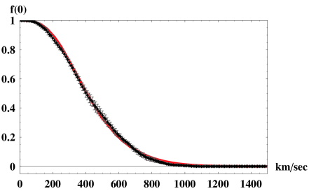
Figure 1: The void probability $f\left(0\right)$. CfA II South Observations (dots with error bars) and our calculations (Solid lines) are plotted. From this fit, we obtained the parameters q and s, which should be kept unchanged hereafter.

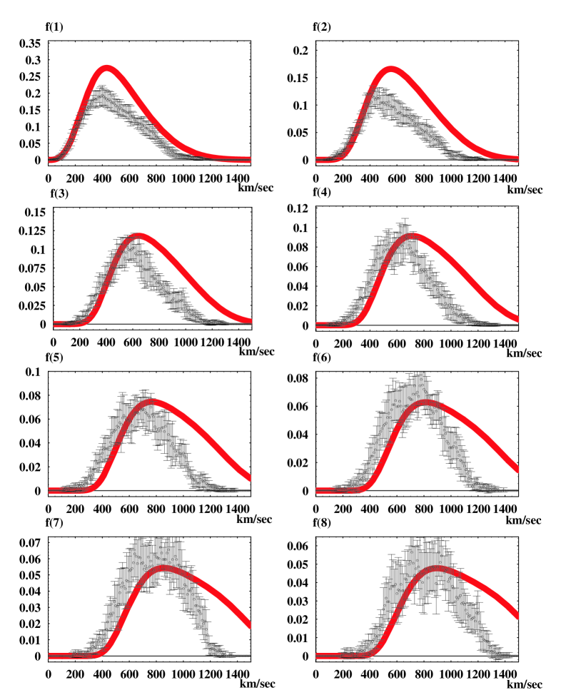
Figure 2: Probability functions $f\left(1\right)$ through $f\left(8\right)$, from left to right and top to bottom. CfA II South Observations (dots with error bars) and our calculations (Solid lines) are plotted.

We have checked the normalization of probabilities $\sum\limits_{N=0}^{\infty}{f\left(N\right)}=1$ is realized.

The negative value of $q$ we obtained may not be so surprising. In reference [8], the value of $q$ appears to decrease monotonically from 1 to $-\infty$ for one-dimensional logistic maps. Their model reveals unstable onset-to-chaos attractor. For negative $q$, the entropy functional loses its convexity and the distribution becomes unstable. Thus the intrinsic instability of SGS is faithfully represented in this formalism and this fit.

5 Conclusions and Discussions

We have constructed the non-extensive statistical mechanics based on the non-extensive entropy. Especially calculating the entropy of composite systems and deriving the generalized Euler relation in thermodynamics, we could evaluate the void probability function $f\left(0\right)$ and the probability to find $N$ galaxies $f\left(N\right)$. This result was applied to the CfAII South galaxy observations and we have obtained negative parameter $q$. This is thought to be another representation of the intrinsic instability of SGS. It will be also interesting to notice the fact that the multi-fractal scaling is observed in this CfAII South data within the scale-region from $500[{\rm km/sec}]$ to $3000[{\rm km/sec}]$[9]. We would like to clarify possible connection between the non-extensive distributions and the multi-fractal nature in the context of gravity.

On the way we derive $f\left(N\right)$, we encountered “scale ($\alpha$) dependent temperature $T$”. If we put the values we obtained $q=-5.66847{\rm}$ and $s=0.164142{\rm}$ to Eq.(9), we can explicitly plot the scale dependence of the temperature. It turns out to reduce with increasing scale and abruptly drops to zero at about $r\approx 600[{\rm km/sec}]$ or, assuming the cosmic expansion speed as $H=72[{\rm km/sec/Mpc]}$, at about $8.3[{\rm Mpc}]$, which is almost the scale that the galaxy correlation function becomes unity. On the other hand, it is apparent that the galaxies do have peculiar velocity of order $1000[{\rm km/sec}]$ at this scale. Therefore, at least, the quantity $T$ cannot be interpreted as the ordinary temperature as defined from the velocity dispersions. One of our next task will be to elucidate the meaning of $T$.

In relation with the astronomical velocity distributions, the authors[10] claim that the velocity distribution of the clusters of galaxies can be well fitted by the Tsallis distribution with the parameter $q=0.23_{-0.05}^{+0.07}$, which is apparently different from our negative value for galaxy distributions. Further study on the velocity distributions in various scales (galaxies, clusters, super-clusters) would reveal the origin and evolution of the large-scale structure of Universe. We would like to report these results in the near future.

References

- [1] O. Iguchi, T. Kurokawa, M. Morikawa, A. Nakamichi, Y., T. Tatekawa, and K-I Maeda, Phys. Lett. A 260, 4 (1999).
-
[2]
C. Tsallis, J. Stat. Phys 52, 479 (1988).
C. Tsallis, Braz. J. Phys. 29, 1 (1999) (cond-mat/9903356) for a review. http://tsallis.cat.cbpf.br/biblio.htm for a comprehensive reference. - [3] C. Tsallis, R.S. Mendes and A.R. Plastino, Physica A 261, 534 (1998).
- [4] W. C. Saslaw and A. J. S. Hamilton, ApJ 276, 13 (1984).
- [5] A. Plastino and A. R. Plastino, Phys. Lett. A226 257 (1997).
- [6] S. D. M. White, MNRAS 186, 145 (1979).
- [7] J. Huchra, et al., ApJS in press (CfA preprint 4486) (1998).
- [8] U. M. S. Costa, M. L. Lyra, A. R. Plastino and C. Tsallis, Phys. Rev. E56, 245 (1997).
- [9] T. Kurokawa, M. Morikawa, H. Mouri, A&A 344, 1 (1999).
-
[10]
A. Lavagno, G. Kaniadakis, M. Rego-Monteiro, P. Quarati, and C. Tsallis,
Astro. Lett. and Communications 35, 449 (1998).