Simulated Submillimetre Galaxy Surveys

Abstract

Current submillimetre surveys are hindered in their ability to reveal detailed information on the epoch of galaxy formation and the evolutionary history of a high-redshift starburst galaxy population. The difficulties are due to the small primary apertures ($\rm{D<15}$-m) of existing submillimetre telescopes and the limited sensitivities of their first generation of bolometer cameras. This situation is changing rapidly due to a variety of powerful new ground-based, airborne and satellite FIR to millimetre wavelength facilities. Improving our understanding of the luminosity and clustering evolution provides the motivation for conducting cosmological submillimetre and millimetre surveys. It is therefore important that we quantify the limitations of the future surveys and the significance of the results that can be drawn from them. In this paper we present simulated surveys which are made as realistic as possible in order to address some key issues confronting existing and forthcoming surveys. We discuss the results from simulations with a range of wavelengths (200$\mu$m – 1.1 mm), spatial resolutions (6– 27) and flux densities (0.01–310 mJy). We address how the measured source-counts could be affected by resolution and confusion, by the survey sensitivity and noise, and by the sampling variance due to clustering and shot-noise.

1 Introduction

By early 2001 the initial extensive programme of extragalactic SCUBA (850$\mu$m) surveys conducted on the 15-m JCMT will be completed. The targets of these sub-mm surveys include lensing clusters (Smail et al. 1997), the Hubble Deep Field (Hughes et al. 1998), the Hawaii Deep Survey fields (Barger et al. 1998, 1999), the Canada-France Redshift Survey fields (Eales et al. 1999, Lilly et al. 1999) and the UK 8 mJy SCUBA surveys of the ISOPHOT ELAIS and Lockman Hole field (in prep.) These blank-field sub-mm surveys, which cover areas of $\sim 0.002-0.2$ deg², allow a measure of the $850\mu$m source-counts between flux densities of 1–15mJy. The relatively small survey areas are due to the low mapping speed (a combination of the field-of-view and sensitivity of the bolometer array, and the necessary overheads to fully sample the focal-plane with $\rm>0.5F\lambda$ feedhorns, e.g. 16 separate secondary-mirror positions are required to fully sample the SCUBA array). The restricted 850$\mu$m flux range in the measured source-counts is the result of a source-confusion limit of $\sim 2$ mJy (due to a small primary aperture or map resolution) at faint flux densities and the small survey area at the bright end, given the intrinsic low source-density of bright sub-mm sources (e.g. $N[S_{850_{\mu m}}>20\rm\,mJy]<70~{}~{}sources/deg^{2}$).

The limitations on the accuracy of our understanding of high-z galaxy evolution from sub-mm surveys has been described elsewhere (Hughes 2000). To improve the constraints on the competing evolutionary models, future sub-mm and mm surveys must extend their wavelength coverage, increase their survey area and sensitivity. To quantify the advantages of these forthcoming surveys we have simulated the extra-galactic sky at various sub-mm and mm wavelengths (200-3000$\mu$m), spatial resolutions ($\theta_{FWHM}\sim 1-120$) and sensitivities ($S>0.01$ mJy). We include in the simulations contributions from CMB primary fluctuations, S-Z clusters, an evolving extra-galactic population of star-burst galaxies and high-latitude galactic-plane cirrus emission. These simulated surveys allow us to compare the measured source-counts for a wide variety of current and future FIR and sub-mm/mm telescopes (e.g. SIRTF, FIRST, MAP, PLANCK, BLAST, SOFIA, CSO, JCMT, LMT, GBT, ALMA).

We discuss these multi-wavelength simulations in more detail elsewhere (Hughes & Gaztañaga 2000). In this paper we concentrate on illustrating the effects of galaxy clustering and low spatial resolution on the measured source-counts at 1100$\mu$m, 850$\mu$m, 350$\mu$m and 200$\mu$m.

2 Simulations

The starting point for our simulations is a $P^{3}M$ N-body simulation with $200^{3}$ particles in a $600h^{-1}{\rm Mpc}$ box that has the same matter power spectrum as that measured for APM Survey galaxies (see Gaztañaga & Baugh 1998, and references therein). Thus, the 2-point correlation in the (dark) matter particles is identical to the one measured in the local ($\bar{z}\simeq 0.15$) galaxy universe. Using a single N-body output (as opposed to a light-cone output) corresponds to having the matter clustering pattern fixed in comoving coordinates (stable clustering). If redshift evolution of the two-point correlation function $\xi_{2}(r,z)$ is parametrized as:

$$\xi_{2}(r,z)=(1+z)^{-(\epsilon+3)}~{}\xi_{2}(r),$$ (1)

then, for stable clustering we have $\epsilon\simeq 0$ at small scales (e.g. see Gaztañaga 1995). This has less clustering evolution than pure matter gravitational clustering (e.g. linear or non-linear growth, where $\epsilon\simeq 1$) and might describe some models in which galaxies are identified with high-density matter peaks (peaks move less than particles, which results in less evolution). This might be adequate for star-forming galaxies if we are selecting rarer (more massive) objects as we go to higher redshifts. It is in agreement with the strong clustering observed in Lyman-break galaxies at $z\simeq 3$, which is comparable to the clustering of present-day galaxies (see Giavalisco et al.  1998).

We next implement a model for the evolution of the galaxy population and set the geometry of a light-cone observation. To relate spatial coordinates $r$ and observed redshifts $z$ in the simulation output we use a spatially flat metric with the critical density $\Omega=1$ and zero cosmological constant (other cosmological parameters will be considered elsewhere). We transform the N-body matter simulation into a mock galaxy catalogue of angular and redshift positions by the following steps:

• i) select an arbitrary point in the simulated box to be the local ‘observer’;

• ii) apply a given survey angular mask (e.g. a square with 1 degree on a side);

• iii) include in the mock catalogue a simulated particle at redshift $z$ from the observer with probability given by some selection function $\psi(z)$;

• iv) assign a luminosity $L=L(\lambda)$ to this particle according to the luminosity function $\phi[L,z]$ for each one of the observer filters $\lambda$, at the corresponding particle redshift $z$.

We replicate the N-body (periodic) simulation box to cover the total extent of the survey (up to $z=6$, beyond which we impose an exponential cut-off in the expected number of galaxies). By comparing the results from different box sizes we have verified that this replication of the box does not introduce any spurious correlations on large scales. The selection function $\psi(z)$ is the normalized probability that a galaxy at redshift $z$ is included in the catalogue, and is proportional to the estimated number of galaxies at this coordinate:

$$\psi(z)\propto\int_{L_{1}(z)}^{L_{2}(z)}~{}dL~{}\phi[L,z].$$ (2)

where $\phi[L,z]$ is the luminosity function and $L_{1}(z)$ and $L_{2}(z)$ are the luminosities corresponding to the lower and upper limits in the range of apparent fluxes used to build the galaxy sample or catalog under study. Thus our prescription for galaxy formation is that, on average, the probability to find a galaxy is simply proportional to the (dark) matter densities, so that the number density of galaxies automatically determines how massive are the matter peaks that our galaxies are tracing. Other “biasing” schemes can also be implemented, but note that different models for galaxy formation can give different clustering evolutions for a given $\phi[L,z]$, so that both of these evolutionary patterns need to be better constrained by the future data if we want more realistic simulations.

To include the star-formation history of the galaxies in our simulations we have selected models describing the SEDs shown in Figure 1 to extrapolate the local IRAS $60\mu$m local luminosity function $\phi[L,z=0]=\phi[L/L^{*}]$ (Saunders et al. 1990) to longer wavelengths. We have introduced an exponential cutoff for objects fainter than $L=10^{8}L_{\odot}$ and adopted a model of pure luminosity evolution, $\phi[L,z]=\phi[L/L^{*}]$, with the following redshift dependence: $L^{*}(z)=(1+z)^{3}~{}L^{*}(z=0)$ for $0<z<2.2$; $L^{*}(z)=L^{*}(z=2.2)$ for $2.2\leq z<6$; an exponential cutoff at $z>6$.

In this paper we use a single SED model of Arp220 for all galaxies in our sample. As will be shown below (Figure 4), using a different SED makes no significant difference in the number counts or redshift distributions even for bright sources at the shortest submillimetre wavelengths. We have also assumed no evolution for the SED: if the evolution occurs within the spread in the models shown in Figure 1, this has little effect for $\lambda\simeq 200-1100\mu$m.

Figure 1: Radio to IR SEDs of low-z starbursts, quasars, ULIRGS, Seyferts normalised at 60$\mu$m. The curves represent fits to the SEDs of Arp220 (solid), M82 (dashed) and Mkn231 (dashed-dotted). Since the rest-frame SEDs show a large dispersion in the spectral slope at $\lambda<60\mu$m then only the number-counts of the highest-z sources ($z>3$) in the shortest wavelength simulations (200-300$\mu$m) are sensitive to the exact choice of galaxy SED type or its redshift evolution.

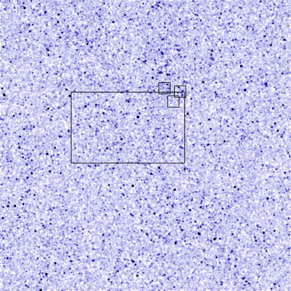
Figure 2: A confusion-limited ($1\sigma=0.5$ mJy) JCMT 1 deg² area simulated survey at 850$\mu$m with $\theta_{FWHM}=15$. The large and small boxes show the 0.1 deg² area and the HDF-like regions shown in Figures 3 & 8 respectively.

	LMT Surveys	NEFD = 10 mJy sec1/2 , $\eta\sim 100\mu$m		NEFD = 4 mJy sec1/2 , $\eta\sim 70\mu$m
Survey	Area (sq. arcmins)	3-$\sigma$ depth	N ($5-\sigma$ galaxies)	3-$\sigma$ depth	N (5-$\sigma$ galaxies)
A	6	0.1 mJy	18	0.05 mJy	33
B	350	0.9 mJy	204	0.4 mJy	515
C	1000	1.6 mJy	320	0.6 mJy	1100
D	3600	3.0 mJy	400	1.2 mJy	1600

Table 1: Number of 5-$\sigma$ galaxies detected in alternative 50-hour BOLOCAM 1.1 mm surveys with a conservative Noise Equivalent Flux Density (NEFD) of NEFD = 10 mJy sec^1/2 at 1.1 mm, during the initial commissioning phase (e.g. with a primary aperture r.m.s. surface accuracy of $\eta\simeq 100\mu$m r.m.s.) of the LMT; and later during routine operation with an improved surface accuracy (of $\eta\simeq 70\mu$m) and 1.1 mm NEFD = 4 mJy sec^1/2. BOLOCAM sensitivities allow for overheads. Surveys A and B represent LMT surveys similar in area to the SCUBA survey of the HDF and the UK 8 mJy wide-area survey respectively. Surveys C and D represent future wide-area LMT surveys.

 

 

 

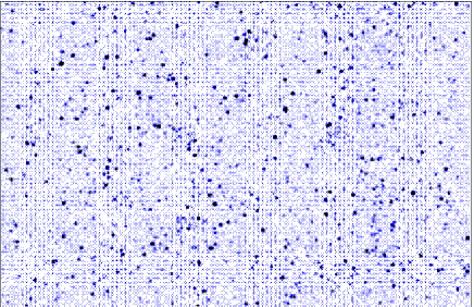
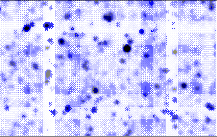
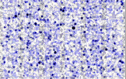
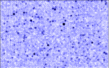
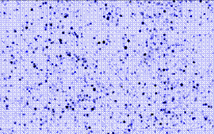
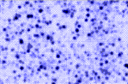
Figure 3: Simulated surveys covering 0.1 deg²: A confusion-limited ($3\sigma=0.05$ mJy) LMT survey at 1100$\mu$m with $\theta_{FWHM}=6$(top-left); a $\theta_{FWHM}=27$low resolution 1100$\mu$m survey (top-right); a $\theta_{FWHM}=15$deep ($1\sigma=0.5$ mJy) 850$\mu$m survey (middle-left); a $\theta_{FWHM}=15$shallow ($1\sigma=2.5$ mJy) 850$\mu$m survey (middle-right); a confusion-limited ($\theta_{FWHM}=9$) 350$\mu$m survey (bottom-left); a confusion-limited ($\theta_{FWHM}=25$) 200$\mu$m survey (bottom-right). These figures look much better in http://www.inaoep.mx/ gazta/simsubmm.ps

Thus, after these transformations we end up with a galaxy catalogue of angular positions, redshifts and luminosities, for each of the observer filters $\lambda$. We next smooth the resulting projected distribution with a spatial resolution appropriate to the observational configuration we are simulating: $\theta_{FWHM}\simeq 1.2~{}\lambda/\rm D$ where $\rm D$ is the telescope aperture. Finally we add white noise ${\cal N}$ to the angular catalogue to emulate the signal-to-noise ${\cal S/N}$ appropriate for the integration time, $t$, the instrumental sensitivity and observational conditions (Noise Equivalent Flux Density, NEFD) of the mock survey we want to emulate.

We describe here the results from simulated surveys at 1.1 mm, 850$\mu$m, 350$\mu$m and 200$\mu$m with spatial resolutions of 6, 15, 9and 25corresponding to surveys on the 50-m LMT (http://binizaa.inaoep.mx), 15-m JCMT, 10-m CSO and 2-m BLAST (http://www.hep.upenn.edu/blast/) respectively. The full simulations have a flux dynamic range of $S_{\lambda}=0.01-310$ mJy at all wavelengths and cover an area of 1 sq. degree. Subsets have been extracted to determine the source-counts from surveys comparable in area (6–400 arcmin², Table 1 - survey A and B) to the SCUBA surveys of the Hubble Deep Field and Hawaii Deep Fields, the lensing cluster survey, Canada-France Redshift survey fields and the UK 8 mJy ELAIS and Lockman Hole survey. Additionally larger-area surveys (0.3–1.0 deg², Table 1 - surveys C and D) more appropriate to the LMT and BLAST are also considered.

Figure 2 shows a large projected (1 deg²) map at 850$\mu$m with some identified sub-regions within which we perform the source-counts analysis. Although there is significant clustering in this figure, the overall distribution is already quite homogeneous. Figure 3 shows a comparison of maps at different resolutions and wavelengths from the 0.1 deg² region in the center of the larger map.

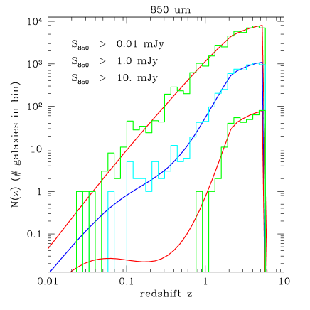
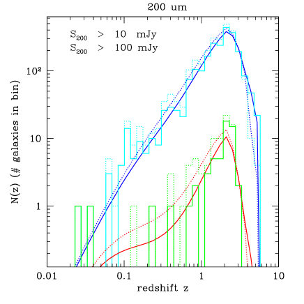
Figure 4: Redshift distribution, $N(z)$, of simulated sources (histograms) compared to input model (solid-lines). Left-panel shows $N(z)$ at 850$\mu$m for sources brighter than 0.01, 1.0, 10.0 mJy. Right-panel compares $N(z)$ at 200$\mu$m for sources brighter than 10 and 100 mJy: The dotted and continuous lines correspond to the use of Arp220 and M82 as the template to model the galaxy SED.

In general, one can recognise the brightest sources in an individual map at any other wavelength. Consequently it is possible to derive a robust constraint on the redshift of an individual galaxy from the relative intensities at different wavelengths (e.g. Hughes 2000). Nevertheless, even if we choose the sensitivity limits at each wavelength to have similar mean redshifts, the redshift distribution for the $200\mu$m galaxies is quite different from that of $850\mu$m (e.g. see Figure 4). Therefore care must be taken in determining the appropriate depths of the complementary surveys when the goal is to measure millimetre to submillimetre colours to estimate the redshift distribution. These redshift issues will be quantified in more detail elsewhere (Hughes & Gaztañaga 2000).

3 Source-Count Analysis

To demonstrate the simulations accurately reproduce the input models we show in Figure 4 the match between the expected number of galaxies at 850$\mu$m and 200$\mu$m in a given log redshift bin, $N(z)$, as given by the input selection function, and the measured counts in the redshift simulations (before including the noise or the finite resolution to the map). Figure 4 also shows a comparison of the results for the brighter counts using two different SEDs models: Arp220 and M82. As shown in Figure 1, the difference in the SED models is larger at $\lambda>60\mu$m, so that for mean redshifts of $z\simeq 2-3$, the choice and/or evolution of the galaxy SED will only affect the counts at the shortest sub-mm wavelengths (e.g. $300-200\mu$m). The right-hand panel of Figure 4 illustrates that at $200\mu$m the effects of using different SED models on the bright counts ($\sim 100$ mJy) are small. The results at fainter $200\mu$m fluxes or at other wavelengths are not shown as the differences in the histograms are indistinguishable for different SEDs. However the effect on the counts of the brightest $200\mu$m sources is also negligible compared to the sampling effects due to clustering discussed in §3.3.

The number counts and photometry of the sources in our simulated angular maps were determined using SEXTRACTOR (within the STARLINK package GAIA). In Figure 5 we compare the predicted and measured number-counts of the sources extracted from the full 1-deg² simulations at 1100, 850 and 200$\mu$m. Again there is excellent agreement between the simulated source-counts and the model down to the confusion flux limit of the different surveys at their respective resolutions. This illustrates the obvious point that provided the survey is of sufficient area and sensitivity then neither resolution, projection or noise are very important in extracting counts for objects above the confusion-limit.

3.1 Resolution and confusion

Below the confusion limit the counts flatten as faint sources merge to form brighter objects (see Figure 5). For example, at 850$\mu$m the counts are affected by confusion at $S_{850\mu m}\leq 2$ mJy, whilst at 1.1 mm with 6resolution (e.g. LMT) the counts are still unaffected at $S_{1.1\rm mm}\sim 0.1$ mJy. Even at lower resolution (27) the measured 1.1 mm source-counts recover the input model down to $S_{1.1\rm mm}\sim 3$ mJy due to the low density of intrinsically luminous sources ($>10^{12}L_{\sun}$). Similarly the 200$\mu$m counts recover the model down to a confusion limit of 18 mJy at 25resolution. Hence, even at resolutions of $\sim 30\arcsec$ the overlapping of individual source PSFs is negligible, regardless of whether it’s due to the random line-of-sight projection of galaxies at different redshifts, or because of a high-amplitude of clustering. The significance of this result is that it is therefore possible to combine large-aperture (50-m LMT, 15-m JCMT) 3000–450$\mu$m wavelength surveys and relatively small primary aperture (e.g. $\sim 2.0$ m BLAST) sub-mm and FIR surveys ($500-200\mu$m) with very different resolutions ($\theta_{FIR}/\theta_{\rm mm}\sim 5$) and still derive meaningful colours of sub-mm-selected galaxies, and hence constrain their redshifts (Hughes 2000).

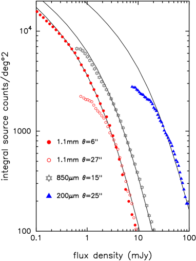
Figure 5: A comparison of the input model (solid-lines) and the extracted source-counts from the simulated 1-deg² surveys at 200$\mu$m, 850$\mu$m and 1.1 mm. Note how the simulated counts are depleted with respect to the input model at fluxes fainter than the confusion limit, which is set by the spatial resolution of the survey. The 1.1 mm counts at different resolutions (6and 27) are also shown.

3.1.1 Extra-galactic Background

The 1.1 mm extra-galactic background with flux $S>0.5$ mJy due to the discrete sources in our simulations is $1.31\times 10^{-10}\rm\,Wm^{-2}sr^{-1}$, in excellent agreement with FIRAS (Far Infrared Absolute Spectrophotometer) results from COBE residual measurement of the extra-galactic far infrared background (e.g. Dwek et al. 1998 and references therein). This implies that surveys conducted at the full spatial resolution of the LMT could resolve $\sim 100\%$ of the mm background, whilst the deepest SCUBA surveys todate have resolved only 30-50% of the sub-mm background.

3.2 Depth and noise

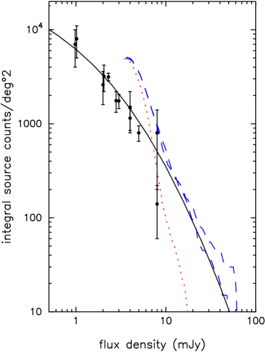
Figure 6: Extracted number-counts at 850$\mu$m from two (3$\sigma\sim 8$ mJy) 0.2 deg² simulated surveys (dashed-lines). The symbols show the actual observed SCUBA 850$\mu$m number-counts from the surveys described in §1 and the solid line correspond to the the model described in §2 (which is the input to the simulations). The counts from the noise map (1$\sigma=2.5$ mJy), which was added to the raw simulation, are shown as a dotted line. Because these are not deep surveys, the noise dominates the counts producing spurious simulated sources at 8-12 mJy. This has the opposite effect to the confusion produced by the finite resolution shown in Figure 5.

In the previous subsection we indicated that provided surveys have sufficient sensitivity that they can reach their confusion limit then accurate source-counts can be measured from large-area surveys. However the simulations also illustrate the way in which the counts are severely affected for shallow wide-area surveys with a flux-limit well above the confusion limit when the number-counts are steep. For example Figure 6 shows the simulated counts from a 0.2 deg² 850$\mu$m SCUBA survey with a 1-$\sigma$ sensitivity of 2.5 mJy. The extracted counts accurately reproduce the model down to a flux density of $\sim 12$ mJy, below which a steep increase in the counts is observed due entirely to the noisy background. Hence individual sources identified in shallow sub-mm surveys at the 3–5$\sigma$ level may be spurious. These additional sources can have a non-negligible positive contribution to the overall number counts (compared to the situation in §3.1 where the counts flatten at the confusion-limit of the survey). This is due to the steep decrease in the galaxy counts which results in an increasing contribution of the noise counts as the surveys move to brighter flux limits. As the noise spectrum is well determined (e.g. dashed-line in Figure 6) a correction can be applied to remove the excess counts (Hughes & Gaztañaga 2000).

3.3 Clustering and shot-noise

Another important aspect illustrated by the simulations is the effect induced on the counts by the sampling variance of the large-scale galaxy clustering. This is most significant in the deepest surveys which necessarily provide the smallest survey areas ($<0.1$ deg²). In Figure 7 we compare 3 surveys identical in area ($\sim 6$ arcmin²) to the SCUBA surveys of the Hubble Deep Fields (Hughes et al. 1998) and similar to those of the Hawaii Deep Fields (Barger et al. 1998) and lensing galaxy clusters (Smail et al. 1997). We find a factor of 3–10 variation in the extracted counts from these deep confusion-limited surveys. The three simulated deep surveys and the original SCUBA HDF survey are shown in Figure 8. For the SCUBA surveys we would need an area over $100$ times larger if we want to reduce the variance in the counts to the few percent level. Note that besides the intrinsic clustering, shot-noise plays an important role in this variance, at least for the brighter (less numerous) sources. A detailed analysis of this will be presented elsewhere (Hughes & Gaztañaga 2000).

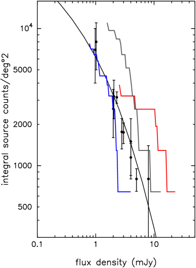
Figure 7: Histograms representing the 850$\mu$m source-counts from three different small area surveys ($\sim 6$ arcmin²) as shown by the small boxes in Figure 2. These are similar in area and depth to SCUBA 850$\mu$m survey of the HDF (see Figure 8). The solid-line and data are the same as in Figure 6.

Figure 8: Three deep 850$\mu$m surveys extracted from the simulation in Figure 2 with same area and depth as the SCUBA 850$\mu$m survey of the HDF (shown as a circle inside a black square for comparison).

4 Conclusions and Future Work

We have presented simulated surveys which are made as realistic as possible in order to address some key issues confronting existing and forthcoming millimetre and submillimetre surveys. These simulations assume a model for the luminosity and clustering evolution which is poorly constrained by current data. Improving our understanding of this evolution provides the motivation for conducting submillimetre and millimetre surveys. It is therefore important that we quantify the limitations of these surveys and the significance of the results drawn from them.

In this paper we discuss the results from survey simulations with a range of wavelengths (200$\mu$m – 1.1 mm), spatial resolutions (6– 27) and flux densities (0.01–310 mJy). Several issues have been addressed related to the estimation of the measured source-counts in future surveys: resolution and confusion; survey sensitivity and noise; and sampling variance due to clustering and shot-noise.

The redshift information, determined from the millimetre and submillimetre colours of individual sources (Hughes 2000), is an essential ingredient to discriminate between the possible evolutionary models that describe the star formation history of galaxies.

Clustering in future wide-area submillimetre surveys might also help to understand some of these issues. Both the number counts and the two-point clustering pattern depend strongly on the cosmological model, but its combination can break some degeneracies. For example if galaxy formation occurs in the rare peaks of the underlying matter field then the resulting galaxy clustering should be stronger than if galaxy formation occurred in random places. The measure of the coherence of the clustering pattern, as described by the higher-order statistics (which is apparent in our simulated maps), can also be used to test how star forming galaxies trace the underlying mass (e.g. Gaztañaga 2000, and references therein). This issues will be address in more detail elsewhere.

References

- [] Barger, A.J. et al. 1998, Nature, 394, 248
- [] Barger, A.J., Cowie, L.L., Sanders, D.B. 1999, ApJ, 518, L5
- [] Dwek, E. et al. 1998, ApJ 508, 106
- [] Eales, S.A. et al. 1999, ApJ, 515, 518
- [] Gaztañaga, E. & Baugh, C. 1998, MNRAS, 294, 229
- [] Gaztañaga, E., 1995, ApJ, 454, 561
- [] Gaztañaga, E., 2000, astro-h/0003160
- [] Giavalisco, M. et al. 1998, ApJ, 503, 543
- [] Hughes, D.H. & Gaztañaga, E., 2000, MNRAS, in preparation
- [] Hughes, D.H. et al. 1998, Nature, 394, 241
- [] Hughes, D.H., 2000, astro-ph/0003414
- [] Lilly, S. et al. 1999, ApJ, 518, 441
- [] Saunders, W. et al. 1990, MNRAS, 242, 318
- [] Smail, I. et al. 1997, MNRAS, 490, L5